Appendix E
Time Value of Money
APPENDIX PREVIEW
Would you rather receive NT$1,000 today or a year from now? You should prefer to receive the NT$1,000 today because you can invest the NT$1,000 and earn interest on it. As a result, you will have more than NT$1,000 a year from now. What this example illustrates is the concept of the time value of money. Everyone prefers to receive money today rather than in the future because of the interest factor.
Nature of Interest
Interest Payment for the use of another person's money. It is payment for the use of another person's money. It is the difference between the amount borrowed or invested (called the principal) and the amount repaid or collected. The amount of interest to be paid or collected is usually stated as a rate over a specific period of time. The rate of interest is generally stated as an annual rate.
The amount of interest involved in any financing transaction is based on three elements:
Principal (p): The original amount borrowed or invested.
Interest Rate (i): An annual percentage of the principal.
Time (n): The number of periods that the principal is borrowed or invested.
Simple Interest
Simple interest is computed on the principal only. It is the return on the principal for one period. Simple interest is usually expressed as shown in Illustration E-1.
Illustration E-1 Interest computation
Compound Interest
Compound interest is computed on principal and on any interest earned that has not been paid or withdrawn. It is the return on (or growth of) the principal for two or more time periods. Compounding computes interest not only on the principal but also on the interest earned to date on that principal, assuming the interest is left on deposit.
To illustrate the difference between simple and compound interest, assume that you deposit €1,000 in Bank Two, where it will earn simple interest of 9% per year, and you deposit another €1,000 in Citizens Bank, where it will earn compound interest of 9% per year compounded annually. Also assume that in both cases you will not withdraw any cash until three years from the date of deposit. Illustration E-2 shows the computation of interest to be received and the accumulated year-end balances.
Illustration E-2 Simple versus compound interest
Note in Illustration E-2 that simple interest uses the initial principal of €1,000 to compute the interest in all three years. Compound interest uses the accumulated balance (principal plus interest to date) at each year-end to compute interest in the succeeding year—which explains why your compound interest account is larger.
Obviously, if you had a choice between investing your money at simple interest or at compound interest, you would choose compound interest, all other things—especially risk—being equal. In the example, compounding provides €25.03 of additional interest income. For practical purposes, compounding assumes that unpaid interest earned becomes a part of the principal, and the accumulated balance at the end of each year becomes the new principal on which interest is earned during the next year.
Illustration E-2 indicates that you should invest your money at the bank that compounds interest. Most business situations use compound interest. Simple interest is generally applicable only to short-term situations of one year or less.
Future Value Concepts
Future Value of a Single Amount
The future value of a single amount is the value at a future date of a given amount invested, assuming compound interest. For example, in Illustration E-2, €1,295.03 is the future value of the €1,000 investment earning 9% for three years. The €1,295.03 is determined more easily by using the following formula.

Illustration E-3 Formula for future value
where:
- FV = future value of a single amount
- p = principal (or present value; the value today)
- i = interest rate for one period
- n = number of periods
The €1,295.03 is computed as follows.
The 1.29503 is computed by multiplying (1.09 × 1.09 × 1.09). The amounts in this example can be depicted in the time diagram shown in Illustration E-4.
Illustration E-4 Time diagram
Another method used to compute the future value of a single amount involves a compound interest table. This table shows the future value of 1 for periods. Table 1 (page E‐4) is such a table.
In Table 1, is the number of compounding periods, the percentages are the periodic interest rates, and the 5‐digit decimal numbers in the respective columns are the future value of 1 factors. To use Table 1, you multiply the principal amount by the future value factor for the specified number of periods and interest rate. For example, the future value factor for two periods at 9% is 1.18810. Multiplying this factor by €1,000 equals €1,188.10—which is the accumulated balance at the end of year 2 in the Citizens Bank example in Illustration E-2. The €1,295.03 accumulated balance at the end of the third year is calculated from Table 1 by multiplying the future value factor for three periods (1.29503) by the €1,000.
Table 1 Future Value of 1
| (n) Periods | 4% | 5% | 6% | 7% | 8% | 9% | 10% | 11% | 12% | 15% |
| 0 | 1.00000 | 1.00000 | 1.00000 | 1.00000 | 1.00000 | 1.00000 | 1.00000 | 1.00000 | 1.00000 | 1.00000 |
| 1 | 1.04000 | 1.05000 | 1.06000 | 1.07000 | 1.08000 | 1.09000 | 1.10000 | 1.11000 | 1.12000 | 1.15000 |
| 2 | 1.08160 | 1.10250 | 1.12360 | 1.14490 | 1.16640 | 1.18810 | 1.21000 | 1.23210 | 1.25440 | 1.32250 |
| 3 | 1.12486 | 1.15763 | 1.19102 | 1.22504 | 1.25971 | 1.29503 | 1.33100 | 1.36763 | 1.40493 | 1.52088 |
| 4 | 1.16986 | 1.21551 | 1.26248 | 1.31080 | 1.36049 | 1.41158 | 1.46410 | 1.51807 | 1.57352 | 1.74901 |
| 5 | 1.21665 | 1.27628 | 1.33823 | 1.40255 | 1.46933 | 1.53862 | 1.61051 | 1.68506 | 1.76234 | 2.01136 |
| 6 | 1.26532 | 1.34010 | 1.41852 | 1.50073 | 1.58687 | 1.67710 | 1.77156 | 1.87041 | 1.97382 | 2.31306 |
| 7 | 1.31593 | 1.40710 | 1.50363 | 1.60578 | 1.71382 | 1.82804 | 1.94872 | 2.07616 | 2.21068 | 2.66002 |
| 8 | 1.36857 | 1.47746 | 1.59385 | 1.71819 | 1.85093 | 1.99256 | 2.14359 | 2.30454 | 2.47596 | 3.05902 |
| 9 | 1.42331 | 1.55133 | 1.68948 | 1.83846 | 1.99900 | 2.17189 | 2.35795 | 2.55803 | 2.77308 | 3.51788 |
| 10 | 1.48024 | 1.62889 | 1.79085 | 1.96715 | 2.15892 | 2.36736 | 2.59374 | 2.83942 | 3.10585 | 4.04556 |
| 11 | 1.53945 | 1.71034 | 1.89830 | 2.10485 | 2.33164 | 2.58043 | 2.85312 | 3.15176 | 3.47855 | 4.65239 |
| 12 | 1.60103 | 1.79586 | 2.01220 | 2.25219 | 2.51817 | 2.81267 | 3.13843 | 3.49845 | 3.89598 | 5.35025 |
| 13 | 1.66507 | 1.88565 | 2.13293 | 2.40985 | 2.71962 | 3.06581 | 3.45227 | 3.88328 | 4.36349 | 6.15279 |
| 14 | 1.73168 | 1.97993 | 2.26090 | 2.57853 | 2.93719 | 3.34173 | 3.79750 | 4.31044 | 4.88711 | 7.07571 |
| 15 | 1.80094 | 2.07893 | 2.39656 | 2.75903 | 3.17217 | 3.64248 | 4.17725 | 4.78459 | 5.47357 | 8.13706 |
| 16 | 1.87298 | 2.18287 | 2.54035 | 2.95216 | 3.42594 | 3.97031 | 4.59497 | 5.31089 | 6.13039 | 9.35762 |
| 17 | 1.94790 | 2.29202 | 2.69277 | 3.15882 | 3.70002 | 4.32763 | 5.05447 | 5.89509 | 6.86604 | 10.76126 |
| 18 | 2.02582 | 2.40662 | 2.85434 | 3.37993 | 3.99602 | 4.71712 | 5.55992 | 6.54355 | 7.68997 | 12.37545 |
| 19 | 2.10685 | 2.52695 | 3.02560 | 3.61653 | 4.31570 | 5.14166 | 6.11591 | 7.26334 | 8.61276 | 14.23177 |
| 20 | 2.19112 | 2.65330 | 3.20714 | 3.86968 | 4.66096 | 5.60441 | 6.72750 | 8.06231 | 9.64629 | 16.36654 |
The demonstration problem in Illustration E-5 shows how to use Table 1.
Illustration E-5 Demonstration problem—Using Table 1 for FV of 1
Future Value of an Annuity
The preceding discussion involved the accumulation of only a single principal sum. Individuals and businesses frequently encounter situations in which a series of equal amounts are to be paid or received at evenly spaced time intervals (periodically), such as loans or lease (rental) contracts. A series of payments or receipts of equal amounts is referred to as an annuity.
The future value of an annuity is the sum of all the payments (receipts) plus the accumulated compound interest on them. In computing the future value of an annuity, it is necessary to know (1) the interest rate, (2) the number of payments (receipts), and (3) the amount of the periodic payments (receipts).
To illustrate the computation of the future value of an annuity, assume that you invest HK$2,000 at the end of each year for three years at 5% interest compounded annually. This situation is depicted in the time diagram in Illustration E-6.

Illustration E-6 Time diagram for a three-year annuity
The HK$2,000 invested at the end of year 1 will earn interest for two years (years 2 and 3), and the HK$2,000 invested at the end of year 2 will earn interest for one year (year 3). However, the last HK$2,000 investment (made at the end of year 3) will not earn any interest. Using the future value factors from Table 1, the future value of these periodic payments is computed as shown in Illustration E-7.

Illustration E-7 Future value of periodic payment computation
The first HK$2,000 investment is multiplied by the future value factor for two periods (1.1025) because two years' interest will accumulate on it (in years 2 and 3). The second HK$2,000 investment will earn only one year's interest (in year 3) and therefore is multiplied by the future value factor for one year (1.0500). The final HK$2,000 investment is made at the end of the third year and will not earn any interest. Thus, and the future value factor is 1.00000. Consequently, the future value of the last HK$2,000 invested is only HK$2,000 since it does not accumulate any interest.
Calculating the future value of each individual cash flow is required when the periodic payments or receipts are not equal in each period. However, when the periodic payments (receipts) are the same in each period, the future value can be computed by using a future value of an annuity of 1 table. Table 2 (page E-6) is such a table.
TABLE 2 Future Value of an Annuity of 1
| (n) Payments | 4% | 5% | 6% | 7% | 8% | 9% | 10% | 11% | 12% | 15% |
| 1 | 1.00000 | 1.00000 | 1.00000 | 1.0000 | 1.00000 | 1.00000 | 1.00000 | 1.00000 | 1.00000 | 1.00000 |
| 2 | 2.04000 | 2.05000 | 2.06000 | 2.0700 | 2.08000 | 2.09000 | 2.10000 | 2.11000 | 2.12000 | 2.15000 |
| 3 | 3.12160 | 3.15250 | 3.18360 | 3.2149 | 3.24640 | 3.27810 | 3.31000 | 3.34210 | 3.37440 | 3.47250 |
| 4 | 4.24646 | 4.31013 | 4.37462 | 4.4399 | 4.50611 | 4.57313 | 4.64100 | 4.70973 | 4.77933 | 4.99338 |
| 5 | 5.41632 | 5.52563 | 5.63709 | 5.7507 | 5.86660 | 5.98471 | 6.10510 | 6.22780 | 6.35285 | 6.74238 |
| 6 | 6.63298 | 6.80191 | 6.97532 | 7.1533 | 7.33592 | 7.52334 | 7.71561 | 7.91286 | 8.11519 | 8.75374 |
| 7 | 7.89829 | 8.14201 | 8.39384 | 8.6540 | 8.92280 | 9.20044 | 9.48717 | 9.78327 | 10.08901 | 11.06680 |
| 8 | 9.21423 | 9.54911 | 9.89747 | 10.2598 | 10.63663 | 11.02847 | 11.43589 | 11.85943 | 12.29969 | 13.72682 |
| 9 | 10.58280 | 11.02656 | 11.49132 | 11.9780 | 12.48756 | 13.02104 | 13.57948 | 14.16397 | 14.77566 | 16.78584 |
| 10 | 12.00611 | 12.57789 | 13.18079 | 13.8164 | 14.48656 | 15.19293 | 15.93743 | 16.72201 | 17.54874 | 20.30372 |
| 11 | 13.48635 | 14.20679 | 14.97164 | 15.7836 | 16.64549 | 17.56029 | 18.53117 | 19.56143 | 20.65458 | 24.34928 |
| 12 | 15.02581 | 15.91713 | 16.86994 | 17.8885 | 18.97713 | 20.14072 | 21.38428 | 22.71319 | 24.13313 | 29.00167 |
| 13 | 16.62684 | 17.71298 | 18.88214 | 20.1406 | 21.49530 | 22.95339 | 24.52271 | 26.21164 | 28.02911 | 34.35192 |
| 14 | 18.29191 | 19.59863 | 21.01507 | 22.5505 | 24.21492 | 26.01919 | 27.97498 | 30.09492 | 32.39260 | 40.50471 |
| 15 | 20.02359 | 21.57856 | 23.27597 | 25.1290 | 27.15211 | 29.36092 | 31.77248 | 34.40536 | 37.27972 | 47.58041 |
| 16 | 21.82453 | 23.65749 | 25.67253 | 27.8881 | 30.32428 | 33.00340 | 35.94973 | 39.18995 | 42.75328 | 55.71747 |
| 17 | 23.69751 | 25.84037 | 28.21288 | 30.8402 | 33.75023 | 36.97351 | 40.54470 | 44.50084 | 48.88367 | 65.07509 |
| 18 | 25.64541 | 28.13238 | 30.90565 | 33.9990 | 37.45024 | 41.30134 | 45.59917 | 50.39593 | 55.74972 | 75.83636 |
| 19 | 27.67123 | 30.53900 | 33.75999 | 37.3790 | 41.44626 | 46.01846 | 51.15909 | 56.93949 | 63.43968 | 88.21181 |
| 20 | 29.77808 | 33.06595 | 36.78559 | 40.9955 | 45.76196 | 51.16012 | 57.27500 | 64.20283 | 72.05244 | 102.44358 |
Table 2 shows the future value of 1 to be received periodically for a given number of payments. It assumes that each payment is made at the end of each period. We can see from Table 2 that the future value of an annuity of 1 factor for three payments at 5% is 3.15250. The future value factor is the total of the three individual future value factors as shown in Illustration E-7. Multiplying this amount by the annual investment of HK$2,000 produces a future value of HK$6,305.
The demonstration problem in Illustration E-8 shows how to use Table 2.

Illustration E-8 Demonstration problem— Using Table 2 for FV of an annuity of 1
Present Value Concepts
Present Value Variables
The present value is the value now of a given amount to be paid or received in the future, assuming compound interest. The present value, like the future value, is based on three variables: (1) the dollar amount to be received (future amount), (2) the length of time until the amount is received (number of periods), and (3) the interest rate (the discount rate). The process of determining the present value is referred to as discounting the future amount.
Present value computations are used in measuring many items. For example, the present value of principal and interest payments is used to determine the market price of a bond. Determining the amount to be reported for notes payable and lease liabilities also involves present value computations. In addition, capital budgeting and other investment proposals are evaluated using present value computations. Finally, all rate of return and internal rate of return computations involve present value techniques.
Present Value of a Single Amount
To illustrate present value, assume that you want to invest a sum of money today that will provide €1,000 at the end of one year. What amount would you need to invest today to have €1,000 one year from now? If you want a 10% rate of return, the investment or present value is . The formula for calculating present value is shown in Illustration E-9.

Illustration E-9 Formula for present value
The computation of €1,000 discounted at 10% for one year is as follows.
The future amount (€1,000), the discount rate (10%), and the number of periods (1) are known. The variables in this situation can be depicted in the time diagram in Illustration E-10.
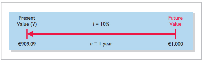
Illustration E-10 Finding present value if discounted for one period
If the single amount of €1,000 is to be received in two years and discounted at , its present value is , depicted in Illustration E-11.

Illustration E-11 Finding present value if discounted for two periods
The present value of 1 may also be determined through tables that show the present value of 1 for periods. In Table 3 below, is the number of discounting periods involved. The percentages are the periodic interest rates or discount rates, and the 5-digit decimal numbers in the respective columns are the present value of 1 factors.
TABLE 3 Present Value of 1
| (n)Periods | 4% | 5% | 6% | 7% | 8% | 9% | 10% | 11% | 12% | 15% |
| 1 | .96154 | .95238 | .94340 | .93458 | .92593 | .91743 | .90909 | .90090 | .89286 | .86957 |
| 2 | .92456 | .90703 | .89000 | .87344 | .85734 | .84168 | .82645 | .81162 | .79719 | .75614 |
| 3 | .88900 | .86384 | .83962 | .81630 | .79383 | .77218 | .75132 | .73119 | .71178 | .65752 |
| 4 | .85480 | .82270 | .79209 | .76290 | .73503 | .70843 | .68301 | .65873 | .63552 | .57175 |
| 5 | .82193 | .78353 | .74726 | .71299 | .68058 | .64993 | .62092 | .59345 | .56743 | .49718 |
| 6 | .79031 | .74622 | .70496 | .66634 | .63017 | .59627 | .56447 | .53464 | .50663 | .43233 |
| 7 | .75992 | .71068 | .66506 | .62275 | .58349 | .54703 | .51316 | .48166 | .45235 | .37594 |
| 8 | .73069 | .67684 | .62741 | .58201 | .54027 | .50187 | .46651 | .43393 | .40388 | .32690 |
| 9 | .70259 | .64461 | .59190 | .54393 | .50025 | .46043 | .42410 | .39092 | .36061 | .28426 |
| 10 | .67556 | .61391 | .55839 | .50835 | .46319 | .42241 | .38554 | .35218 | .32197 | .24719 |
| 11 | .64958 | .58468 | .52679 | .47509 | .42888 | .38753 | .35049 | .31728 | .28748 | .21494 |
| 12 | .62460 | .55684 | .49697 | .44401 | .39711 | .35554 | .31863 | .28584 | .25668 | .18691 |
| 13 | .60057 | .53032 | .46884 | .41496 | .36770 | .32618 | .28966 | .25751 | .22917 | .16253 |
| 14 | .57748 | .50507 | .44230 | .38782 | .34046 | .29925 | .26333 | .23199 | .20462 | .14133 |
| 15 | .55526 | .48102 | .41727 | .36245 | .31524 | .27454 | .23939 | .20900 | .18270 | .12289 |
| 16 | .53391 | .45811 | .39365 | .33873 | .29189 | .25187 | .21763 | .18829 | .16312 | .10687 |
| 17 | .51337 | .43630 | .37136 | .31657 | .27027 | .23107 | .19785 | .16963 | .14564 | .09293 |
| 18 | .49363 | .41552 | .35034 | .29586 | .25025 | .21199 | .17986 | .15282 | .13004 | .08081 |
| 19 | .47464 | .39573 | .33051 | .27615 | .23171 | .19449 | .16351 | .13768 | .11611 | .07027 |
| 20 | .45639 | .37689 | .31180 | .25842 | .21455 | .17843 | .14864 | .12403 | .10367 | .06110 |
When using Table 3, the future value is multiplied by the present value factor specified at the intersection of the number of periods and the discount rate. For example, the present value factor for one period at a discount rate of 10% is .90909, which equals the computed in Illustration E-10. For two periods at a discount rate of 10%, the present value factor is .82645, which equals the computed previously.
Note that a higher discount rate produces a smaller present value. For example, using a 15% discount rate, the present value of €1,000 due one year from now is €869.57, versus €909.09 at 10%. Also note that the further removed from the present the future value is, the smaller the present value. For example, using the same discount rate of 10%, the present value of €1,000 due in five years is €620.92. The present value of €1,000 due in one year is €909.09, a difference of €288.17.
The following two demonstration problems (Illustrations 12 and 13) illustrate how to use Table 3.

Illustration E-12 Demonstration problem—Using Table 3 for PV of 1

Illustration E-13 Demonstration problem—Using Table 3 for PV of 1
Present Value of an Annuity
The preceding discussion involved the discounting of only a single future amount. Businesses and individuals frequently engage in transactions in which a series of equal amounts are to be received or paid at evenly spaced time intervals (periodically). Examples of a series of periodic receipts or payments are loan agreements, installment sales, mortgage notes, lease (rental) contracts, and pension obligations. As discussed earlier, these periodic receipts or payments are annuities.
The present value of an annuity is the value now of a series of future receipts or payments, discounted assuming compound interest. In computing the present value of an annuity, it is necessary to know (1) the discount rate, (2) the number of payments (receipts), and (3) the amount of the periodic payments or receipts. To illustrate the computation of the present value of an annuity, assume that you will receive €1,000 cash annually for three years at a time when the discount rate is 10%. This situation is depicted in the time diagram in Illustration E-14. Illustration E-15 shows the computation of its present value in this situation.

Illustration E-14 Time diagram for a three-year annuity

Illustration E-15 Present value of a series of future amounts computation
This method of calculation is required when the periodic cash flows are not uniform in each period. However, when the future receipts are the same in each period, an annuity table can be used. As illustrated in Table 4 below, an annuity table shows the present value of 1 to be received periodically for a given number of payments. It assumes that each payment is made at the end of each period.
TABLE 4 Present Value of an Annuity of 1
| (n) Payments | 4% | 5% | 6% | 7% | 8% | 9% | 10% | 11% | 12% | 15% |
| 1 | .96154 | .95238 | .94340 | .93458 | .92593 | .91743 | .90909 | .90090 | .89286 | .86957 |
| 2 | 1.88609 | 1.85941 | 1.83339 | 1.80802 | 1.78326 | 1.75911 | 1.73554 | 1.71252 | 1.69005 | 1.62571 |
| 3 | 2.77509 | 2.72325 | 2.67301 | 2.62432 | 2.57710 | 2.53130 | 2.48685 | 2.44371 | 2.40183 | 2.28323 |
| 4 | 3.62990 | 3.54595 | 3.46511 | 3.38721 | 3.31213 | 3.23972 | 3.16986 | 3.10245 | 3.03735 | 2.85498 |
| 5 | 4.45182 | 4.32948 | 4.21236 | 4.10020 | 3.99271 | 3.88965 | 3.79079 | 3.69590 | 3.60478 | 3.35216 |
| 6 | 5.24214 | 5.07569 | 4.91732 | 4.76654 | 4.62288 | 4.48592 | 4.35526 | 4.23054 | 4.11141 | 3.78448 |
| 7 | 6.00205 | 5.78637 | 5.58238 | 5.38929 | 5.20637 | 5.03295 | 4.86842 | 4.71220 | 4.56376 | 4.16042 |
| 8 | 6.73274 | 6.46321 | 6.20979 | 5.97130 | 5.74664 | 5.53482 | 5.33493 | 5.14612 | 4.96764 | 4.48732 |
| 9 | 7.43533 | 7.10782 | 6.80169 | 6.51523 | 6.24689 | 5.99525 | 5.75902 | 5.53705 | 5.32825 | 4.77158 |
| 10 | 8.11090 | 7.72173 | 7.36009 | 7.02358 | 6.71008 | 6.41766 | 6.14457 | 5.88923 | 5.65022 | 5.01877 |
| 11 | 8.76048 | 8.30641 | 7.88687 | 7.49867 | 7.13896 | 6.80519 | 6.49506 | 6.20652 | 5.93770 | 5.23371 |
| 12 | 9.38507 | 8.86325 | 8.38384 | 7.94269 | 7.53608 | 7.16073 | 6.81369 | 6.49236 | 6.19437 | 5.42062 |
| 13 | 9.98565 | 9.39357 | 8.85268 | 8.35765 | 7.90378 | 7.48690 | 7.10336 | 6.74987 | 6.42355 | 5.58315 |
| 14 | 10.56312 | 9.89864 | 9.29498 | 8.74547 | 8.24424 | 7.78615 | 7.36669 | 6.98187 | 6.62817 | 5.72448 |
| 15 | 11.11839 | 10.37966 | 9.71225 | 9.10791 | 8.55948 | 8.06069 | 7.60608 | 7.19087 | 6.81086 | 5.84737 |
| 16 | 11.65230 | 10.83777 | 10.10590 | 9.44665 | 8.85137 | 8.31256 | 7.82371 | 7.37916 | 6.97399 | 5.95424 |
| 17 | 12.16567 | 11.27407 | 10.47726 | 9.76322 | 9.12164 | 8.54363 | 8.02155 | 7.54879 | 7.11963 | 6.04716 |
| 18 | 12.65930 | 11.68959 | 10.82760 | 10.05909 | 9.37189 | 8.75563 | 8.20141 | 7.70162 | 7.24967 | 6.12797 |
| 19 | 13.13394 | 12.08532 | 11.15812 | 10.33560 | 9.60360 | 8.95012 | 8.36492 | 7.83929 | 7.36578 | 6.19823 |
| 20 | 13.59033 | 12.46221 | 11.46992 | 10.59401 | 9.81815 | 9.12855 | 8.51356 | 7.96333 | 7.46944 | 6.25933 |
Table 4 shows that the present value of an annuity of 1 factor for three payments at 10% is 2.48685.1 This present value factor is the total of the three individual present value factors, as shown in Illustration E-15. Applying this amount to the annual cash flow of €1,000 produces a present value of €2,486.85.
The following demonstration problem (Illustration E-16) illustrates how to use Table 4.
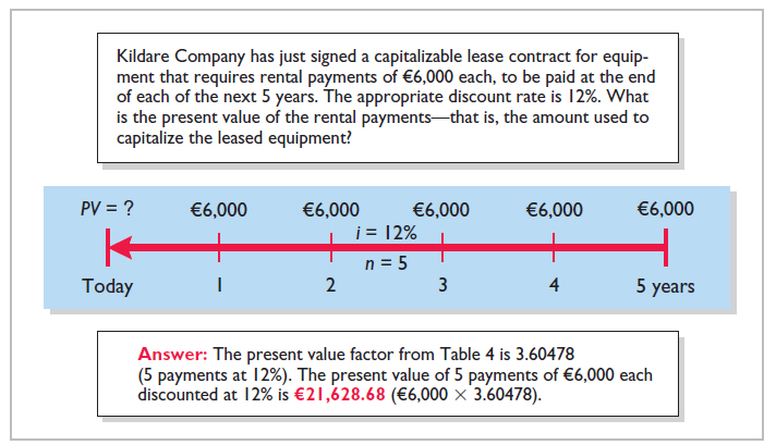
Illustration E-16 Demonstration problem—Using Table 4 for PV of an annuity of 1
Time Periods and Discounting
In the preceding calculations, the discounting was done on an annual basis using an annual interest rate. Discounting may also be done over shorter periods of time such as monthly, quarterly, or semiannually.
When the time frame is less than one year, it is necessary to convert the annual interest rate to the applicable time frame. Assume, for example, that the investor in Illustration E-14 received €500 semiannually for three years instead of €1,000 annually. In this case, the number of periods becomes six , the discount rate is , the present value factor from Table 4 is 5.07569 (6 periods at 5%), and the present value of the future cash flows is . This amount is slightly higher than the €2,486.86 computed in Illustration E-15 because interest is computed twice during the same year. That is, during the second half of the year, interest is earned on the first half-year's interest.
Computing the Present Value of a Long-Term Note or Bond
The present value (or market price) of a long-term note or bond is a function of three variables: (1) the payment amounts, (2) the length of time until the amounts are paid, and (3) the discount rate. Our example uses a five-year bond issue.
The first variable (amounts to be paid) is made up of two elements: (1) a series of interest payments (an annuity) and (2) the principal amount (a single sum). To compute the present value of the bond, both the interest payments and the principal amount must be discounted—;two different computations. The time diagrams for a bond due in five years are shown in Illustration E-17.

Illustration E-17 Present value of a bond time diagram
When the investor's market interest rate is equal to the bond's contractual interest rate, the present value of the bonds will equal the face value of the bonds. To illustrate, assume a bond issue of 10%, five-year bonds with a face value of NT$100,000 with interest payable semiannually on January 1 and July 1. If the discount rate is the same as the contractual rate, the bonds will sell at face value. In this case, the investor will receive (1) NT$100,000 at maturity and (2) a series of ten NT$5,000 interest payments over the term of the bonds. The length of time is expressed in terms of interest periods—in this case—10, and the discount rate per interest period, 5%. The following time diagram (Illustration E-18) depicts the variables involved in this discounting situation.

Illustration E-18 Time diagram for present value of a 10%, five-year bond paying interest semiannually
Illustration E-19 shows the computation of the present value of these bonds.

Illustration E-19 Present value of principal and interest—face value
Now assume that the investor's required rate of return is 12%, not 10%. The future amounts are again NT$100,000 and NT$5,000, respectively, but now a discount rate of must be used. The present value of the bonds is NT$92,639, as computed in Illustration E-20.
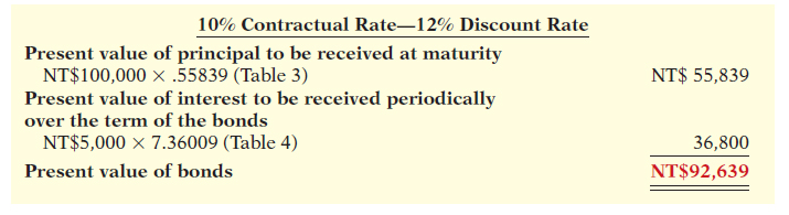
Illustration E-20 Present value of principal and interest—discount
Conversely, if the discount rate is 8% and the contractual rate is 10%, the present value of the bonds is NT$108,111, computed as shown in Illustration E-21.

Illustration E-21 Present value of principal and interest—premium
The above discussion relied on present value tables in solving present value problems. Calculators may also be used to compute present values without the use of these tables. Many calculators, especially financial calculators, have present value (PV) functions that allow you to calculate present values by merely inputting the proper amount, discount rate, periods, and pressing the PV key. We discuss the use of financial calculators in a later section.
Computing the Present Values in a Capital Budgeting Decision
The decision to make long-term capital investments is best evaluated using discounting techniques that recognize the time value of money. To do this, many companies calculate the present value of the cash flows involved in a capital investment.
To illustrate, Nagel-Siebert Trucking Company, a cross-country freight carrier, is considering adding another truck to its fleet because of a purchasing opportunity. Nagel-Siebert's primary supplier of overland rigs is overstocked and offers to sell its biggest rig for £154,000 cash payable upon delivery. Nagel-Siebert knows that the rig will produce a net cash flow per year of £40,000 for five years (received at the end of each year), at which time it will be sold for an estimated residual value of £35,000. Nagel-Siebert's discount rate in evaluating capital expenditures is 10%. Should Nagel-Siebert commit to the purchase of this rig?
The cash flows that must be discounted to present value by Nagel-Siebert are as follows.
Cash payable on delivery (today): £154,000.
Net cash flow from operating the rig: £40,000 for 5 years (at the end of each year).
Cash received from sale of rig at the end of 5 years: £35,000.
The time diagrams for the latter two cash flows are shown in Illustration E-22.
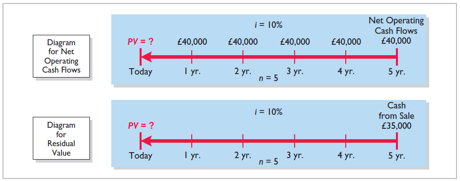
Illustration E-22 Time diagrams for Nagel-Siebert Trucking Company
Notice from the diagrams that computing the present value of the net operating cash flows (£40,000 at the end of each year) is discounting an annuity (Table 4), while computing the present value of the £35,000 residual value is discounting a single sum (Table 3). The computation of these present values is shown in Illustration E-23 (page E-15).

Illustration E-23 Present value computations at 10%
Because the present value of the cash receipts (inflows) of exceeds the present value of the cash payments (outflows) of £154,000.00, the net present value of £19,363.80 is positive, and the decision to invest should be accepted.
Now assume that Nagel-Siebert uses a discount rate of 15%, not 10%, because it wants a greater return on its investments in capital assets. The cash receipts and cash payments by Nagel-Siebert are the same. The present values of these receipts and cash payments discounted at 15% are shown in Illustration E-14.

Illustration E-24 Present value computations at 15%
Because the present value of the cash payments (outflows) of £154,000.00 exceeds the present value of the cash receipts (inflows) of , the net present value of £2,512.30 is negative, and the investment should be rejected.
The above discussion relied on present value tables in solving present value problems. As we show in the next section, calculators may also be used to compute present values without the use of these tables. Some calculators, especially the “business” or financial calculators, have present value (PV) functions that allow you to calculate present values by merely identifying the proper amount, discount rate, periods, and pressing the PV key.
Using Financial Calculators
Business professionals, once they have mastered the underlying time value of money concepts, often use a financial calculator to solve these types of problems. In most cases, they use calculators if interest rates or time periods do not correspond with the information provided in the compound interest tables.
To use financial calculators, you enter the time value of money variables into the calculator. Illustration E-25 shows the five most common keys used to solve time value of money problems.2

Illustration E-25 Financial calculator keys
where:
In solving time value of money problems in this appendix, you will generally be given three of four variables and will have to solve for the remaining variable. The fifth key (the key not used) is given a value of zero to ensure that this variable is not used in the computation.
Present Value of a Single Sum
To illustrate how to solve a present value problem using a financial calculator, assume that you want to know the present value of €84,253 to be received in five years, discounted at 11% compounded annually. Illustration E-26 depicts this problem.

Illustration E-26 Calculator solution for present value of a single sum
Illustration E-26 shows you the information (inputs) to enter into the calculator: , , , and . You then press PV for the answer: . As indicated, the PMT key was given a value of zero because a series of payments did not occur in this problem.
PLUS AND MINUS
The use of plus and minus signs in time value of money problems with a financial calculator can be confusing. Most financial calculators are programmed so that the positive and negative cash flows in any problem offset each other. In the present value problem above, we identified the €84,253 future value initial investment as a positive (inflow); the answer was shown as a negative amount, reflecting a cash outflow. If the 84,253 were entered as a negative, then the final answer would have been reported as a positive 50,000.
Hopefully, the sign convention will not cause confusion. If you understand what is required in a problem, you should be able to interpret a positive or negative amount in determining the solution to a problem.
COMPOUNDING PERIODS
In the previous problem, we assumed that compounding occurs once a year. Some financial calculators have a default setting, which assumes that compounding occurs 12 times a year. You must determine what default period has been programmed into your calculator and change it as necessary to arrive at the proper compounding period.
ROUNDING
Most financial calculators store and calculate using 12 decimal places. As a result, because compound interest tables generally have factors only up to five decimal places, a slight difference in the final answer can result. In most time value of money problems, the final answer will not include more than two decimal places.
Present Value of an Annuity
To illustrate how to solve a present value of an annuity problem using a financial calculator, assume that you are asked to determine the present value of rental receipts of €6,000 each to be received at the end of each of the next five years, when discounted at 12%, as pictured in Illustration E-27.

Illustration E-27 Calculator solution for present value of an annuity
In this case, you enter , , , , , and then press PV to arrive at the answer of .
Useful Applications of the Financial Calculator
With a financial calculator, you can solve for any interest rate or for any number of periods in a time value of money problem. Here are some examples of these applications.
AUTO LOAN
Assume you are financing the purchase of a used car with a three-year loan. The loan has a 9.5% stated annual interest rate, compounded monthly. The price of the car is €6,000, and you want to determine the monthly payments, assuming that the payments start one month after the purchase. This problem is pictured in Illustration E-28.

Illustration E-28 Calculator solution for auto loan payments
To solve this problem, you enter , , , , and than press PMT. You will find that the monthly payments will be €192.20. Note that the payment key is usually programmed for 12 payments per year. Thus, you must change the default (compounding period) if the payments are other than monthly.
MORTGAGE LOAN AMOUNT
Say you are evaluating financing options for a loan on a house (a mortgage). You decide that the maximum mortgage payment you can afford is €700 per month. The annual interest rate is 8.4%. If you get a mortgage that requires you to make monthly payments over a 15-year period, what is the maximum home loan you can afford? Illustration E-29 depicts this problem.

Illustration E-29 Calculator solution for mortgage amount
You enter , , , , and press PV. With the payments-per-year key set at 12, you find a present value of €71,509.81— the maximum home loan you can afford, given that you want to keep your mortgage payments at €700. Note that by changing any of the variables, you can quickly conduct “what-if” analyses for different situations.
REVIEW
LEARNING OBJECTIVES REVIEW
Distinguish between simple and compound interest. Simple interest is computed on the principal only, while compound interest is computed on the principal and any interest earned that has not been withdrawn.
Solve for future value of a single amount. Prepare a time diagram of the problem. Identify the principal amount, the number of compounding periods, and the interest rate. Using the future value of 1 table, multiply the principal amount by the future value factor specified at the intersection of the number of periods and the interest rate.
Solve for future value of an annuity. Prepare a time diagram of the problem. Identify the amount of the periodic payments (receipts), the number of payments (receipts), and the interest rate. Using the future value of an annuity of 1 table, multiply the amount of the payments by the future value factor specified at the intersection of the number of periods and the interest rate.
Identify the variables fundamental to solving present value problems. The following three variables are fundamental to solving present value problems: (1) the future amount, (2) the number of periods, and (3) the interest rate (the discount rate).
Solve for present value of a single amount. Prepare a time diagram of the problem. Identify the future amount, the number of discounting periods, and the discount (interest) rate. Using the present value of a single amount table, multiply the future amount by the present value factor specified at the intersection of the number of periods and the discount rate.
Solve for present value of an annuity. Prepare a time diagram of the problem. Identify the amount of future periodic receipts or payment (annuities), the number of payments (receipts), and the discount (interest) rate. Using the present value of an annuity of 1 table, multiply the amount of the annuity by the present value factor specified at the intersection of the number of payments and the interest rate.
Compute the present value of notes and bonds. Determine the present value of the principal amount: Multiply the principal amount (a single future amount) by the present value factor (from the present value of 1 table) intersecting at the number of periods (number of interest payments) and the discount rate. Determine the present value of the series of interest payments: Multiply the amount of the interest payment by the present value factor (from the present value of an annuity of 1 table) intersecting at the number of periods (number of interest payments) and the discount rate. Add the present value of the principal amount to the present value of the interest payments to arrive at the present value of the note or bond.
Compute the present values in capital budgeting situations. Compute the present values of all cash inflows and all cash outflows related to the capital budgeting proposal (an investment-type decision). If the net present value is positive, accept the proposal (make the investment). If the net present value is negative, reject the proposal (do not make the investment).
Use a financial calculator to solve time value of money problems. Financial calculators can be used to solve the same and additional problems as those solved with time value of money tables. Enter into the financial calculator the amounts for all of the known elements of a time value of money problem (periods, interest rate, payments, future or present value), and it solves for the unknown element. Particularly useful situations involve interest rates and compounding periods not presented in the tables.
GLOSSARY REVIEW
- Annuity
- A series of equal dollar amounts to be paid or received at evenly spaced time intervals (periodically). (p. E-4).
- Compound interest
- The interest computed on the principal and any interest earned that has not been paid or withdrawn. (p. E-2).
- Discounting the future amount(s)
- The process of determining present value. (p. E-7).
- Future value of an annuity
- The sum of all the payments (receipts) plus the accumulated compound interest on them. (p. E-5).
- Future value of a single amount
- The value at a future date of a given amount invested, assuming compound interest. (p. E-3).
- Interest
- Payment for the use of another person’s money. (p. E-1).
- Present value
- The value now of a given amount to be paid or received in the future assuming compound interest. (p. E-7).
- Present value of an annuity
- The value now of a series of future receipts or payments, discounted assuming compound interest. (p. E-9).
- Principal
- The amount borrowed or invested. (p. E-1).
- Simple interest
- The interest computed on the principal only. (p. E-1).
WileyPLUS
Many more resources are available for practice in WileyPLUS.
BRIEF EXERCISES
(Use tables to solve exercises BEE-1 to BEE-23.)
Compute the future value of a single amount.
BEE-1 Randy Owen invested €9,000 at 5% annual interest, and left the money invested without withdrawing any of the interest for 15 years. At the end of the 15 years, Randy withdrew the accumulated amount of money. (a) What amount did Randy withdraw, assuming the investment earns simple interest? (b) What amount did Randy withdraw, assuming the investment earns interest compounded annually?
Use future value tables.
BEE-2 For each of the following cases, indicate (a) to what interest rate columns and (b) to what number of periods you would refer in looking up the future value factor.
- (1) In Table 1 (future value of 1):
Annual Rate Number of Years Invested Compounded Case A 5% 3 Annually Case B 12% 4 Semiannually - In Table 2 (future value of an annuity of 1):
Annual Rate Number of Years Invested Compounded Case A 3% 8 Annually Case B 8% 6 Semiannually
Compute the future value of a single amount.
BEE-3 Joyce Ltd. signed a lease for an office building for a period of 8 years. Under the lease agreement, a security deposit of £8,400 is made. The deposit will be returned at the expiration of the lease with interest compounded at 4% per year. What amount will Joyce receive at the time the lease expires?
Compute the future value of an annuity.
BEE-4 Bates Company issued $1,000,000, 12-year bonds and agreed to make annual sinking fund deposits of $60,000. The deposits are made at the end of each year into an account paying 6% annual interest. What amount will be in the sinking fund at the end of 12 years?
Compute the future value of a single amount and of an annuity.
BEE-5 Frank and Maureen Fantazzi invested €8,000 in a savings account paying 5% annual interest when their daughter, Angela, was born. They also deposited €1,000 on each of her birthdays until she was 18 (including her 18th birthday). How much was in the savings account on her 18th birthday (after the last deposit)?
Compute the future value of a single amount.
BEE-6 Hugh Curtin borrowed $35,000 on July 1, 2017. This amount plus accrued interest at 8% compounded annually is to be repaid on July 1, 2022. How much will Hugh have to repay on July 1, 2022?
Use present value tables.
BEE-7 For each of the following cases, indicate (a) to what interest rate columns and (b) to what number of periods you would refer in looking up the discount rate.
- In Table 3 (present value of 1):
Annual Rate Number of Years Involved Discounts per Year Case A 12% 7 Semiannually Case B 8% 11 Annually Case C 10% 8 Semiannually - In Table 4 (present value of an annuity of 1):
Annual Rate Number of Years Involved Number of Payments Involved Frequency of Payments Case A 10% 20 20 Annually Case B 10% 7 7 Annually Case C 8% 5 10 Semiannually
Determine present values.
BEG-8 What is the present value of $25,000 due 9 periods from now, discounted at 10%?
What is the present value of $25,000 to be received at the end of each of 6 periods, discounted at 9%?
Compute the present value of a single amount investment.
BEG-9 Pingtung Ltd. is considering an investment that will return a lump sum of NT$750,000 eight years from now. What amount should Pingtung pay for this investment to earn an 5% return?
Compute the present value of a single amount investment.
BEG-10 Lloyd Company earns 6% on an investment that will return $450,000 eight years from now. What is the amount Lloyd should invest now to earn this rate of return?
Compute the present value of an annuity investment.
BEG-11 Arthur plc is considering investing in an annuity contract that will return £46,000 annually at the end of each year for 12 years. What amount should Arthur pay for this investment if it earns an 7% return?
Compute the present value of an annual investment.
BEG-12 Kaehler Enterprises earns 5% on an investment that pays back $80,000 at the end of each of the next 6 years. What is the amount Kaehler invested to earn the 5% rate of return?
Compute the present value of bonds.
BEG-13 Hanna Railroad Co. is about to issue €300,000 of 10-year bonds paying an 11% interest rate, with interest payable semiannually. The discount rate for such securities is 10%. How much can Hanna expect to receive for the sale of these bonds?
Compute the present value of bonds.
BEG-14 Assume the same information as BEE-13 except that the discount rate is 12% instead of 10%. In this case, how much can Hanna expect to receive from the sale of these bonds?
Compute the present value of a note.
BEG-15 Yilan Ltd. receives a NT$48,000, 5-year note bearing interest of 4% (paid annually) from a customer at a time when the discount rate is 6%. What is the present value of the note received by Yilan?
Compute the present value of a note.
BEG-15 Yilan Ltd. receives a NT$48,000, 5-year note bearing interest of 4% (paid annually) from a customer at a time when the discount rate is 6%. What is the present value of the note received by Yilan?
Compute the present value of bonds.
BEG-16 Gleason Enterprises issued 6%, 8-year, $2,500,000 par value bonds that pay interest semiannually on October 1 and April 1. The bonds are dated April 1, 2017, and are issued on that date. The discount rate of interest for such bonds on April 1, 2017, is 8%. What cash proceeds did Gleason receive from issuance of the bonds?
Compute the present value of a machine for purposes of making a purchase decision.
BEG-17 Mark Barton owns a garage and is contemplating purchasing a tire retreading machine for $20,000. After estimating costs and revenues, Mark projects a net cash flow from the retreading machine of $3,200 annually for 8 years. Mark hopes to earn a return of 7% on such investments. What is the present value of the retreading operation? Should Mark purchase the retreading machine?
Compute the present value of a note.
BEG-18 Frazier Company issues a 10%, 5-year mortgage note on January 1, 2017, to obtain financing for new equipment. Land is used as collateral for the note. The terms provide for semiannual installment payments of $48,850. What were the cash proceeds received from the issuance of the note?
Compute the maximum price to pay for a machine.
BEG-19 Wei Ltd. is considering purchasing equipment. The equipment will produce the following cash flows: Year 1, ¥40,000; Year 2, ¥43,000; and Year 3, ¥45,000. Wei requires a minimum rate of return of 8%. What is the maximum price Wei should pay for this equipment?
Compute the interest rate on a single amount.
BEG-20 If Colleen Mooney invests $4,765.50 now and she will receive $12,000 at the end of 12 years, what annual rate of interest will Colleen earn on her investment? (Hint: Use Table 3.)
Compute the number of periods of a single amount.
BEG-21 Wayne Kurt has been offered the opportunity of investing $31,681 now. The investment will earn 9% per year and at the end of that time will return Wayne $75,000. How many years must Wayne wait to receive $75,000? (Hint: Use Table 3.)
Compute the interest rate on an annuity.
BEG-22 Joanne Quick made an investment of $10,271.38. From this investment, she will receive $1,200 annually for the next 15 years starting one year from now. What rate of interest will Joanne's investment be earning for her? (Hint: Use Table 4.)
Compute the number of payments of an annuity.
BEG-23 Patty Schleis invests €6,673.16 now for a series of €1,400 annual returns beginning one year from now. Patty will earn a return of 7% on the initial investment. How many annual payments of €1,400 will Patty receive? (Hint: Use Table 4.)
Determine interest rate.
BEG-24 Carly Simon wishes to invest $18,000 on July 1, 2017, and have it accumulate to $50,000 by July 1, 2027. Use a financial calculator to determine at what exact annual rate of interest Carly must invest the $18,000.
Determine interest rate.
BEG-25 On July 17, 2017, James Taylor borrowed $66,000 from his grandfather to open a clothing store. Starting July 17, 2018, James has to make 8 equal annual payments of $11,225 each to repay the loan. Use a financial calculator to determine what interest rate James is paying.
Determine interest rate.
BEG-26 As the purchaser of a new house, Carrie Underwood has signed a mortgage note to pay the Nashville National Bank and Trust Co. $8,400 every 6 months for 20 years, at the end of which time she will own the house. At the date the mortgage is signed, the purchase price was $198,000 and Underwood made a down payment of $20,000. The first payment will be made 6 months after the date the mortgage is signed. Using a financial calculator, compute the exact rate of interest earned on the mortgage by the bank.
Various time value of money situations.
BEG-27 Using a financial calculator, solve for the unknowns in each of the following situations.
- On June 1, 2016, Holly Golightly purchases lakefront property from her neighbor, George Peppard, and agrees to pay the purchase price in seven payments of $22,000 each, the first payment to be payable June 1, 2017. (Assume that interest compounded at an annual rate of 5.4% is implicit in the payments.) What is the purchase price of the property?
- On January 1, 2016, Sammis Corporation purchased 200 of the $1,000 face value, 7% coupon, 10-year bonds of Malone Inc. The bonds mature on January 1, 2026, and pay interest annually beginning January 1, 2017. Sammis purchased the bonds to yield 8.65%. How much did Sammis pay for the bonds?
Various time value of money situations.
BEG-28 Using a financial calculator, provide a solution to each of the following situations.
- Lynn Anglin owes a debt of $42,000 from the purchase of her new sport utility vehicle. The debt bears annual interest of 7.8% compounded monthly. Lynn wishes to pay the debt and interest in equal monthly payments over 8 years, beginning one month hence. What equal monthly payments will pay off the debt and interest?
- On January 1, 2017, Roger Molony offers to buy Dave Feeney's used snowmobile for $8,000, payable in five equal annual installments, which are to include 7.25% interest on the unpaid balance and a portion of the principal. If the first payment is to be made on December 31, 2017, how much will each payment be?