6.1 INTRODUCTION

With technological advances in multimedia processing and wireless networking, live video content can now be streamed to wireless devices over the Internet. To serve geographically distributed clients,¹ the stream is distributed using a cloud, with the wireless clients independently pulling the stream via an access point (AP) or base station. This model suffers from last‐hop scalability problem—as the number of clients served by the AP increases, its wireless bandwidth becomes a bottleneck (wireless broadcasting standard is not yet widely used nowadays). To overcome such limitation and scale up the last‐hop user capacity, the wireless devices may form a wireless fog, where they collaboratively share the live stream they pulled from the AP with their neighbors in a multihop manner via a secondary channel (such as Bluetooth, Wi‐Fi, etc.). In a wireless fog for live video, devices hence donate their resources (computing power, storage, and communication bandwidth) to scale up the system in a cost‐effective manner.

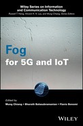
We illustrate in Figure 6.1 a typical live streaming network. The streaming cloud distributes the live stream over the Internet. The cloud is integrated with a wireless fog. In the fog, a source node first pulls the stream from a nearby cloud server through an AP or base station. It then distributes its stream to nearby clients. By cooperatively relaying (rebroadcasting) their received packets, nodes can efficiently distribute the live stream within the fog. In this chapter, “broadcasting” means delivering a packet to all the one‐hop neighbors of the “broadcaster” by sending just one packet (the so‐called broadcast packet).

In a wireless fog, conventionally the live stream is distributed using the “store‐and‐forward” approach, where selected broadcasters simply forward their received packets to their neighbors. As packet loss is inevitable in packet broadcasting, this approach suffers from loss propagation, resulting in high loss toward the leaves of the broadcasting tree. In order to achieve good video playback quality, the loss needs to be mitigated through efficient recovery strategies.

Losses in network transmissions are traditionally recovered by feedback‐based source retransmission. This is not scalable to a large pool of clients due to the bandwidth limitation of the wireless channel and at the source. Random linear network coding (RLNC) lets the video source perform network coding (NC) on every k source packets and broadcast coded packets to clients. This approach requires the knowledge of network loss condition and is often designed for certain worst‐case loss (i.e., ). In diverse loss conditions, RLNC therefore often leads to high redundancy for low‐loss receivers but “starves” high‐loss receivers with insufficient number of packets. In contrast, cooperative loss recovery between neighboring nodes can adapt recovery packets to local loss conditions. One may use source packet sharing, but it limits the recovery efficiency. With the broadcast nature of wireless transmissions, NC can be applied over a selected subset of source packets according to neighbors’ loss status to further improve the efficiency and flexibility of cooperative recovery.

In this chapter, we propose a “store–recover–forward” approach for effective video live streaming over wireless multihop networks. A node repeatedly goes through the following steps:

1. Store: Buffer Some Video Packets for Recovery. A node first buffers received video packets, with the packet availability indicated as a bitmap. As packets may be lost, there may be holes in the bitmap.
2. Recover: Cooperative Recovery Using NC. The node shares its bitmap to its neighbors by broadcasting. It also receives the bitmaps from its neighbors. Based on the received bitmaps, the node selects some of its received packets, applies NC to them, and broadcasts the NC packets to its neighbors. Generating NC packets based on packet subset can lead to more flexible recovery.

   After such broadcasting, the node also receives some NC packets from its neighbors. It uses these NC packets to recover some, if not all, of its lost packets in the bitmap. Neighboring nodes hence work together to selectively and effectively recover their losses.

3. Forward: Video Packets Forwarding. After the aforementioned NC‐based cooperative recovery, the node then exchanges its updated bitmap with neighbors. Based on that, the node decides which packets to forward to its neighbors.

We show in Figure 6.2 an example of wireless live video streaming mesh. Nodes are arranged according to their shortest hop distances to the source. Nodes A, B, and C each first receives some video packets from the Source. B then shares its bitmap with A and C. After receiving its neighbors’ bitmaps, a node generates NC packets for neighbors with the same hop distance from the source and shares these NC packets. Nodes further away from the source, that is, Nodes D and E, can buffer the NC packets for their later use. Among Nodes A, B, and C, broadcasters are then selected for each packet. In this example, B forwards its video packets to Nodes D and E. D and E then perform the same process to cooperatively recover their losses using NC.

In a wireless fog, bandwidth and device energy are scarce resources. Our objective is, therefore, to reduce the total packets broadcasted given a (possibly heterogeneous) target residual loss rate at each node. There are two important decision problems:

• NC Packet Selection (NCPS). In order to maximize error recovery, a node generates NC packets based on selected subsets of its packets. The NCPS problem is hence to determine at each node which video packet set should be used for NC coding and how many NC packets to generate, based on neighbor information, so as to achieve the target residual loss rate at each neighbor, with minimum NC recovery traffic.
• Broadcaster Selection (BS). This problem determines which packet each node should forward, based on updated neighbor information, in order to achieve the target residual loss rate at each node, with minimum video packet forwarding traffic. This is the so‐called broadcaster selection problem.

For high‐quality video distribution in a wireless fog, we therefore address the following issues in this chapter:

• Problem Formulation and Complexity Analysis. We aim at reducing the total network traffic, which includes both NC recovery traffic and video forwarding traffic, with NCPS and BS as the two subproblems. We show that both NCPS and BS problems are NP‐hard.
• Video Broadcasting with Cooperative Recovery (VBCR), Distributed Live Video Distribution with NC‐Based Cooperative Recovery. In a wireless fog, network condition is often highly dynamic and unpredictable. It is hence impossible to deploy a central controller to collect network‐wide information, compute optimal solution, and distribute the solution in a timely manner. We therefore propose an effective distributed algorithm termed VBCR to tackle the problems. Each node in VBCR independently determines the NC packets to code and which video packets to forward, given a certain target residual loss rate at its neighboring nodes. VBCR is fully distributed, with decisions based on only neighbor information and hence is scalable to a large group.
• Simulation Study. We have conducted extensive simulation studies on VBCR. Our results show that VBCR is efficient compared to other schemes in terms of total network traffic generated.

The remainder of the chapter is organized as follows. We introduce the wireless cooperative live streaming network in Section 6.3. We formulate the problems in study and analyze their hardness in Section 6.4. We describe our distributed algorithm VBCR in detail in Section 6.5. We present illustrative simulation results in Section 6.6 and conclude in Section 6.7.

6.2 RELATED WORK

We next briefly review related work. Peer‐cooperative wireless video streaming has been mentioned in many papers [1–4]. There are two main angles: one is to use peers as relays and the other is to use the local neighbors for cooperative loss recovery. The work in Ref. [3] is a typical work of the first class, where the device‐to‐device communication is applied to help improve the received video quality. In both Refs. [1, 2], a source server streams video to users directly, while the packet loss that happened over the primary channel (server‐to‐user channel) are recovered by local neighbors’ help via the secondary channel (user‐to‐user channel) instead of server retransmission. The work in Ref. [4] proposes cooperative video chunk pulling to reduce redundancy and to reduce chunk loss. However link loss is not considered in the work. A video coding scheme for wireless cooperative video broadcasting is proposed in Ref. [5]. Our work does not depend on the coding scheme optimization; instead we try to optimize application level transmissions. In this chapter we study live video distribution in a wireless cooperative fog video streaming, and the approach is a co‐design of the relay node selection and cooperative loss recovery, which distinguishes our work from these schemes.

A large body of research focuses on delay minimization in point‐to‐point transmission [6– 9]. We instead target at bandwidth and energy conservation in broadcast scenario. Schemes in Refs. [10, 11] try to minimize energy cost in an error‐free environment by tuning node transmission ranges according to nodes’ geographic information. In contrast, we do not require geographic information. We also take link loss and loss recovery into consideration. Le and Liu Tan et al. proposed Minimum Steiner Tree with Opportunistic Routing (MSTOR) to construct a minimum Steiner tree based on unicast opportunistic routing [12]. With the utilization of one‐hop broadcast and the optimization of BS and NC packets, VBCR enjoys high throughput, low network traffic, and high robustness.

Maximizing data throughput per unit of energy is studied in Ref. [13] by selecting links with better channel conditions. Source packets are retransmitted for loss recovery. A multihop cooperative relay scheme for point‐to‐point transmission is proposed in Ref. [14], where data retransmission based on incremental redundancy with ARQ is employed in relay nodes. One‐hop broadcast nature is however only utilized for the purpose of implicit ACK in Ref. [14]. Others have studied employing NC for cooperative repair in video broadcasting [15, 16]. Most of them assume WWAN as the primary channel so that neighboring nodes naturally enjoy low loss correlation, which is convenient for cooperative recovery. These schemes are not directly applicable to our problem as losses are often propagated and correlated in multihop broadcasting scenarios.

For loss resilience, conventional coding approaches perform all the coding at the source, for instance, LT codes [17] or RLNC, with intermediate nodes performing simple “store‐and‐forward” operations. Such code is often designed for certain worst‐case loss rate. Though effective, such codes are too aggressive due to their “all‐or‐nothing” nature and therefore do not perform well in networks with diverse regional loss conditions, which is often the case in wireless multihop transmissions. These source coding schemes further require a reliable feedback channel from every node to the source, which is hardly practical in wireless multihop scenarios. In VBCR we allow intermediate nodes to perform NC over a subset of source packets based on local loss conditions, thus achieving high recovery efficiency with low recovery traffic.

MicroCast [18] is a work that tries to achieve goals similar to VBCR but with different approaches. The network considered in MicroCast is a small‐scale fully connected graph so that each node can reach every other node in one‐hop, which eliminates loss propagation effect. It is also a centralized approach in that a single node is responsible to assign downloading tasks to every other “requester.” Through careful task assignment, on‐demand retransmission, and the conventional RLNC for sharing, MicroCast significantly reduces network overhead and redundancy in recovering all losses in low‐loss network. However such scheme may overwhelm the network with control and retransmission overhead as well as NC redundancy when loss rate is even slightly higher. VBCR on the other hand is designed as a fully distributed algorithm working in a larger‐scale multihop network, with only periodical beacon exchange as the control overhead.

6.3 SYSTEM OPERATION AND NETWORK MODEL

We model the network in study as a connected graph , where V is the set of the nodes and E is the set of the links corresponding to the neighbor relationship between node pairs. Link if, for example, the signal‐to‐noise ratio (SNR) measured at node j regarding node i’s signal is higher than a predefined threshold. There is a single source node in the network that needs to broadcast its video stream to all other clients.

For a live video stream, each video packet has a playback deadline D (seconds), that is, the maximum tolerable playback delay after the packet is sent by the source. We assume in our network that D is slotted into slots with a fixed slot duration . The nodes in the network are synchronized in terms of slots.² Operations between different slots are therefore independent of each other. Operations of each node in each slot are over the newly received packet set at the beginning of the slot.

We focus on an arbitrary video packet set W and the decisions made within a time slot by the nodes that newly received video packets of this set. We then have two decisions to make: what NC packets should each node code and share and which nodes should forward each of their received/recovered video packets in W.

We show in Figure 6.3 a slot‐based live streaming timeline in the system. We introduce the operations in a slot in the following. At the beginning of a slot (i.e., at t₀), a node may receive some packets of a new W from upstream nodes (i.e., nodes that are one hop closer to the source). The node then performs the following operations for its newly received video packets:

• Initial Information Exchange (IIX). The node sends a beacon to its one‐hop neighbors. A beacon message includes the bitmap indicating each locally available video packet of W. If the node has received and buffered some NC packets (from upstream nodes’ Recovery operation) in previous time slot, information of the NC packets, such as which video packets are carried by each NC packet, is also included in beacon. Figure 6.4 shows an example beacon format. W_ID is the unique ID of video packet set W.³ NC_ID is used to identify NC packets the beacon sender buffered and only needs to be unique within the beacon message. IDs of neighbor nodes are learned through last beacon exchange and are appended in the beacon. The node can then compute the effectiveness of its NC sharing.
• Recovery. The node checks received beacons and determines the NC packets to code and share by solving NCPS problem. To prevent a node from trying to recover packets for downstream nodes (i.e., nodes that are one hop further from the source) with excessive NC traffic, the node only considers beacons with same W_ID while treating others as upstream/downstream nodes, who should either be processing a newer packet set or be dealt with by later operations. Note that this does not prevent downstream nodes from receiving NC packets transmitted. The NC packets are then broadcasted. At the end of Recovery operation, the node can then try to decode received NC packets to recover its loss.
• Updated Information Exchange (UIX). After NC recovery, the node then shares another beacon with updated bitmap, as well as information of any buffered NC packet, to its neighbors. The IDs of neighboring nodes learned from IIX are also appended. This beacon exchange facilitates the next operation.
• Forward. The node determines for each of its received/recovered video packets in W, whether it should be a broadcaster by solving BS problem. NC recovery introduces packet heterogeneity at neighboring nodes; BS is hence per packet based instead of for the set W. All beacons with smaller W_ID (i.e., downstream nodes) are included for decision making. If the node is selected as a broadcaster of a packet, it then forwards this video packet to its neighbors.

The previous operations are repeated until T expires. Locally available video packets are then used for video playback. In this slot‐based system, network losses (due to signal fading, interference, etc.) and topology dynamics (due to node mobility, join/leave, etc.) can be timely reflected by the neighbor beacon exchange during both IIX and UIX periods of each slot.

6.4 PROBLEM FORMULATION AND COMPLEXITY

We summarize major terms used in Table 6.1. There are two operations, Recovery and Forward in the slot‐based system, corresponding to the two problems NCPS and BS, respectively. We discuss the two optimization problems in the following.

Symbol	Description
E	The set of links in the network
V	The set of nodes in the network
Ni	The set of neighbor nodes of node i
W	The video packet set in consideration
Wi(t)	The set of video packets available at node i at time t.
	The binary indicator if video packet is available at node i at time t and otherwise
Wi	The subset of video packets that i uses for NC coding.
	The max number NC packets can be generated at i.
Bi	, is the number of NC packets node i shares
Si	The set of NC packets received by i
lij	The loss rate of the link (i, j)
	Binary indicator, equals to 1 if node i forwards video packet w and 0 if otherwise
T	Playback deadline for video packets in W
Q	The target residual loss rate
T0, T1	Durations of NC recovery phase and video packet forwarding phase, respectively
t0, t1, t2	The three time points corresponding to beginning of slot, end of IIX, and end of UIX, respectively

6.4.1 NC Packet Selection Optimization

We try to minimize total NC recovery traffic for video packet set W while achieving the required residual loss rate. Let B_i be the number of NC recovery packets shared by node i to its neighbors. We therefore try to minimize

(6.1)

For collision avoidance, we require that for each node i, only one of its neighbors should broadcast its NC packets, that is,

(6.2)

Next we evaluate loss recovery outcome at a node, from its neighbors’ NC packet sharing.

First of all, due to limited Recovery duration, there is an upper bound to the total number of NC packets node i can send. We therefore have

(6.3)

Let w be the index of a single packet in W, that is, . We denote t₀ as the time when IIX begins. Let be the indicator function of w’s availability at node i at time t₀, that is,

(6.4)

So the bitmap of node i at t₀ is the set . The set of video packets that are available at i at t₀, denoted as W_i(t₀), is

(6.5)

The set of video packets used for NC coding at node i, denoted W_i, must be the subset of video packets available to i at time t₀. We hence have

(6.6)

At the end of Recovery operation, node i tries to decode some received NC packets sent by neighbor nodes. Note that due to loss, i may only receive a subset of these NC packets. Denote the link loss rate from i to as l_ij. Denote S_j as the NC packet set received by node j. According to Constraint (6.2), S_j is sent by a single neighbor of j. Suppose S_j is sent by node i, that is, . Due to loss, we have

(6.7)

Video packet set carried in S_j sent from i, namely W_i, is only useful if S_j can be decoded by j. S_j is decodable only if the total number of video packets it carried and are missing at j is no greater than the number of NC packets. Denote as the decodability of S_j at the end of Recovery operation, we hence have

(6.8)

So the set of available video packets at node j after Recovery, in the case of i sending B_i NC packets carrying W_i, can be written as

(6.9)

We can then evaluate the residual loss rate q_j(T₀) at node j at the end of T₀ in this case, as

(6.10)

We want the residual loss rate at every node after i’s NC decoding, denoted as q_i(T₀), to meet the target residual loss rate Q if possible. That is, for all , we want

(6.11)

In case that the loss rate at node i cannot be reduced below Q, we then try to minimize q_i(T₀).

Also we have the integer constraint

(6.12)

where ℤ * is the set of all nonnegative integers.

The NCPS optimization problem can then be stated as jointly determine W_i and , such that the Objective (6.1) is minimized, subject to Constraints (6.2–6.12).

6.4.2 Broadcaster Selection Optimization

After Recovery operation, nodes exchange their updated beacon with their neighbors in UIX period. Next we need to determine which node should relay each video packet in Forward operation (denote its starting time point as t₂). Our objective is to minimize total video packet forwarding traffic for W. Denote if node i forwards packet w and if otherwise. The total forwarding traffic can be defined as

(6.13)

where is the set of available video packets at i at t₂.

For collision avoidance, we require that

(6.14)

Suppose node i forwards w. Node may not receive it due to loss. The probability that node j receives video packet w from i is

(6.15)

Denote the available video packets at node j right after receiving neighbors’ forwarding as W ' _j(T₁). The expected number of video packets available at node i is

(6.16)

Apart from received video packets, node j also tries to use these packets to decode any buffered NC packet. Recall that node j receives and buffers NC packet set S_k sent from upstream neighbor k, with video packet set W_k carried in it, given that . According to Equation (6.7), . We now evaluate the probability that j can decode S_k. This probability can be written as

(6.17)

Then after such decoding, the expected number of available video packets at node j can be written as

(6.18)

We now evaluate the expected residual loss rate at node j as

(6.19)

We again aim at achieving the target residual loss rate Q at every node by the end of T₁ if possible, that is,

(6.20)

In case that the target cannot be met, we then try to minimize q_i(T₁).

Also we have the integer constraint

(6.21)

Our BS optimization problem is therefore to minimize Objective (6.13), subject to Constraints (6.14–6.21), via the assignment of for every node and every packet .

6.4.3 Complexity Analysis

We now show that both NCPS problem and BS problem are NP‐hard. We consider a simplified scenario for this analysis.

In the simplified case, packet delivery is always successful, and there is only one video packet to distribute. We hence simplify to I_i in this case. Our BS problem hence becomes finding , such that Constraint (6.20) holds. Note that in this “lossless” network, the residual loss rate at any node is either 100 % if it is not covered by any broadcaster or 0 % if otherwise. We therefore require 0 % loss at all nodes, which means every node must be covered by at least one broadcaster. Such constraint is effectively equivalent to

(6.22)

This is effectively the maximum leaf spanning tree (MLST) problem, which has been shown to be NP‐hard [19]. Hence the previously simplified case is NP‐hard. So our BS problem in general cases is also NP‐hard.

The NCPS problem in the same simplified case effectively becomes BS problem. Following the previous proof, NCPS for the simplified case is also NP‐hard. So the NCPS problem in general is also NP‐hard.

6.5 VBCR: A DISTRIBUTED HEURISTIC FOR LIVE VIDEO WITH COOPERATIVE RECOVERY

We now present VBCR in detail. The key idea is to let the nodes whose NC/video packet broadcast lead to the highest transmission efficiency to perform the corresponding broadcasting and suppress their neighbors from doing so.

6.5.2 Cooperative Recovery

During NC operation, node i makes decisions on which NC packets to code and share, based on beacons received in IIX. There are two decisions to make: which subset of video packets to use for NC coding and how many NC packets to code. In other words, i needs to determine W_i and B_i.

Node i first filters received beacons and only considers neighbors that fulfill all the following three rules:

1. Video packet bitmap in the beacon is not all zeros. The sender of an empty bitmap is still expecting the first packet set. Such neighbors will be treated as downstream nodes and will be dealt with by later operations.
2. W_ID in the beacon is equal to that of W. A larger W_ID indicates an upstream node, which should now be processing a new packet set. Similarly a smaller W_ID indicates a downstream node.
3. Current loss rate is greater than Q. There is no need to consider neighbors with loss rates already lower than Q.

Denote as the subset of i’s neighbors with eligible beacons. Node i then tries to reduce the loss rate of each neighbor. Our NC Recovery algorithm, as shown in Figure 6.5, operates in the following procedures:

• Case 1. : Then there is no need to broadcast any NC packet. Node i ends the algorithm.
• Case 2. : Node i then computes W_i and B_i.

To evaluate NC packets, we define a utility function U(W_i, B_i) as

(6.23)

where is a function of W_i and B_i and is defined by Equation (6.10). This utility computes the total loss rate reduction at the neighbors, given W_i and B_i. We only concern residual loss rate down to Q. Node i therefore prefers a high utility. In case of a tie, a smaller B_i is preferred.

Node i aggressively solves it through iterations. In each iteration, i adds video packet w into W_i and evaluates the utility. More specifically, i initializes and finds all its packets that are lost by any neighbor in N ' _i, denoted W ' _i, by

(6.24)

The following steps are then performed by i:

Step 2.1. Sorts W ' _i: For each video packet , node i tries to add w into W_i and calculates the maximum achievable utility by varying B_i. Note that for any W_i, there is a logical upper bound of B_i, denoted , as

(6.25)

which is the number of NC packet needed for any neighbor wanting some packets in W_i to decode. Therefore for each , different values of are tried for to achieve a maximal utility. The packets in W ' _i is then sorted by maximum achievable utility if added to W_i.

Step 2.2. Picks top w and update record: The top packet w in W ' _i is added to W_i and removed from W ' _i. If a new high utility is observed, or same as recorded highest but with a smaller B_i, the corresponding W_i and B_i are recorded as the potential solution.

Step 2.3. Checks termination condition: The iteration terminates if . Otherwise node i begins the next iteration of Steps 2.1–2.3, with one packet less in W ' _i.

Step 2.4. Schedules NC packet broadcasting: When the aforementioned iteration terminates, node i has the value of the maximal utility, as well as the corresponding W_i and B_i. Node i next schedules its NC packet broadcasting. We prefer nodes with high utility and small B_i to share their NC packets. We define unit gain as the loss rate reduction achieved per NC packet, that is, U(W_i, B_i)/B_i. So i will postpone its NC broadcasting with a random delay t inversely proportional to the unit gain, for example,

(6.26)

where T_max is the system parameter of maximum delay. Function rand(x) generates a random number with mean x and a small variance.⁴ During such delay, if node i receives NC packets sent by its neighbors who collectively cover N ' _i, i suppresses its own NC broadcasting.

The pseudo‐code of the aforementioned NC Recovery algorithm is shown in Algorithm 6.1.

6.5.4 Video Packet Forwarding

Node i then makes forwarding decision regarding each video packet . i filters received beacons in UIX to consider only the neighbors fulfilling the following two rules:

1. W_ID in the beacon is smaller than that of W. Only downstream neighbors are considered, as those with equal or greater W_ID should be expecting newer video packet sets to arrive.
2. Current loss rate is greater than Q. Neighbors with loss rate no greater than Q have already met our target.

We again call the resulting eligible neighbor set N ' _i. Among these neighbors, node i further analyzes neighbors according to the following cases and performs corresponding actions as shown in Figure 6.6:

• Case 1. : This means there is no need for node i to broadcast w. So i sets and terminates its Forward operation.
• Case 2. : In this case, node i needs to consider broadcasting w to help neighbors in N ' _i.
• Step 2.1. Helps neighbors that solely rely on i: Node i checks if received beacon from j has R field set to 1, meaning i is probably the only upstream node of j. Denote the set of such neighbors as N ' ' _i. If , further if , then i should broadcast w irrespective of neighboring nodes’ decisions. So i sets and a short random delay in this case and skips the next step.
• Step 2.2. Helps the rest to approach Q: If , node i then checks if any neighbor in N ' _i has lost w. Node i calculates the gain of w, that is, the expected number of innovative packets that can be brought to its neighbors.⁵ Such calculation also considers NC packets buffered by neighbors, since sending w to neighbor j may enable the decoding of some of j’s NC packets. Denote such gain as . If , then i considers a possible broadcast, by setting and a random delay t inversely proportional to , for example,
  (6.27)
• Step 2.3. Schedules broadcasting of w: After all the neighbors in N ' _i have been checked, if , then node i waits delay t before broadcasting its video packet w. During such delay, if a neighbor j broadcasts packet w, i excludes all the downstream nodes that j covers. Node i suppresses its broadcasting of packet w if all its downstream nodes wanting w have been covered.

The pseudo‐code of the previous Video Packet Forwarding algorithm is shown in Algorithm 6.2.

6.6 ILLUSTRATIVE SIMULATION RESULTS

In this section, we describe the simulation setup used to evaluate VBCR. Peers are randomly placed in a 500 m 500 m area with transmission range of 140 m.⁶ Each link has an i.i.d. random packet loss with mean loss rate 5 %.⁷ We consider both node position and link condition to be stable within a slot. Unless stated otherwise, we use the value of parameters summarized in Table 6.2 as our baseline. We’ve tested with different sets of parameters and obtained qualitatively same results. We consider single source node in our simulation, while VBCR can easily adapt to multisource cases by connecting all source nodes to a virtual super‐source with links of infinite bandwidth and zero loss.

Parameter	Value
Area (m)
Tx range (m)	140
Network size	35
Link loss	5% i.i.d.
Q	2%
	3
	10

We compare VBCR with the following two algorithms:

• Global Tree, in which a maximum leaf broadcast tree is built by a centralized algorithm. The source node codes and sends RLNC packets according to the maximum source‐to‐end loss rate. Each non‐leaf node relays each received RLNC packet once.
• Unstructured Mesh, a scheme similar to that in Ref. [20] but is modified for single‐stream video instead of multiple descriptions coded (MDC) video. Each node makes one‐time source packet forwarding decision for each newly received video packet. A node first sums the number of innovative source packets its broadcast could bring to each neighbor with loss rate greater than Q and waits for a delay inversely proportional to this sum. A node’s transmission is suppressed if a neighbor’s broadcast is overheard during waiting. Comparing to VBCR, the major difference of Unstructured Mesh is its lack of cooperative recovery before forwarding. Sole‐upstream‐parent case is also not considered, leading to edge nodes likely to be “starved.”

We consider the following performance metrics in our study:

• Network Traffic. This is to evaluate function
  
  We measure the number of source packet broadcasts in the network, plus the number of NC packet broadcasts. So this metric evaluates the total number of transmissions in the network.
• Number of Source Packet Broadcast Parents for Each Node. We evaluate the number of parents for each node. We show by this metric that the average amount of traffic at each node is low enough for contention avoidance scheduling used in common MAC protocols.

We evaluate residual loss of these algorithms for different network sizes in Figure 6.7. Note that although we set the target loss rate , it is not necessary for the schemes to able to reach this target. RLNC, with the knowledge of link loss rates across the network, produces sufficient redundant packets that every node can successfully decode, leading to full packet delivery. This however comes with the assumption of global knowledge, also at the cost of highly redundant traffic. The residual losses in both Unstructured Mesh and VBCR drop as the network becomes dense, due to the effectiveness of one‐hop broadcasting. In Unstructured Mesh, many necessary source packet broadcasts are suppressed, leading to a high residual loss. VBCR achieves lowest residual loss among all the three algorithms because of the effectiveness of the NC cooperative recovery and the consideration of nodes with a single upstream parent.

Figure 6.8 plots the total network traffic generated under different network sizes. As the network size increases within a fixed size area, the network density increases correspondingly. The first thing we notice is the high amount of network traffic of RLNC. The “all‐or‐nothing” nature of RLNC requires a full delivery at every node to meet the target loss rate. Among the paths from source to each node, a source node needs to produce and send enough packets to cope with the highest loss path, leading to a high volume of redundancy along other paths. Unstructured Mesh achieves the least amount of network traffic, but with high residual loss shown in Figure 6.7. VBCR not only uses a fraction more than that of Unstructured Mesh but also leads to much lower residual loss rate.

Figure 6.9 demonstrates the corresponding video quality in terms of PSNR. Unstructured Mesh, with high residual loss shown in Figure 6.7, experiences very low playback quality. VBCR clearly achieves much higher video quality. RLNC is able to achieve optimal video quality by 100 % delivery ratio, with the expense of high network traffic redundancy shown later.

The total network traffic generated by different algorithms, under different link loss rates, is shown in Figure 6.10. Global Tree generates large traffic that grows very fast as the link loss rate rises. Unstructured Mesh with better sharing leads to the least network traffic, as well as high residual loss and low video quality compared to other two algorithms. The carefully chosen broadcasters as well as the high efficiency of NC recovery in VBCR lead to a network traffic much lower compared to RLNC and only slightly higher than that of Unstructured Mesh while achieving lower‐than‐target residual loss. This can be further explained by the traffic composition as shown in Figure 6.11. The high efficiency of NC recovery makes a small amount of NC recovery traffic sufficient to recover most losses after video packet forwarding.

Next we evaluate the number of parents for each node. From Figure 6.12, we can see that Global Tree algorithm, due to its optimized one‐parent broadcast tree, leads to the least number of relay parents (note that one‐hop broadcast is enabled in all cases). However the traffic going through each non‐leaf node is very high. Unstructured Mesh results in more relay nodes as each node make individual decisions on whether to relay or not without coordination. VBCR leads to most number of parents for each node, due to the consideration of sole‐parent nodes, which are not considered in Unstructured Mesh. Figure 6.13 shows the distribution of the number of parents in VBCR. We can see that the number of upstream nodes is well in control, with most nodes received from 2 to 3 upstream nodes. Today’s mobile video streaming rates are normally magnitudes below wireless bandwidth. Thus channel holding time for each packet is quite short, leading to a low interference/collision probability.

6.7 CONCLUDING REMARKS

In this chapter we study live video streaming to clients in a wireless fog. In order to save device energy and bandwidth, we need to reduce network traffic during a video streaming session while trying to meet a target residual loss rate to maintain playback quality. The straightforward “store‐and‐forward” based on video packets approach often fails to reach the target loss rate due to losses and loss propagation. The approach based on source‐initiated RLNC, due to its “all‐or‐nothing” characteristic, is often too aggressive in network with diverse loss conditions. We therefore propose the “store–recover–forward” approach, allowing cooperative recovery that utilizes peer‐initiated NC over a subset of received source packets. In our proposed distributed algorithm VBCR, neighboring nodes first performs cooperative NC recovery to recover some of their lost packets, before making source packet forwarding decisions distributedly and independently.

Under such system, nodes′ decisions on (i) which subset of received source packets to code and (ii) which of its video packets to forward directly affect the loss recovery efficiency and hence the total traffic generated. In VBCR, nodes distributedly and independently make the previous decisions based on updated neighbor information. Our simulation results show that VBCR with NC‐based cooperative recovery at intermediate nodes significantly outperforms other schemes in that VBCR uses reasonably low network traffic to achieve a low residual loss rate.

REFERENCES

1. 1. Zhi Liu, Gene Cheung, Vladan Velisavljević, Erhan Ekmekcioglu, and Yusheng Ji. Joint source/channel coding for WWAN multiview video multicast with cooperative peer‐to‐peer repair. In IEEE International Packet Video Workshop (PV), pages 110–117, Hong Kong, December 2010.
2. 2. Zhi Liu, Gene Cheung, and Yusheng Ji. Distributed source coding for WWAN multiview video multicast with cooperative peer‐to‐peer repair. In IEEE International Conference on Communications (ICC), pages 1–6, Kyoto, Japan, June 2011.
3. 3. Yichao Shen, Wenwen Zhou, Peizhi Wu, Laura Toni, Pamela C. Cosman, and Laurence B. Milstein. Device‐to‐device assisted video transmission. In 20th IEEE International Packet Video Workshop (PV), pages 1–8, San Jose, CA, USA, 2013. URL: http://ieeexplore.ieee.org/stamp/stamp.jsp?tp=&arnumber=6691441&isnumber=6691435 (accessed on October 27, 2016).
4. 4. Kenta Mori, Sho Hatakeyama, and Hiroshi Shigeno. Dcla: Distributed chunk loss avoidance method for cooperative mobile live streaming. In 29th IEEE International Conference on Advanced Information Networking and Applications (AINA), pages 837–843, Gwangju, Korea, March 25–27, 2015.
5. 5. Mengyao Sun, Yumei Wang, Yu Hao, and Yu Liu. Distributed cooperative video coding for wireless video broadcast system. In IEEE International Conference on Multimedia and Expo (ICME), pages 1–6, Turin, Italy, June 29–July 3, 2015.
6. 6. S.V.M.G. Bavithiraja and Rathinavel Radhakrishnan. A new reliable broadcasting in mobile ad hoc networks. Computer Science & Network Security (IJCSNS), 9(4):340–348, 2009.
7. 7. Hermann S. Lichte, Hannes Frey, and Holger Karl. Fading‐resistant low‐latency broadcasts in wireless multihop networks: The probabilistic cooperation diversity approach. In Proceedings of the Eleventh ACM International Symposium on Mobile Ad Hoc Networking and Computing (MobiHoc), pages 101–110, Chicago, IL, USA, September 2010.
8. 8. Xianlong Jiao, Wei Lou, Junchao Ma, Jiannong Cao, Xiaodong Wang, and Xingming Zhou. Minimum latency broadcast scheduling in duty‐cycled multihop wireless networks. IEEE Transactions on Parallel and Distributed Systems, 23(1):110–117, 2012.
9. 9. Xinyu Zhang and Kang G. Shin. Delay‐optimal broadcast for multi‐hop wireless networks using self‐interference cancellation. IEEE Transactions on Mobile Computing, 12(1): 7–20, 2013.
10. 10. Dimitrios Koutsonikolas, Saumitra Das, Y. Charlie Hu, and Ivan Stojmenovic. Hierarchical geographic multicast routing for wireless sensor networks. Wireless Networks, 16:449–466, 2010.
11. 11. Yean‐Fu Wen and Wanjiun Liao. Minimum power multicast algorithms for wireless networks with a lagrangian relaxation approach. Wireless Networks, 17:1401–1421, 2011.
12. 12. Tan Le and Yong Liu. Opportunistic overlay multicast in wireless networks. In IEEE Global Telecommunications Conference (GLOBECOM), pages 1–5, Miami, FL, USA December 2010.
13. 13. Qiang Xue, Anna Pantelidou, and Matti Latva‐aho. Energy‐efficient scheduling and power control for multicast data. In IEEE Wireless Communications and Networking Conference (WCNC), pages 144–149, Cancun, Mexico March 2011.
14. 14. Ashish James, A.S. Madhukumar, and Fumiyuki Adachi. Spectrally efficient error free relay forwarding in cooperative multihop networks. In IEEE International Symposium on Personal Indoor and Mobile Radio Communications (PIMRC), pages 2255–2259, September 2013.
15. 15. Gene Cheung, Danjue Li, and Chen‐Nee Chuah. On the complexity of cooperative peer‐to‐peer repair for wireless broadcast. IEEE Communications Letters, 10(11):742–744, November 2006.
16. 16. Xin Liu, Gene Cheung, and Chen‐Nee Chuah. Deterministic structured network coding for WWAN video broadcast with cooperative peer‐to‐peer repair. In IEEE International Conference on Image Processing (ICIP), pages 4473–4476, Hong Kong, China, September 2010.
17. 17. Michael Luby. Lt codes. In Proceedings of the Annual IEEE 43rd Symposium on Foundations of Computer Science (FOCS), page 271, Vancouver, British Columbia, Canada November 16–19, 2002.
18. 18. Lorenzo Keller, Anh Le, Blerim Cici, Hulya Seferoglu, Christina Fragouli, and Athina Markopoulou. Microcast: Cooperative video streaming on smartphones. In Proceedings of the 10th International Conference on Mobile Systems, Applications, and Services, MobiSys ’12, pages 57–70, New York, NY, USA, 2012. ACM.
19. 19. Hyojun Lim and Chongkwon Kim. Flooding in wireless ad hoc networks. Computer Communications, 24(3–4):353–363, 2001.
20. 20. Man‐Fung Leung and Shueng‐Han Gary Chan. Broadcast‐based peer‐to‐peer collaborative video streaming among mobiles. IEEE Transactions on Broadcasting Special Issue on Mobile Multimedia Broadcasting, 53(1):350–361, 2007.