
10
Distributed Online Learning and Stream Processing for a Smarter Planet
DEEPAK S. TURAGA1 and MIHAELA VAN DER SCHAAR2
1 IBM T. J. Watson Research Center, Yorktown, New York, NY, USA
2 Electrical Engineering Department, University of California at Los Angeles, Los Angeles, CA, USA
10.1 INTRODUCTION: SMARTER PLANET
With the world becoming ever more instrumented and connected, we are at the cusp of realizing a Smarter Planet [1], where insights drawn from data sources are used to adapt our environment and how we interact with it and with each other. This will enable a range of new services that make it easier for us to work, travel, consume, collaborate, communicate, play, entertain, and even be provided with care.
Consider the pervasiveness of the mobile phone. It is rapidly emerging as the primary digital device of our times—with over 6 (out of the 7) billion people in the world having access to a mobile phone [2]. We are witnessing the rapid emergence of services that use these phones (especially smartphones) as sensors of the environment and interfaces to people. For instance, it is now common with several map services (e.g., Google Maps) to be provided a live view of the traffic across a road network. This aggregate view is computed by processing and analyzing in real time the spatiotemporal properties of data collected from several millions of mobile phones. Applications such as Waze include adding crowd‐sourced information to such data, where individual people use mobile phones to report traffic congestion, accidents, etc., and these are then transmitted to other users to inform and potentially alter their travel. While several of these applications are focused on aggregate information processing and dissemination, it is natural to expect more personalized applications, including personal trip advisors, that can provide dynamic routing as well as potentially combine multimodal transport options (e.g., car, train, walk, bus).
Cities, which are responsible for providing several transportation related services, can use information from mobile phones, augmented with their own road sensors (loop sensors, cameras, etc.) and transport sensors (GPS on buses, trains, etc.), to optimize their transport grid in real time, provide emergency services (e.g., evacuations and dynamic closures) and real‐time toll, modify public transport (e.g., allow for dynamic connections between bus/train routes based on current demand), and even control their traffic light systems. This ecosystem, including individual consumers and city infrastructure, is shown in Figure 10.1.

Figure 10.1 Smarter transportation: individuals and city.
These types of applications have several unique characteristics driven by the distributed sources (often at large scale, i.e., with several thousands of sensors) of streaming data with limited communication and compute capabilities and the need for real‐time low‐latency analysis. This requires the computation to be distributed end to end, all the way from the data sources through the cloud—requiring the fog computing paradigm. Additionally, the streaming nature of the data necessitates the distributed computation to include streaming and online ways of preprocessing, cleaning, analyzing, and mining of the data, continuous adaptation to the time‐varying properties of the data, and dynamic availability of resources. There need to be several advances in sensing and communication technology coupled with development of new analytic algorithms and platforms for these individual‐centric and city‐wide applications to become real and deliver value.1 In this chapter, we introduce the emerging paradigm of stream processing and analysis, including novel platforms and algorithms, that support the requirements of these kinds of applications. We introduce distributed SPSs and propose a novel distributed online learning framework that can be deployed on such systems to provide a solution to an illustrative Smarter Planet problem. We believe that the recent arrival of new freely available systems for distributed stream processing such as InfoSphere Streams [3], Storm [4], and Spark [5] enables several new directions for advancing the state of the art in large‐scale, real‐time analysis applications and provide the academic and industrial research community the tools to devise end‐to‐end solutions to these types of problems and overcome issues with proprietary or piecemeal solutions.
This chapter is organized as follows. We start by defining a specific real‐world transportation inspired problem that requires large‐scale online learning, in Section 10.2. We then formalize the characteristics of such problems and their associated challenges in Section 10.3. We discuss distributed systems in Section 10.4 and how the emergence of SPSs allows us to build and deploy appropriate solutions to these problems. Following this, in Section 10.5, we propose a new framework for distributed, online ensemble learning that can naturally be deployed on a SPS to realize such applications, and we describe how to apply such a framework to a collision detection application. We conclude with a discussion on the several directions for future research enabled by this combination, in Section 10.6.
10.2 ILLUSTRATIVE PROBLEM: TRANSPORTATION
In this section we define a concrete illustrative problem related to our transportation application domain that requires a joint algorithm–system design for online learning and adaptation. Consider a scenario where a city wants to modify its digital signage based on real‐time predictions (e.g., 10 minutes in advance) of congestion in a particular zone. A visual depiction of this example is included in Figure 10.2, where the white spot—at the intersection of major road links—is the point of interest for congestion prediction.
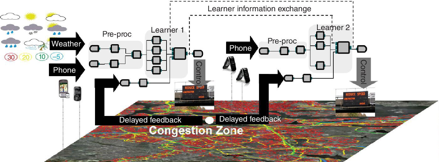
Figure 10.2 Distributed learning needed for real‐time signage update.
Data for this real‐time prediction can be gathered from many different types of sensors. In this example we consider cell phone location information from different points of interest and local weather information. This data is naturally distributed and may not be available at one central location, due to either geographical diversity or different cell phone providers owning different subsets of the data (i.e., their customers). In this simple example we consider geographic distribution of the data. The congestion prediction problem then requires deploying multiple distributed predictors that collect data from local regions and generate local predictions that are then merged to generate a more reliable final prediction. The local prediction can be about network conditions within a specific local region—for instance congestion within a particular part of the road network. The final prediction on the other hand is computed by combining these local predictions into a composite prediction about the state of the entire network.
An example with two distributed predictor applications—each depicted as a flow graph—is shown in Figure 10.2. The two different flowgraphs in this example look at different subsets of the data and implement appropriate operations for preprocessing (cleaning, denoising, merging, alignment, spatiotemporal processing, etc.), followed by operations for learning and adaptation to compute the local prediction. These are shown as the subgraphs labeled Pre‐proc and Learner, respectively. In the most general case, a collection of different models (e.g., neural networks, decision trees, etc.), trained on appropriate training data, can be used by each predictor application.
The learners receive delayed feedback about their prediction correctness after a certain amount of time (e.g., if the prediction is for 10 minutes in advance, the label is available after 10 minutes) and can use it to modify their individual models and local aggregation. Additionally, these learners also need to exchange information about their predictions across distributed locations so that they can get a more global view of the state of the network and can improve their predictions. Prediction exchange between the learners is shown on the figure using dashed lines. Finally, the predictions from the learners can be used to update digital signage in real time and potentially alert or divert traffic as necessary.
We formalize the characteristics of this online data stream processing application (SPA) in the next section and discuss how developing it requires the design of online, distributed ensemble learning frameworks, while deploying it requires being able to instantiate these frameworks on a distributed system. In the following two sections, we show how we can leverage characteristics of modern SPSs in order to build and deploy general learning frameworks that solve distributed learning problems of this type. Our intent is to showcase how this enables a whole new way of thinking about such problems and opens up several avenues for future research.
10.3 STREAM PROCESSING CHARACTERISTICS
There is a unique combination of multiple features that distinguishes SPAs from traditional data analysis paradigms, which are often batch and offline. These features can be summarized as follows:
- Streaming and In‐Motion Analysis (SIMA). SPAs need to process streaming data on the fly, as it continues to flow, in order to support real‐time, low‐latency analysis and to match the computation to the naturally streaming properties of the data. This limits the amount of prior data that can be accessed and necessitates one‐pass, online2 algorithms [6–8]. Several streaming algorithms are described in [9, 10].
- Distributed Data and Analysis (DDA). SPAs analyze data streams that are often distributed, and their large rates make it impossible to adopt centralized solutions. Hence, the applications themselves need to be distributed.
- High Performance and Scalable Analysis (HPSA). SPAs require high‐throughput, low‐latency, and dynamic scalability. This means that SPAs should be structured to exploit distributed computation infrastructures and different forms of parallelism (e.g., pipelined data and tasks). This also means that they often require joint application and system optimization [11, 12].
- Multimodal Analysis (MMA). SPAs need to process streaming information across heterogeneous data sources, including structured (e.g., transactions), unstructured (e.g., audio, video, text, image), and semi‐structured data. In our transportation example this includes sensor readings, user‐contributed text and images, traffic cameras, etc.
- Loss‐Tolerant Analysis (LTA). SPAs need to analyze lossy data with different noise levels, statistical and temporal properties, mismatched sampling rates, etc., and hence they often need appropriate processing to transform, clean, filter, and convert data and results. This also implies the need to match data rates, handle lossy data, synchronize across different data streams, and handle various protocols [7]. SPAs need to account for these issues and provide graceful degradation of results to loss in the data.
- Adaptive and Time‐Varying Analysis (ATA). SPAs are often long running and need to adapt over time to changes in the data and problem characteristics. Hence, SPAs need to support dynamic reconfiguration based on feedback, current context, and results of the analysis [6–8].
Systems and algorithms for SPAs need to provide capabilities that address these features and their combinations effectively.
10.4 DISTRIBUTED STREAM PROCESSING SYSTEMS
The signal processing and research community has so far focused on the theoretical and algorithmic issues for the design of SPAs but has had limited success in taking such applications into real‐world deployments. This is primarily due to the multiple practical considerations involved in building an end‐to‐end deployment and the lack of a comprehensive system and tools that provide them the requisite support. In this section, we summarize efforts at building systems to support SPAs and their shortcomings and then describe how current SPSs can help realize such deployments.
10.4.1 State of the Art
Several systems, combining principles from data management and distributed processing, have been developed over time to support different subsets of requirements that are now central to SPAs. These systems include traditional databases and data warehouses, parallel processing frameworks, active databases, continuous query systems, publish–subscribe (pub‐sub) systems, complex event processing (CEP) systems, and more recently the Map‐Reduce frameworks. A quick summary of the capabilities of these systems with respect to the streaming application characteristics defined in Section 10.3 is included in Table 10.1.
TABLE 10.1 Data Management Systems and Their Support for SPA Requirements
| System | SIMA | DDA | HPSA | MMA | LTA | ATA |
| Databases | No | Yes | Partly | No | Yes | No |
| (DB2, Oracle, MySQL) | ||||||
| Parallel processing | No | Yes | Yes | Yes | Yes | No |
| (PVM, MPI, OpenMP) | ||||||
| Active databases | Partly | Partly | No | No | Yes | Yes |
| (Ode, HiPac, Samos) | ||||||
| Continuous query systems | Partly | Partly | No | No | Yes | Yes |
| (NiagaraCQ, OpenCQ) | ||||||
| Pub–sub systems | Yes | Yes | No | No | Yes | Partly |
| (Gryphon, Siena, Padres) | ||||||
| CEP systems | Yes | Partly | Partly | No | Yes | Partly |
| (WBE, Tibco BE, Oracle CEP) | ||||||
| MapReduce (Hadoop) | No | Yes | Yes | Yes | Yes | No |
SIMA, Streaming and In‐Motion Analysis; DDA, Distributed Data and Analysis; HPSA, High‐Performance and Scalable Analysis; MMA, Multimodal Analysis; LTA, Loss‐Tolerant Analysis; and ATA, Adaptive and Time‐Varying Analysis.
More details on the individual systems and their examples can be obtained from Ref. [9]. However, as is clear, none of these systems were truly designed to handle all requirements of SPAs. Even the recent MapReduce paradigm does not support SIMA and ATA—critical to the needs of these types of applications. As a consequence, there is an urgent need to develop more sophisticated SPSs.
10.4.2 Stream Processing Systems
While SPSs were developed by incorporating ideas from these preceding technologies, they required several advancements to the state of the art in algorithmic, analytic, and systems concepts. These advances include sophisticated and extensible programming models, allowing continuous, incremental, and adaptive algorithms and distributed, fault‐tolerant, and enterprise‐ready infrastructures or runtimes. These systems are designed to allow end‐to‐end distribution of real‐time analysis, as needed in a fog computing world. Examples of early SPSs include TelegraphCQ, STREAM, Aurora–Borealis, Gigascope, and Streambase [9]. Currently available and widely used SPSs include IBM InfoSphere Streams [3] (streams) and open‐source Storm [4] and Spark [5] platforms. These platforms are freely available for experimentation and usage in commercial, academic, and research settings. These systems have been extensively deployed in multiple domains for telecommunication call detail record analysis, patient monitoring in ICUs, social media monitoring for real‐time sentiment extraction, monitoring of large manufacturing systems (e.g., semiconductor, oil, and gas) for process control, financial services for online trading and fraud detection, environmental and natural systems monitoring, etc. Descriptions of some of these real‐world applications can be found in Ref. [9]. These systems have also been shown to scale rates of millions of data items per second, deployed across tens of thousands of processors in a distributed cluster, provide latencies of microseconds or lower, and connect with millions of distributed sensors.
While we omit a detailed description of stream processing platforms, we illustrate some of their core capabilities and constructs to support the needs of SPAs by outlining an implementation of the transportation application described in Section 10.2 in a stream programming language (SPL). In Figure 10.2, the application is shown as a flowgraph, which captures logical flow of data from one processing stage to another. Representing an application as a flowgraph allows for modular design and construction of the implementation, and as we discuss later, it allows SPSs to optimize the deployment of the application onto distributed computational infrastructures.
Each node on the processing flowgraphs in Figure 10.2 that consumes and/or produces a stream of data is labeled an operator. Individual streams carry data items or tuples that can contain structured numeric values, unstructured text, semi‐structured content such as XML, and binary blobs. In Table 10.2 we present an outline implementation in SPL [3]. Note that this flowgraph actually implements the distributed learning framework that will be discussed in more detail in Section 10.5.
TABLE 10.2 Example of Streams Programming to Realize Congestion Prediction Application Flowgraph
|
In this code, logical composition is indicated by an operator instance stream <type> S3 = MyOp(S1;S2), where operator MyOp consumes streams S1 and S2 to produce stream S3, where type represents the type of tuples on the stream. Note that these streams may be produced and consumed on different computational resources—but that is transparent to the application developer. Systems like Streams also include multiple operators/tools that are required to build such an application. Examples include operators for:
- Data Sources and Connectors, for example,
FileSource,TCPSource,ODBCSource - Relational Processing, for example,
Join,Aggregate,Functor,Sort - Time Series Analysis, for example,
Resample,Normalize,FFT,ARIMA,GMM - Custom Extensions, for example, user‐created operators in C++/Java or wrapping for MATLAB, Python, and R code
These constructs allow for the implementation of distributed and ensemble learning techniques, such as those introduced in the learning framework, within specialized operators. We discuss this more in Section 10.5. Stream processing platforms also include special tools for geo‐spatial processing (e.g., for distance computation, map matching, speed and direction estimation, bounding box calculations) and standard mathematical processing. A more exhaustive list is available from Ref. [3].
Finally, programming constructs like the Export operator allows applications (in our case the congestion prediction application) to publish their output stream such that other applications, for example, other learners, can dynamically connect to receive these results. This construct allows for dynamic connections to be established and torn down as other learners are instantiated or choose to communicate. This is an important requirement for the learning framework in Section 10.5.
These constructs allow application developers to focus on the core algorithm design and logical flowgraph construction, while the system provides support for communication of tuples across operators, conversion of the flowgraph into a set of processes or processing elements (PEs), distribution and placement of these PEs across a distributed computation infrastructure, and finally necessary optimizations for scaling and adapting the deployed applications. We present an illustration of the process used by such systems to convert a logical flowgraph to a physical deployment in Figure 10.3.
Figure 10.3 From logical operator flowgraphs to deployment.
Among the biggest strengths of using a stream processing platform is the natural scalability and efficiency provided by these systems and their support for extensibility in terms of optimization techniques for topology construction, operator fusion, operator placement, and adaptation [9]. These systems allow users to formulate and provide additional algorithms to optimize their applications based on the application, data, and resource‐specific requirements. This opens up several new research problems related to the joint optimization of algorithms and systems. For instance, consider a simple example application with two operators. Using the Streams composition language, these operators—shown as black and white boxes in Figure 10.4—can be arranged into a parallel (task parallel) or a serial (pipelined parallel) topology to perform the same task,3 as shown in Figure 10.4. This topology can also be distributed across computational resources (shown as different sized CPUs in Figure 10.4). The right choice of topology and placement depends on the resource constraints and data characteristics and needs to be dynamically adapted over time. This requires solving a joint resource optimization problem whose solution can be realized using the controls provided by SPSs. In practice, there are several such novel optimization problems that can be formulated and solved—in this joint application–system research space. For instance, Refs. [11] and [13] discuss topology construction and optimization for non trivial compositions of operators for multi‐class classification. Additionally, these systems provide support for design of novel meta‐learning and planning‐based approaches to dynamically construct, optimize, and compose topologies of operators on these systems [14].
Figure 10.4 Possible trade‐offs with parallelism and placement.
This combination of systems and algorithms enables several other open research problems in this space of joint application–system research, especially in an online, distributed, large‐scale setting. In the next section we propose a solution to build a large‐scale online distributed ensemble learning framework that leverages the capabilities provided by SPSs (and is implemented by the code in Table 10.2) to provide solutions to the illustrative problem defined in Section 10.2.
10.5 DISTRIBUTED ONLINE LEARNING FRAMEWORKS
We now formalize the problem described in Section 10.2 and propose a novel distributed learning framework to solve it. We first review the state of the art in such research and illustrate its shortcomings. Then we describe a systematic framework for online, distributed ensemble learning well suited for SPAs. Finally, as an illustrative example, we describe how such framework can be applied to a collision detection application.
10.5.1 State of the Art
As mentioned in Section 10.3, it is important for stream processing algorithms to be online, one pass, adaptive, and distributed to operate effectively under budget constraints and to support combinations (or ensembles) of multiple techniques. Recently, there has been research that uses the aforementioned techniques for analysis, and we include a summary of some of these approaches next. We partition our review into Ensemble methods, Diffusion adaptation, and finally frameworks for distributed learning.
10.5.1.1 Ensemble Methods
Ensemble techniques [15] build and combine a collection of base algorithms (e.g., classifiers) into a joint unique algorithm (classifier). Traditional ensemble schemes for data analysis are focused on analyzing stored or completely available datasets; examples of these techniques include bagging [16] and boosting [17]. In the past decade much work has been done to develop online versions of such ensemble techniques. An online version of AdaBoost is described in Refs. [18], and similar proposals are made in Refs. [19] and [20]. Minku and Xin [21] propose a scheme based on two online ensembles, one used for system predictions, and the other one used to learn the new concept after a drift is detected. Weighted majority [22] is an ensemble technique that maintains a collection of given learners, predicts using a weighted majority rule, and decreases in a multiplicative manner the weights of the learners in the pool that disagree with the label whenever the ensemble makes a mistakes. In Ref. [23] the weights of the learners that agree with the label when the ensemble makes a mistakes are increased, and the weights of the learners that disagree with the label are decreased also when the ensemble predicts correctly. To prevent the weights of the learners that performed poorly in the past from becoming too small with respect to the other learners, Herbster and Warmuth [24] propose a modified version of weighted majority adding a phase, after the multiplicative weight update, in which each learner shares a portion of its weight with the other learners.
While many of the ensemble learning techniques have been developed assuming no a priori knowledge about the statistical properties of the data—as is required in most of the SPAs—these techniques are often designed for a centralized scenario. In fact, the base classifiers in these approaches are not distributed entities; they all observe the same data streams, and the focus of ensemble construction is on the statistical advantages of learning with an ensemble, with little study of learning under communication constraints. It is possible to cast these techniques within the framework of distributed learning, but as is they would suffer from many drawbacks. For example, Refs. [18–21] would require an entity that collects and stores all the data recently observed by the learners and that tells the learners how to adapt their local classifiers, which are clearly impractical in SPAs that need to process real‐time streams characterized by high data rates.
10.5.1.2 Diffusion Adaptation Methods
Diffusion adaptation literature [25–32] consists of learning agents that are linked together through a network topology in a distributed setting. The agents must estimate some parameters based on their local observations and on the continuous sharing and diffusion of information across the network, and there is a focus on learning in distributed environments under communication constraints. In fact, Ref. [32] shows that a classification problem can be cast within the diffusion adaptation framework. However, there are some major constraints that are posed on the learners. First, in Refs. [25–32] all the learners are required to estimate the same set of parameters (i.e., they pursue a common goal) and combine their local estimates to converge toward a unique and optimal solution. This is a strong assumption for SPAs, as the learners might have different objectives and may use different information depending on what they observe and on their spatiotemporal position in the network. Hence, the optimal aggregation function may need to be specific to each learner.
10.5.1.3 Frameworks for Distributed Learning
There has been a large amount of recent work on building frameworks for distributed online learning with dynamic data streams, limited communication, delayed labels and feedback, and self‐interested and cooperative learners [7, 33–35]. We discuss this briefly next.
To mine the correlated, high‐dimensional, and dynamic data instances captured by one or multiple heterogeneous data sources, extract actionable intelligence from these instances, and make decisions in real time as discussed previously, a few important questions need to be answered: which processing/prediction/decision rule should a local learner (LL) select? How should the LLs adapt and learn their rules to maximize their performance? How should the processing/predictions/decisions of the LLs be combined/fused by a meta‐learner to maximize the overall performance? Most literature treats the LLs as black box algorithms and proposes various fusion algorithms for the ensemble learner with the goal of issuing predictions that are at least as good as the best LL in terms of prediction accuracy, and the performance bounds proved for the ensemble in these works depend on the performance of the LLs. In Ref. [34] the authors go one step further and study the joint design of learning algorithms for both the LLs and the ensemble. They present a novel systematic learning method (Hedge Bandits), which continuously learns and adapts the parameters of both the LLs and the ensemble, after each data instance, and provide both long‐run (asymptotic) and short‐run (rate of learning) performance guarantees. Hedge Bandits consists of a novel contextual bandit algorithm for the LLs and Hedge algorithm for the ensemble and is able to exploit the adversarial regret guarantees of Hedge and the data‐dependent regret guarantees of the contextual bandit algorithm to derive a data‐dependent regret bound for the ensemble.
In Ref. [7], the ensemble learning consists of multiple‐distributed LLs, which analyze different streams of data correlated to a common classification event, and local predictions are collected and combined using a weighted majority rule. A novel online ensemble learning algorithm is then proposed to update the aggregation rule in order to adapt to the underlying data dynamics. This overcomes several limitations of prior work by allowing for (i) different correlated data streams with statistical dependency among the label and the observation being different across learners, (ii) data being processed incrementally, once on arrival leading to improved scalability, (iii) support for different types of local classifiers including support vector machine, decision tree, neural networks, offline/online classifiers, etc., and (iv) asynchronous delays between the label arrival across the different learners. A modified version of this framework was applied to the problem of collision detection by networked sensors similarly to the one that we discussed on Section 10.2 of this chapter. For details, please refer to Ref. [36].
A more general framework, where the rule for making decisions and predictions is general and depends on the costs and accuracy (specialization) of the autonomous learners, was proposed in Ref. [33]. This cooperative online learning scheme considers (i) whether the learners can improve their detection accuracy by exchanging and aggregating information, (ii) whether the learners improve the timeliness of their detections by forming clusters, that is, by collecting information only from surrounding learners, and (iii) whether, given a specific trade‐off between detection accuracy and detection delay, it is desirable to aggregate a large amount of information or it is better to focus on the most recent and relevant information.
In Ref. [37], these techniques are considered in a setting with a number of speed sensors that are spatially distributed along a street and can communicate via an exogenously determined network, and the problem of detecting in real‐time collisions that occur within a certain distance from each sensor is studied.
In Ref. [35], a novel framework for decentralized, online learning by many self‐interested learners is considered. In this framework, learners are modeled as cooperative contextual bandits, and each learner seeks to maximize the expected reward from its arrivals, which involves trading off the reward received from its own actions, the information learned from its own actions, the reward received from the actions requested of others, and the cost paid for these actions—taking into account what it has learned about the value of assistance from each other learner. A distributed online learning algorithm is provided, and analytic bounds to compare the efficiency of these algorithms with the complete knowledge (oracle) benchmark (in which the expected reward of every action in every context is known by every learner) are established: regret—the loss incurred by the algorithm—is sublinear in time. These methods have been adapted in Ref. [38] to provide expertise discovery in medical environments. Here, an expert selection system is developed that learns online who is the best expert to treat a patient having a specific condition or characteristic.
In Section 10.5.2 we describe one such framework for online, distributed ensemble learning that addresses some of the challenges discussed in Section 10.3 and is well suited for the transportation problem described in Section 10.2. The presented methodology does not require a priori knowledge of the statistical properties of the data. This means that it can be applied both when a priori information is available and when a priori information is not available. However, if the statistical properties of the data are available beforehand, it may be convenient to apply schemes that are specifically designed to take into account the known statistical properties of the data. Moreover, the presented methodology does not require any specific assumption on the form of the loss or objective function. This means that any loss or objective function can be adopted. However, notice that the final performance of scheme depends on the selected function. For illustrative purposes, in Section 10.5.3 we consider a specific loss function, and we derive an adaptive algorithm based on this loss function, and in Section 10.5.4 we describe how the proposed framework can be adopted for a collision detection application.
10.5.2 Systematic Framework for Online Distributed Ensemble Learning
We now proceed to formalize the problem of large‐scale distributed learning from heterogeneous and dynamic data streams using the problem defined in Section 10.2. Formally, we consider a set ![]() of learners that are geographically distributed and connected via links among pairs of learners. We say that there is a link (i, j) between learners i and j if they can communicate directly with each other. In the case of our congestion application, each learner observes part of the transportation network by consuming geographically local readings from sensors and phones within a region and is linked to other learner streams via interfaces like the export–import interface described in Section 10.4.
of learners that are geographically distributed and connected via links among pairs of learners. We say that there is a link (i, j) between learners i and j if they can communicate directly with each other. In the case of our congestion application, each learner observes part of the transportation network by consuming geographically local readings from sensors and phones within a region and is linked to other learner streams via interfaces like the export–import interface described in Section 10.4.
Each learner is an ensemble of local classifiers that observes a specific set of data sources and relies on them to make local classifications, that is, partition data items into multiple classes of interest.4 In our application scenario, this maps to a binary classification task—predicting presence of congestion at a certain location within a certain time window. Each local classifier may be an arbitrary function (e.g., implemented using well‐known techniques such as neural networks, decision trees, etc.) that performs classification for the classes of interest. In Table 10.2 we show an implementation of this in an SPL with two local classifiers, MySVM and MyNN operators, and an aggregate MyAggregation operator. In order to simplify the discussion, we assume that each learner exploits a single local classifier, and we focus on binary classification problems, but it is possible to generalize the approach to the multi‐classifier and multi‐class cases. Each learner is also characterized by a local aggregation rule, which is adaptive.
Raw data items in our application can include sensor readings from the transportation network and user phones, as well as information about the weather. These data items are cleaned, preprocessed, and merged, and features are extracted from them (e.g., see Table 10.2), which are then sent to the geographically appropriate learner. We assume a synchronous processing model with discrete time slots. At each time slot, each learner observes a feature vector. It first exploits the local classifier to make a local prediction for that slot, and then it sends its local prediction to other learners in its neighborhood and receives local predictions from the other learners, before it finally exploits the aggregation rule to combine its local predictions and the predictions from its neighbors into a final classification.
Consider a discrete time model in which time is divided into slots, but an extension to a continuous time model is possible. At the beginning of the n‐th time slot, K multidimensional instances ![]() ,
, ![]() , and K labels
, and K labels ![]() ,
, ![]() , are drawn from an underlying and unknown joint probability distribution. Each learner i observes the instance
, are drawn from an underlying and unknown joint probability distribution. Each learner i observes the instance ![]() , and its task is to predict the label
, and its task is to predict the label ![]() (see Figure 10.6). We shall assume that a label
(see Figure 10.6). We shall assume that a label ![]() is correlated with all the instances
is correlated with all the instances ![]() ,
, ![]() . In this way, learner i’s observation can contain information about the label that learner j has to predict. We remark that this correlation is not known beforehand.
. In this way, learner i’s observation can contain information about the label that learner j has to predict. We remark that this correlation is not known beforehand.
Each learner i is equipped with a local classifier ![]() that generates the local prediction
that generates the local prediction ![]() based on the observed instance
based on the observed instance ![]() at time slot n. Our framework can accommodate both static pre‐trained classifiers and adaptive classifiers that learn online the parameters and configurations to adopt [39]. However, the focus of this section will not be on classifier design, for which many solutions already exist (e.g., support vector machines, decision trees, neural networks, etc.); instead, we will focus on how the learners exchange and learn how to aggregate the local predictions generated by the classifiers.
at time slot n. Our framework can accommodate both static pre‐trained classifiers and adaptive classifiers that learn online the parameters and configurations to adopt [39]. However, the focus of this section will not be on classifier design, for which many solutions already exist (e.g., support vector machines, decision trees, neural networks, etc.); instead, we will focus on how the learners exchange and learn how to aggregate the local predictions generated by the classifiers.
We allow the distributed learners to exchange and aggregate their local predictions through multihop communications; however, within one time slot a learner can send only a single transmission to each of its neighbors. We denote by ![]() learner j’s local prediction possessed by learner i before the aggregation at time instant n. The information is disseminated in the network as follows. First, each learner i observes
learner j’s local prediction possessed by learner i before the aggregation at time instant n. The information is disseminated in the network as follows. First, each learner i observes ![]() and updates
and updates ![]() . Next, learner i transmits to each neighbor j the local prediction
. Next, learner i transmits to each neighbor j the local prediction ![]() and the local predictions
and the local predictions ![]() , for each learner
, for each learner ![]() such that the link (i, j) belongs to the shortest path between k and j. Hence, if transmissions are always correctly received, we have
such that the link (i, j) belongs to the shortest path between k and j. Hence, if transmissions are always correctly received, we have ![]() and
and ![]() ,
, ![]() , where d
ij
is the distance in number of hops between i and j. For instance, Figure 10.5 represents the flow of information toward learner 1 for a binary tree network assuming that transmissions are always correctly received. More generally, if transmissions can be affected by communication errors, we have
, where d
ij
is the distance in number of hops between i and j. For instance, Figure 10.5 represents the flow of information toward learner 1 for a binary tree network assuming that transmissions are always correctly received. More generally, if transmissions can be affected by communication errors, we have ![]() , for some
, for some ![]() .
.
Figure 10.5 Flow of information toward learner 1 at time slot n for a binary tree network.
Each learner i employs a weighted majority aggregation rule to fuse the data it possesses and generates a final prediction ![]() as follows:
as follows:
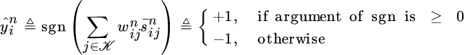
where ![]() is the sign function. In the example earlier, we use a threshold of 0 on the value of the argument to separate the two classes. In practice this threshold can be arbitrary; however this does not affect the discussion next, as the threshold corresponds to a constant shift in the argument.
is the sign function. In the example earlier, we use a threshold of 0 on the value of the argument to separate the two classes. In practice this threshold can be arbitrary; however this does not affect the discussion next, as the threshold corresponds to a constant shift in the argument.
In the earlier construction, learner i first aggregates all possessed predictions ![]() using the weights
using the weights ![]() and then uses the sign of the fused information to output its final classification,
and then uses the sign of the fused information to output its final classification, ![]() . While weighted majority aggregation rules have been considered before in the ensemble learning literature [17– 20], there is an important distinction in Equation (10.1) that is particularly relevant to the online distributed stream mining context: since we are limiting the learners to exchange information only via links, learners receive information from other learners with delay (i.e., in general
. While weighted majority aggregation rules have been considered before in the ensemble learning literature [17– 20], there is an important distinction in Equation (10.1) that is particularly relevant to the online distributed stream mining context: since we are limiting the learners to exchange information only via links, learners receive information from other learners with delay (i.e., in general ![]() ), as a consequence different learners have different information to exploit (i.e., in general
), as a consequence different learners have different information to exploit (i.e., in general ![]() ).
).
Each learner i maintains a total of K weights and K local predictions, which we collect into vectors:
Given the weight vector ![]() , the decision rule (10.1) allows for a geometric interpretation: the homogeneous hyperplane in ℜ
K
that is orthogonal to
, the decision rule (10.1) allows for a geometric interpretation: the homogeneous hyperplane in ℜ
K
that is orthogonal to ![]() separates the positive prediction (i.e.,
separates the positive prediction (i.e., ![]() ) from the negative predictions (i.e.,
) from the negative predictions (i.e., ![]() ).
).
We consider an online learning setting in which the true label ![]() is eventually observed by learner i. Learner i can then compare both
is eventually observed by learner i. Learner i can then compare both ![]() and
and ![]() and use this information to update the weights it assigns to the other learners. Indeed, since we do not assume any a priori information about the statistical properties of the processes that generate the data observed by the various learners, we can only exploit the available observations and the history of past data to guide the design of the adaptation process over the network.
and use this information to update the weights it assigns to the other learners. Indeed, since we do not assume any a priori information about the statistical properties of the processes that generate the data observed by the various learners, we can only exploit the available observations and the history of past data to guide the design of the adaptation process over the network.
In summary, the sequence of events that takes place in a generic time slot n, represented in Figure 10.6, involves five phases:
Figure 10.6 System model described in Section 10.5.2.
-
Observation. Each learner i observes an instance
 at time n.
 - Information Dissemination. Learners send the local predictions they possess to their neighbors.
-
Final Prediction. Each learner i computes and outputs its final prediction
 .
. -
Feedback. Learners can observe the true label
 that refers to a time slot
  .
. -
Adaptation. If
 is observed, learner i updates its aggregation vector from
  to
to  .
.
In the context of the discussed framework, it is fundamental to develop strategies for adapting the aggregation weights ![]() over time, in response to how well the learners perform. A possible approach is discussed next.
over time, in response to how well the learners perform. A possible approach is discussed next.
10.5.3 Online Learning of the Aggregation Weights
A possible approach to update the aggregation weights is to associate with each learner i an instantaneous loss function ![]() and minimize, with respect to the weight vector w
i
, the cumulative loss given all observations up to time slot n. In the following we consider this approach, adopting an instantaneous hinge loss function [40]:
and minimize, with respect to the weight vector w
i
, the cumulative loss given all observations up to time slot n. In the following we consider this approach, adopting an instantaneous hinge loss function [40]:
For each time instant n, we consider the one‐shot loss function
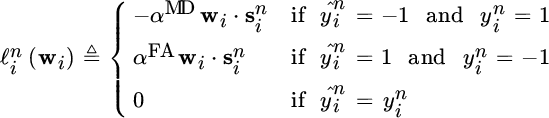
where the parameters ![]() and
and ![]() are the mis‐detection and false alarm unit costs and
are the mis‐detection and false alarm unit costs and ![]() denotes the scalar product between w
i
and
denotes the scalar product between w
i
and ![]() . The hinge loss function is equal to 0 if the weight vector w
i
allows to predict correctly the label
. The hinge loss function is equal to 0 if the weight vector w
i
allows to predict correctly the label ![]() ; otherwise the value of the loss function is proportional to the distance of
; otherwise the value of the loss function is proportional to the distance of ![]() from the separating hyperplane defined by w
i
, multiplied by α
MD if the prediction is
from the separating hyperplane defined by w
i
, multiplied by α
MD if the prediction is ![]() but the label is 1, we refer to this type of error as a mis‐detection, or multiplied by α
FA if the prediction is 1 but the label is
but the label is 1, we refer to this type of error as a mis‐detection, or multiplied by α
FA if the prediction is 1 but the label is ![]() , we refer to this type of error as a false alarm.
, we refer to this type of error as a false alarm.
The hinge loss function gives higher importance to errors that are more difficult to correct with the current weight vector. A related albeit different approach is adopted in AdaBoost [17], in which the importance of the errors increases exponentially in the distance of the local prediction vector from the separating hyperplane. Here, however, the formulation is more general and allows for the diffusion of information across neighborhoods simultaneously, as opposed to assuming each learner has access to information from across the entire set of learners in the network.
We can then formulate a global objective for the distributed stream mining problem as that of determining the optimal weights by minimizing the cumulative loss given all observations up to time slot n:
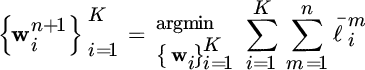
where ![]() if
if ![]() has been observed by time instant n, otherwise
has been observed by time instant n, otherwise ![]() .
.
To solve (10.4) learner i must store all previous labels and all previous local predictions of all the learners in the system, which is impractical in SPAs, where the volume of the incoming data is high and the number of learners is large. Hence, we adopt the stochastic gradient descent algorithm to incrementally approach the solution of (10.4) using only the most recently observed label. If label ![]() is observed at the end of time instant n, we obtain the following update rule for
is observed at the end of time instant n, we obtain the following update rule for ![]() :
:
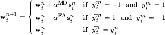
where ![]() is the prediction that learner i would have made at time instant m with the current weight vector
is the prediction that learner i would have made at time instant m with the current weight vector ![]() . This construction allows a meaningful interpretation. It shows that learner i should maintain its level of confidence in its data when its decision agrees with the observed label. If disagreement occurs, then learner i needs to assess which local predictions lead to the misclassification: the weight
. This construction allows a meaningful interpretation. It shows that learner i should maintain its level of confidence in its data when its decision agrees with the observed label. If disagreement occurs, then learner i needs to assess which local predictions lead to the misclassification: the weight ![]() that learner i adopts to scale the local predictions it receives from learner j is increased (by either α
MD or α
FA units, depending on the type of error) if the local prediction sent by j agreed with the label, otherwise
that learner i adopts to scale the local predictions it receives from learner j is increased (by either α
MD or α
FA units, depending on the type of error) if the local prediction sent by j agreed with the label, otherwise ![]() is decreased.
is decreased.
[?] and [8] derive worst‐case upper bounds for the misclassification probability of a learner adopting the update rule 10.5. Such bounds are expressed in terms of the misclassification probabilities of two benchmarks: (i) the misclassification probability of the best local classifiers and (ii) the misclassification probability of the best linear aggregator. We remark that the best local classifiers and the best linear aggregator are not known and cannot be computed beforehand; in fact, this would require to know in advance the realization of the process that generates the instances and the labels.
The optimization problem (10.4) can also be solved within the diffusion adaptation framework, as proposed in Ref. [32]. In this framework the learners combine information with their neighbors, for example, in the combine‐then‐adapt (CTA) diffusion scheme, they first combine their weights and then adopt the stochastic gradient descent [32]. Figure 10.7 illustrates the difference between our approach and the CTA scheme.
Figure 10.7 A comparison between the proposed algorithm and the combine‐then‐adapt (CTA) scheme in terms of information dissemination and weight update rule. Unlike diffusion, in the proposed approach the weight vectors do not need to be disseminated.
We remark that the framework described so far requires each learner to maintain a weight (i.e., an integer value) and a local prediction (i.e., a Boolean value) for each other learner in the network. This means that the memory and computational requirements scale linearly in the number of learners K. However, notice that the aggregation rule 10.1 and the update rule 10.5 only require basic operations such as add, multiply, and compare. Moreover, if the learners have a common goals, that is, they must predict a common class label y n , it is possible to develop a scheme in which each learner keeps track only of its own local prediction and of the weight used to scale its local prediction and is responsible to update such a weight. In this scheme the learners exchange the weighted local predictions instead of the local predictions and the memory and computational requirements scale as a constant in the number of learners K. For additional details, we refer the reviewer to Ref. [8].
The framework discussed in this subsection naturally maps onto a deployment using an SPS. Each of the learners shown in Figure 10.6 maps onto the subgraph labeled learner in Figure 10.2, with the local classifiers mapping onto the shown parallel topology and the aggregation rule mapping to the fan‐in on that subgraph. As mentioned earlier, the base classifiers may be implemented using the toolkits provided by systems like Streams that include wrappers for R and MATLAB. The feedback ![]() corresponds to the delayed feedback in Figure 10.2, and the input feature vector
corresponds to the delayed feedback in Figure 10.2, and the input feature vector ![]() is computed by the Pre‐proc part of the subgraph in Figure 10.2 and can include different types of spatiotemporal processing and feature extraction. Finally, the communication between the learners in Figure 10.6 is enabled by the learner information exchange connections in Figure 10.2. In summary, this online, distributed ensemble learning framework can naturally be implemented on a stream processing platform. This combination is very powerful, as it now allows the design, development, and deployment of such large‐scale complex applications much more feasible, and it also enables a range of novel signal processing, optimization, and scheduling research. We discuss some of these open problems in Section 10.6.
is computed by the Pre‐proc part of the subgraph in Figure 10.2 and can include different types of spatiotemporal processing and feature extraction. Finally, the communication between the learners in Figure 10.6 is enabled by the learner information exchange connections in Figure 10.2. In summary, this online, distributed ensemble learning framework can naturally be implemented on a stream processing platform. This combination is very powerful, as it now allows the design, development, and deployment of such large‐scale complex applications much more feasible, and it also enables a range of novel signal processing, optimization, and scheduling research. We discuss some of these open problems in Section 10.6.
10.5.4 Collision Detection Application
In this subsection we apply the framework described in Sections 10.5.2 and 10.5.3 to a collision detection application in which a set of speed sensors—which are spatially distributed along a street—must detect in real‐time collisions that occur within a certain distance from them.
We consider a set ![]() of K speed sensors that are distributed along both travel directions of a street (see the left side of Figure 10.8). We focus on a generic sensor i that must detect the occurrence of collision events within z miles from its location along the corresponding travel direction, where z is a predetermined parameter. A collision event e
ℓ
is characterized by an unknown starting time t
ℓ,start, when the collision occurs, and an unknown ending time t
ℓ,end, when the collision is cleared. The goal of sensor i is to detect the collision e
ℓ
by the time
of K speed sensors that are distributed along both travel directions of a street (see the left side of Figure 10.8). We focus on a generic sensor i that must detect the occurrence of collision events within z miles from its location along the corresponding travel direction, where z is a predetermined parameter. A collision event e
ℓ
is characterized by an unknown starting time t
ℓ,start, when the collision occurs, and an unknown ending time t
ℓ,end, when the collision is cleared. The goal of sensor i is to detect the collision e
ℓ
by the time ![]() , where T
max can be interpreted as the maximum time after the occurrence of the collision such that the information about the collision occurrence can be exploited to take better informed actions (e.g., the average time after which a collision is reported by other sources).
, where T
max can be interpreted as the maximum time after the occurrence of the collision such that the information about the collision occurrence can be exploited to take better informed actions (e.g., the average time after which a collision is reported by other sources).
Figure 10.8
A generic speed sensor i must detect collisions in real time and inform the drivers (left). To achieve this goal sensor i receives the observations from the other sensors, and the flow of information is represented by a directed graph  (right).
We divide the time into slots of length T. We write ![]() if a collision occurs at or before time instant n and is not cleared by time instant n, whereas we write
if a collision occurs at or before time instant n and is not cleared by time instant n, whereas we write ![]() to represent the absence of a collision. Figure 10.9 illustrates these notations.
to represent the absence of a collision. Figure 10.9 illustrates these notations.
Figure 10.9 Illustration of the considered notations.
At the beginning of the n‐th time slot, each speed sensor j observes a speed value ![]() , which represents the average speed value of the cars that have passed through sensor j from the beginning of the
, which represents the average speed value of the cars that have passed through sensor j from the beginning of the ![]() ‐th time slot until the beginning of the n‐th time slot. We consider a threshold‐based classifier:
‐th time slot until the beginning of the n‐th time slot. We consider a threshold‐based classifier:
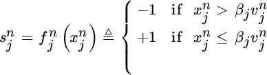
where ![]() is the average speed observed by sensor j during that day of the week and time of the day, and
is the average speed observed by sensor j during that day of the week and time of the day, and ![]() is a threshold parameter.
is a threshold parameter.
If sensor j is close to sensor i, the speed value ![]() and the local prediction
and the local prediction ![]() are correlated to the occurrence or absence of the collision events that sensor i must detect. For this reason, to detect collisions in an accurate and timely manner, the sensors must exchange their local predictions. Specifically, we denote the sensors such that sensor i precedes sensor
are correlated to the occurrence or absence of the collision events that sensor i must detect. For this reason, to detect collisions in an accurate and timely manner, the sensors must exchange their local predictions. Specifically, we denote the sensors such that sensor i precedes sensor ![]() in the direction of travel. In order to detect whether a collision has occurred within z miles from its location, sensor i requires the observations of the subsequent sensors in the direction of travel (e.g., sensors
in the direction of travel. In order to detect whether a collision has occurred within z miles from its location, sensor i requires the observations of the subsequent sensors in the direction of travel (e.g., sensors ![]() ,
, ![]() , etc.) up to the sensor that is far from sensor i more than z miles. Hence, the information flows in the opposite direction with respect to the direction of travel. Such a scenario is represented by the right side of Figure 10.8. Notice that sensor
, etc.) up to the sensor that is far from sensor i more than z miles. Hence, the information flows in the opposite direction with respect to the direction of travel. Such a scenario is represented by the right side of Figure 10.8. Notice that sensor ![]() is responsible to collect the observation from sensor
is responsible to collect the observation from sensor ![]() and to send to sensor i both its observation and the observation of
and to send to sensor i both its observation and the observation of ![]() .
.
Figure 10.8 shows also the flow of information provided by one side of the street to the other side of the street (i.e., from sensor k to sensor i). Indeed, the fact that the observations on one side of the street are not influenced by a collision on the other side of the street can be extremely useful to assess the traffic situation and distinguish between collisions and other types of incidents. For example, the sudden decrease of the speed observed by some sensors in the considered travel direction may be a collision warning sign; however, if at the same time instants the speed observed by the sensors in the opposite travel direction decreases as well, then an incident that affect both travel directions may have occurred (e.g., it started to rain) instead of a collision.
We can formally define the flow of information represented by the right side of Figure 10.8 with a directed graph ![]() ,5 where
,5 where ![]() is the subset of sensors that send their local predictions to sensor i (included i itself) and
is the subset of sensors that send their local predictions to sensor i (included i itself) and ![]() is the set of links among pairs of sensors.
is the set of links among pairs of sensors.
Now both the local classifiers and the flow of information are defined, learner i can adopt the framework described in Sections 10.5.2 and 10.5.3 to detect the occurrence of collisions within z miles from its location. Specifically, learner i maintains in memory K
i
weights (K
i
is the cardinality of ![]() ) that are collected in the weight vector
) that are collected in the weight vector ![]() ; it predicts adopting 10.1 and it updates the weights adopting 10.5 whenever a feedback is received. The feedback about the occurrence of the collision event e
ℓ
can be provided, for example, by a driver or by a police officer, and it is in general received with delay. In Figure 10.8 such a delay is denoted by Z
ℓ
.
; it predicts adopting 10.1 and it updates the weights adopting 10.5 whenever a feedback is received. The feedback about the occurrence of the collision event e
ℓ
can be provided, for example, by a driver or by a police officer, and it is in general received with delay. In Figure 10.8 such a delay is denoted by Z
ℓ
.
We have evaluated the proposed framework over real‐word datasets. Specifically, we have exploited a dataset containing the speed readings of the loop sensors that are distributed along a 50 mile segment of the freeway 405 that passes through Los Angeles County and a collision dataset containing the reported collisions that occurred along the freeway 405 during the months of September, October, and November 2013. For a more detailed description of the datasets, we refer the reader to Ref. [41]. Our illustrative results show that the considered framework is able to detect more than half of the collisions occurring within a distance of 4 miles from a specific sensors while generating false alarms in the order of one false alarm every 100 predictions. The results show also that by setting the ratio α MD/α FA, mis‐detections and false alarms can be traded off.
10.6 WHAT LIES AHEAD
There are several open research problems at this application–algorithm systems interface—needed for fog computing—that are worth investigating. First, there is currently no principled approach to decompose an online distributed large‐scale learning problem into a topology/flowgraph of streaming operators and functions. While standard engineering principles of modularity, reuse, atomicity, etc. apply, there is no formalism that supports such a decomposition.
Second, there are several optimization problems related to mapping a given processing topology onto physical processes that can be instantiated on a distributed computation platform. This requires a multi‐objective optimization where communication costs need to be traded off with memory and computational costs while ensuring efficient utilization of resources. Also, given that resource requirements and data characteristics change over time, these optimization problems may need to be solved incrementally or periodically. The interaction between these optimizations and the core learning problem needs to be also formally investigated.
Third, there are several interesting topology configuration and adaptation problems that can be considered: learners can be dynamically switched on or off to reduce system resource usage or improve system performance; the topology through which they are connected can adapt to increase parallelism; the selectivity operating points of individual classifiers can be modified to reduce workloads on downstream operators; past data and observations can be dynamically dropped to free memory resources; etc. The impact of each individual adaptation and of the interaction among different levels of adaptation is unclear and needs to be investigated. Some examples of exploiting these trade‐offs have been considered in Ref. [11], but this is a fertile space for future research.
Another important extension is the use of active learning approaches [42] to gather feedback in cases where it is sparse, hard, or costly to acquire.
Fourth, there is need to extend the meta‐learning aggregation rule from a linear form to other forms (e.g., decision trees) to exploit the decision space more effectively. Additionally, meta‐learners may themselves be hierarchically layered into multiple levels—with different implications for learning, computational complexity, and convergence.
Fifth, in the presence of multiple learners, potentially belonging to different entities, these ensemble approaches need to handle noncooperative and in some cases even malicious entities. In Ref. [43], a few steps have been taken in this direction. This work studies distributed online recommender systems, in which multiple learners, which are self‐interested and represent different companies/products, are competing and cooperating to jointly recommend products to users based on their search query as well as their specific background including history of bought items, gender, and age.
Finally, while we have posed the problem of distributed learning in a supervised setting (i.e., the labels are eventually observed), there is also a need to build large‐scale online algorithms for knowledge discovery in semi‐supervised and unsupervised settings. Constructing online ensemble methods for clustering, outlier detection, and frequent pattern mining are interesting directions. A few steps in these directions have been taken in Refs. [44] and [45], where context‐based unsupervised ensemble learning was proposed and clustering, respectively.
More discussion of such complex applications built on a stream processing platform, open research problems, and a more detailed literature survey may be obtained from Ref. [9]. Overall, we believe that the space of distributed, online, large‐scale ensemble learning using stream processing middleware is an extremely fertile space for novel research and construction of real‐world deployments that have the potential to accelerate our effective use of streaming Big Data to realize a Smarter Planet.
ACKNOWLEDGMENT
The authors would like to acknowledge the Air Force DDAS Program for support.
REFERENCES
- 1. “IBM Smarter Planet,” http://www.ibm.com/smarterplanet (accessed September 24, 2016), retrieved October 2012.
- 2. “ITU Report: Measuring the Information Society,” http://www.itu.int/dms_pub/itu‐d/opb/ind/D‐IND‐ICTOI‐2012‐SUM‐PDF‐E.pdf (accessed September 24, 2016), 2012.
- 3. “IBM InfoSphere Streams,” www.ibm.com/software/products/en/infosphere‐streams/ (accessed September 24, 2016), retrieved March 2011.
- 4. “Storm Project,” http://storm‐project.net/ (accessed September 24, 2016), retrieved October 2012.
- 5. “Apache Spark,” http://spark.apache.org/ (accessed September 24, 2016), retrieved September 2015.
- 6. Y. Zhang, D. Sow, D. S. Turaga, and M. van der Schaar, “A fast online learning algorithm for distributed mining of big data,” in The Big Data Analytics Workshop at SIGMETRICS, Pittsburgh, PA, USA, June 2013.
- 7. L. Canzian, Y. Zhang, and M. van der Schaar, “Ensemble of distributed learners for online classification of dynamic data streams,” IEEE Transactions on Signal and Information Processing over Networks, vol. 1, no. 3, pp. 180–194, 2015.
- 8. J. Xu, C. Tekin, and M. van der Schaar, “Distributed multi‐agent online learning based on global feedback,” IEEE Transactions on Signal Processing, vol. 63, no. 9, pp. 2225–2238, 2015.
- 9. H. Andrade, B. Gedik, and D. Turaga, Fundamentals of Stream Processing: Application Design, Systems, and Analytics. Cambridge University Press, Cambridge, 2014.
- 10. C. Aggarwal, Ed., Data Streams: Models and Algorithms. Kluwer Academic Publishers, Norwell, 2007.
- 11. R. Ducasse, D. S. Turaga, and M. van der Schaar, “Adaptive topologic optimization for large‐scale stream mining,” IEEE Journal of Selected Topics in Signal Processing, vol. 4, no. 3, pp. 620–636, 2010.
- 12. S. Ren and M. van der Schaar, “Efficient resource provisioning and rate selection for stream mining in a community cloud,” IEEE Transactions on Multimedia, vol. 15, no. 4, pp. 723–734, 2013.
- 13. F. Fu, D. S. Turaga, O. Verscheure, M. van der Schaar, and L. Amini, “Configuring competing classifier chains in distributed stream mining systems,” IEEE Journal of Selected Areas in Communications, vol. 1, no. 4, pp. 548–563, 2007.
- 14. A. Beygelzimer, A. Riabov, D. Sow, D. S. Turaga, and O. Udrea, “Big data exploration via automated orchestration of analytic workflows,” in USENIX International Conference on Automated Computing, June 26–28, 2013, San Jose, CA, 2013.
- 15. Z. Haipeng, S. R. Kulkarni, and H. V. Poor, “Attribute‐distributed learning: Models, limits, and algorithms,” IEEE Transactions on Signal Processing, vol. 59, no. 1, pp. 386–398, 2011.
- 16. L. Breiman, “Bagging predictors,” Machine Learning, vol. 24, no. 2, pp. 123–140, 1996.
- 17. Y. Freund and R. E. Schapire, “A decision‐theoretic generalization of on‐line learning and an application to boosting,” Journal of Computer and System Sciences, vol. 55, no. 1, pp. 119–139, 1997.
- 18. W. Fan, S. J. Stolfo, and J. Zhang, “The application of AdaBoost for distributed, scalable and on‐line learning,” in Proceedings of ACM SIGKDD, San Diego, CA, USA, August 1999, pp. 362–366.
- 19. H. Wang, W. Fan, P. S. Yu, and J. Han, “Mining concept‐drifting data streams using ensemble classifiers,” in Proceedings of ACM SIGKDD, Washington DC, USA, August 2003, pp. 226–235.
- 20. M. M. Masud, J. Gao, L. Khan, J. Han, and B. Thuraisingham, “Integrating novel class detection with classification for concept‐drifting data streams,” in Proceedings of ECML PKDD, Bled, Slovenia, September 2009, pp. 79–94.
- 21. L. L. Minku and Y. Xin, “DDD: A new ensemble approach for dealing with concept drift,” IEEE Transactions on Knowledge and Data Engineering, vol. 24, no. 4, pp. 619–633, 2012.
- 22. N. Littlestone and M. K. Warmuth, “The weighted majority algorithm,” Information and Computation, vol. 108, no. 2, pp. 212–261, 1994.
- 23. A. Blum, “Empirical support for winnow and weighted‐majority algorithms: Results on a calendar scheduling domain,” Machine Learning, vol. 26, no. 1, pp. 5–23, 1997.
- 24. M. Herbster and M. K. Warmuth, “Tracking the best expert,” Machine Learning, vol. 32, no. 2, pp. 151–178, 1998.
- 25. A. Ribeiro and G. B. Giannakis, “Bandwidth‐constrained distributed estimation for wireless sensor networks‐part I: Gaussian case,” IEEE Transactions on Signal Processing, vol. 54, no. 3, pp. 1131–1143, 2006.
- 26. A. Ribeiro and G. B. Giannakis, “Bandwidth‐constrained distributed estimation for wireless sensor networks‐part II: Unknown probability density function,” IEEE Transactions on Signal Processing, vol. 54, no. 7, pp. 2784–2796, 2006.
- 27. J.‐J. Xiao, A. Ribeiro, Z.‐Q. Luo, and G. B. Giannakis, “Distributed compression estimation using wireless sensor networks,” IEEE Signal Processing Magazine, vol. 23, no. 4, pp. 27–41, 2006.
- 28. J. B. Predd, S. R. Kulkarni, and H. V. Poor, “Distributed learning for decentralized inference in wireless sensor networks,” IEEE Transactions on Signal Processing, vol. 23, no. 4, pp. 56–69, 2006.
- 29. H. Zhang, J. Moura, and B. Krogh, “Dynamic field estimation using wireless sensor networks: Tradeoffs between estimation error and communication cost,” IEEE Transactions on Signal Processing, vol. 57, no. 6, pp. 2383–2395, 2009.
- 30. S. Barbarossa and G. Scutari, “Decentralized maximum‐likelihood estimation for sensor networks composed of nonlinearly coupled dynamical systems,” IEEE Transactions on Signal Processing, vol. 55, no. 7, pp. 3456–3470, 2007.
- 31. A. Sayed, S.‐Y. Tu, J. Chen, X. Zhao, and Z. Towfic, “Diffusion strategies for adaptation and learning over networks: An examination of distributed strategies and network behavior,” IEEE Signal Processing Magazine, vol. 30, no. 3, pp. 155–171, 2013.
- 32. Z. J. Towfic, J. Chen, and A. H. Sayed, “On distributed online classification in the midst of concept drifts,” Neurocomputing, vol. 112, pp. 139–152, 2013.
- 33. L. Canzian and M. van der Schaar, “Timely event detection by networked learners,” IEEE Transactions on Signal Processing, vol. 63, no. 5, pp. 1282–1296, 2015.
- 34. C. Tekin and M. van der Schaar, “Active learning in context‐driven stream mining with an application to image mining,” IEEE Transactions on Image Processing, vol. 24, no. 11, pp. 3666–3679, 2015.
- 35. C. Tekin and M. van der Schaar, “Distributed online learning via cooperative contextual bandits,” IEEE Transactions on Signal Processing, vol. 63, no. 14, pp. 3700–3714, 2015.
- 36. L. Canzian, U. Demiryurek, and M. van der Schaar, “Collision detection by networked sensors,” IEEE Transactions on Signal and Information Processing over Networks, vol. 2, no. 1, pp. 1–15, 2016.
- 37. J. Xu, D. Deng, U. Demiryurek, C. Shahabi, and M. van der Schaar, “Mining the situation: Spatiotemporal traffic prediction with big data,” IEEE Journal on Selected Topics in Signal Processing, vol. 9, no. 4, pp. 702–715, 2015.
- 38. C. Tekin, O. Atan, and M. van der Schaar, “Discover the expert: Context‐adaptive expert selection for medical diagnosis,” IEEE Transactions on Emerging Topics in Computing, vol. 3, no. 2, pp. 220–234, 2015.
- 39. D. Shutin, S. R. Kulkarni, and H. V. Poor, “Incremental reformulated automatic relevance determination,” IEEE Transactions on Signal Processing, vol. 60, no. 9, pp. 4977–4981, 2012.
- 40. L. Rosasco, E. D. Vito, A. Caponnetto, M. Piana, and A. Verri, “Are loss functions all the same?” Neural Computation, vol. 16, no. 5, pp. 1063–1076, 2004.
- 41. B. Pan, U. Demiryurek, C. Gupta, and C. Shahabi, “Forecasting spatiotemporal impact of traffic incidents on road networks,” in IEEE ICDM, Dallas, TX, USA, December 2013.
- 42. M.‐F. Balcan, S. Hanneke, and J. W. Vaughan, “The true sample complexity of active learning,” Machine Learning, vol. 80, no. 2–3, pp. 111–139, 2010.
- 43. C. Tekin, S. Zhang, and M. van der Schaar, “Distributed online learning in social recommender systems,” IEEE Journal of Selected Topics in Signal Processing, vol. 8, no. 4, pp. 638–652, 2014.
- 44. E. Soltanmohammadi, M. Naraghi‐Pour, and M. van der Schaar, “Context‐based unsupervised data fusion for decision making,” in International Conference on Machine Learning (ICML), Lille, France, July 2015.
- 45. D. Katselis, C. Beck, and M. van der Schaar, “Ensemble online clustering through decentralized observations,” in CDC, Los Angeles, CA, USA, December 2014.