Chapter 8: Additional Regressors

In your first model in Chapter 2, Getting Started with Facebook Prophet, you forecasted carbon dioxide levels at Mauna Loa, using only the date, but no other information, to predict future values. Later, in Chapter 5, Holidays, you learned how to add holidays as additional information to further refine your predictions of bicycle ridership in the Divvy bike share network in Chicago.

The way holidays are implemented in Prophet is actually a special case of adding a binary regressor. In fact, Prophet includes a generalized method for adding any additional regressor, both binary and continuous.

In this chapter, you'll enrich your Divvy dataset with weather information by including it as an additional regressor. First, you will add binary weather conditions to describe the presence or absence of sun, clouds, or rain, and then next you will bring in continuous temperature measurements. Using additional regressors can allow you to include more information to inform your models, which leads to greater predictive power. In this chapter, you will learn about the following topics:

• Adding binary regressors
• Adding continuous regressors
• Interpreting the regressor coefficients

Technical requirements

The data files and code for examples in this chapter can be found at https://github.com/PacktPublishing/Forecasting-Time-Series-Data-with-Facebook-Prophet.

Adding binary regressors

The first thing to consider with additional regressors, whether binary or continuous, is that you must have known future values for your entire forecast period. This isn't a problem with holidays because we know exactly when each future holiday will occur. All future values must either be known, as with holidays, or must have been forecast themselves separately. You must be careful though when building a forecast using data that itself has been forecast: the error in the first forecast will compound the error in the second forecast, and the errors will continuously pile up.

If one variable is much easier to forecast than another, however, then this may be a case where these stacked forecasts do make sense. A hierarchical time series is an example case where this may be useful: you may find good results by forecasting the more reliable daily values of one time series, for instance, and using those values to forecast hourly values of another time series that is more difficult to predict.

In the examples in this chapter, we are going to use a weather forecast to enrich our Divvy forecast. This additional regressor is possible because we generally do have decent weather forecasts available looking ahead a week or so. In other examples in this book, in which we have used Divvy data, we often forecasted out a full year. In this chapter though, we will only forecast out 2 weeks. Let's be generous to Chicago's weather forecasters and assume that they'll provide accurate forecasts in this time frame.

To begin, let's import our necessary packages and load the data:

import pandas as pd

import matplotlib.pyplot as plt

from fbprophet import Prophet

df = pd.read_csv('divvy_daily.csv')

Please refer to Figure 4.6 in Chapter 4, Seasonality, for a plot of the rides per day in this data. Figure 4.7 in Chapter 4, Seasonality, showed an excerpt of the data contained in this file. So far in this book, we always excluded the two columns for weather and temperature in this dataset, but we'll use them this time around. For our first example, let's consider the weather conditions. By counting the number of times each condition occurred in the dataset, we can see their frequencies:

print(df.groupby('weather')['weather'].count())

The output of the preceding print statement is as follows:

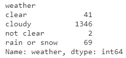
Figure 8.1 – Count of weather conditions in the Divvy dataset

By grouping the data by weather and aggregating by count, we can see the number of days each condition was reported. clear weather occurred on 41 days, and cloudy weather was by far the most common, with 1346 occurrences. not clear was only reported twice, and rain or snow 69 times.

Now that we understand what data we're working with, let's load it into our DataFrame. We'll also load the temperature column even though we won't use it until the next example when we look at continuous columns, those in which the value may exist along a continuum.

To load the weather column, we will use pandas' get_dummies method to convert it into four binary columns for each unique weather condition, meaning that each column will be a 1 or a 0, essentially a flag indicating whether the condition is present:

df['date'] = pd.to_datetime(df['date'])

df.columns = ['ds', 'y', 'temp', 'weather']

df = pd.get_dummies(df, columns=['weather'], prefix='',

                    prefix_sep='')

We can display the first five rows of our DataFrame at this point to see what the preceding code has done:

df.head()

The output of the head statement should appear as follows:

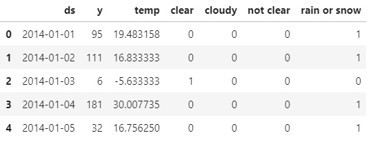
Figure 8.2 – DataFrame with dummy weather columns

You can now see that each unique value in the weather column has been converted to a new column. Let's instantiate our model now, setting the seasonality mode to multiplicative and the yearly seasonality to have a Fourier order of 4, as we did in previous chapters.

We will also add in our additional regressors using the add_regressor method. As arguments to this method, you must pass the name of the regressor, which is the name of the corresponding column in your DataFrame. You may also use the prior_scale argument to regularize the regressor, just as you did with holidays, seasonalities, and trend changepoints. If no prior scale is specified, then holidays_prior_scale will be used, which defaults to 10.

You may also specify whether the regressor should be additive or multiplicative. If nothing is specified, then the regressor adopts that stated in seasonality_mode. Lastly, the method has a standardize argument, which, by default, takes the string 'auto'. This means that the column will be standardized if not binary. You can instead explicitly set standardization by setting it to either True or False. In this example, all defaults will work out great.

To make it clear, I'll explicitly state all arguments in only the first add_regressor call and, for the remaining, we will only state the name of the regressor and otherwise accept all default values.

We must make one add_regressor call for each additional regressor but note that we are leaving the regressor for cloudy out. For Prophet to get accurate forecast results, this isn't strictly necessary. However, because including all four binary columns will introduce multicollinearity, this makes interpreting the individual effect of each condition difficult, so we will exclude one of them. However, Prophet is fairly robust to multicollinearity in additional regressors, so it shouldn't affect your final results significantly.

When we called pd.get_dummies earlier, we could have specified the drop_first=True argument to exclude one of the conditions, but I decided not to so we could choose for ourselves which column to exclude. The cloudy condition is by far the most frequent, so by excluding it we are essentially stating that cloudy is the default weather condition and the other conditions will be stated as deviations from it:

model = Prophet(seasonality_mode='multiplicative',

                yearly_seasonality=4)

model.add_regressor(name='clear',

                    prior_scale=10,

                    standardize='auto',

                    mode='multiplicative')

model.add_regressor('not clear')

model.add_regressor('rain or snow')

Now, remembering that we need future data for our additional regressors and we're only going to forecast out two weeks, we need to artificially reduce our training data by two weeks to simulate having two future weeks of weather data but no ridership data. To do that, we'll need to import timedelta from Python's built-in datetime package.

Using Boolean indexing in pandas, we will create a new DataFrame for training data, called train, by selecting all dates that are less than the final date (df['ds'].max()) minus two weeks (timedelta(weeks=2)):

from datetime import timedelta

# Remove final 2 weeks of training data

train = df[df['ds'] < df['ds'].max() - timedelta(weeks=2)]

At this point, we are essentially saying that our data ends not on December 31, 2017 (as our df DataFrame does), but on December 16, 2017, and that we have a weather forecast for those two missing weeks. We now fit our model on this train data and create our future DataFrame with 14 days.

At this point, we need to add those additional regressor columns into our future DataFrame. Because we created that train DataFrame instead of modifying our original df DataFrame, those future values for the weather are stored in df and we can take them to use in our future DataFrame. Finally, we will predict on the future.

The forecast plot is going to look similar to our previous Divvy forecasts, so let's just skip it and go straight to the components plot:

model.fit(train)

future = model.make_future_dataframe(periods=14)

future['clear'] = df['clear']

future['not clear'] = df['not clear']

future['rain or snow'] = df['rain or snow']

forecast = model.predict(future)

fig2 = model.plot_components(forecast)

plt.show()

This time, you will see a new subplot included with the other components. The following image is a crop of the full components plot and only shows the yearly seasonality and this new component:

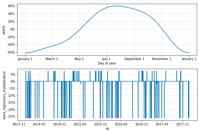
Figure 8.3 – Cropped components plot of binary additional regressors

The trend, weekly seasonality, and yearly seasonality, which were cropped out, look much the same as we've seen before with this dataset. However, we have a new addition to the components plot, called extra_regressors_multiplicative. Had we specified some of those regressors as additive, we would see a second subplot here, called extra_regressors_additive.

On dates where the value is at 0%, these are our baseline dates when the weather was cloudy, which we left out of the additional regressors. The other dates are those where the weather deviated from cloudy, which we included. We'll take a more in-depth look at this in a bit. But first, let's bring temperature into our model and add a continuous regressor.

Adding continuous regressors

In this example, we will take everything from the previous example and simply add in one more regressor for temperature. Let's begin by looking at the temperature data:

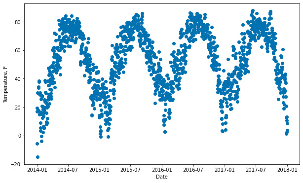
Figure 8.4 – Chicago temperature over time

There's nothing too surprising about the preceding plot; daily temperatures rise in summer and fall in winter. It does look a lot like Figure 4.6 from Chapter 4, Seasonality, but without that increasing trend. Clearly, Divvy ridership and the temperature rise and fall together.

Adding temperature, a continuous variable, is no different than adding binary variables. We simply add another add_regressor call to our Prophet instance, specifying 'temp' for the name, and also including the temperature forecast in our future DataFrame. As we did before, we are fitting our model on the train DataFrame we created, which excludes the final 2 weeks' worth of data. Finally, we plot the components to see what we've got:

model = Prophet(seasonality_mode='multiplicative',

                yearly_seasonality=4)

model.add_regressor('temp')

model.add_regressor('clear')

model.add_regressor('not clear')

model.add_regressor('rain or snow')

model.fit(train)

future = model.make_future_dataframe(periods=14)

future['temp'] = df['temp']

future['clear'] = df['clear']

future['not clear'] = df['not clear']

future['rain or snow'] = df['rain or snow']

forecast = model.predict(future)

fig2 = model.plot_components(forecast)

plt.show()

Now, the extra_regressors_multiplicative plot shows the same fluctuations that our temperature plot displayed:

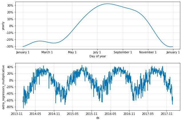
Figure 8.5 – Cropped components plot of both binary and continuous additional regressors

Also note that in Figure 8.2, the yearly plot peaked at 60% effect magnitude. However, now we can see that temperature accounts for some of that effect. The yearly plot in Figure 8.4 shows a peak 30% effect, while the extra_regressors_multiplicative plot shows a 40% increase on certain summertime dates and a massive 80% decrease in ridership on certain wintertime dates. To break this down further, we now need to discuss how to interpret this data.

Interpreting the regressor coefficients

Now let's look at how to inspect the effects of these additional regressors. Prophet includes a package called utilities, which has a function that will come in handy here, called regressor_coefficients. Let's import it now:

from fbprophet.utilities import regressor_coefficients

Using it is straightforward. Just pass the model as an argument and it will output a DataFrame with some helpful information about the extra regressors included in the model:

regressor_coefficients(model)

Let's take a look at this DataFrame:

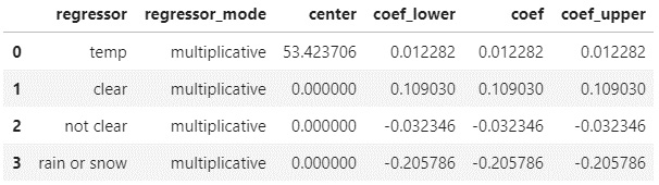
Figure 8.6 – The regressor coefficients DataFrame

It features a row for each extra regressor in your model. In this case, we have one for temperature and three more for the weather conditions we included. The regressor_mode column naturally will have strings of either additive or multiplicative, depending upon the effect of each specific regressor on 'y'. The mean value of the pre-standardized regressor (the raw input data) is saved in the center column. If the regressor wasn't standardized, then the value will be zero.

The coef column is the one you really want to pay attention to. It denotes the expected value of the coefficient. That is, the expected impact on 'y' of a unit increase in the regressor. In the preceding DataFrame, the coef for temp is 0.012282. This coefficient tells us that for every degree higher than the center (53.4, in this case), the expected effect on ridership will be 0.012282, or a 1.2% increase.

For the rain or snow row, which is a binary regressor, it tells us that on those rainy or snowy days, then ridership will be down 20.6% compared to cloudy days, as that was the regressor we left out. Had we included all four weather conditions, to interpret this value, you would say ridership would be down 20.6% compared to the value predicted for the same day if modeled without including weather conditions.

Finally, the columns for 'coef_lower' and 'coef_upper' indicate the lower and upper bounds, respectively, of the uncertainty interval around the coefficient. They are only of interest if mcmc_samples is set to a value greater than zero. Markov chain Monte Carlo samples, or MCMC samples, is a topic you'll learn about in Chapter 10, Uncertainty Intervals. If mcmc_samples is left at the default value, as in these examples, 'coef_lower' and 'coef_upper' will be equal to coef.

Now, to conclude, we can plot each of these extra regressors individually with the plot_forecast_component function we first used in Chapter 5, Holidays. After importing it from Prophet's plot package, we will loop through each regressor in that regressor_coefficients DataFrame to plot it:

from fbprophet.plot import plot_forecast_component

fig, axes = plt.subplots(

                        len(regressor_coefficients(model)),

                        figsize=(10, 15))

for i, regressor in enumerate(

    regressor_coefficients(model)['regressor']):

    plot_forecast_component(model,

                            forecast,

                            regressor,

                            axes[i])

plt.show()

We plotted all of those as subplots in one figure, resulting in the following diagram:

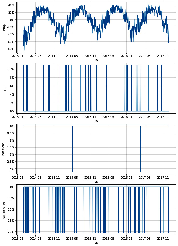
Figure 8.7 – Divvy extra regressor plots

At last, we can visualize the effects of these regressors individually. The magnitudes of these plots should match the coef values in the DataFrame created with the regressor_coefficients function seen in Figure 8.5.

One final note regarding additional regressors in Prophet: they are always modeled as a linear relationship. This means that, for example, our extra regressor of temperature, which was found to increase ridership by 1.2% for every degree increase, is modeling a trend that will continue to infinity. That is, if the temperature were to spike to 120 degrees Fahrenheit, there's no way for us to change the linear relationship and inform Prophet that ridership will probably decrease now that it's getting so hot outside.

Although this is a limitation of Prophet as currently designed, in practice it is not always a great problem. A linear relationship is very often a good proxy for the actual relationship, especially for a small range of data, and will still add a lot of additional information to your model to enrich your forecasts.

Summary

In this chapter, you learned a generalized method to add any additional regressors beyond the holidays, which you learned how to add earlier. You learned that adding both binary regressors, such as weather conditions, and continuous regressors, such as temperature, use the same add_regressor method. You also learned how to use the regressor_coefficients function in Prophet's utilities package to inspect the effects of your additional regressors.

Although you may now want to add all sorts of extra regressors to your forecasts, you also learned that Prophet requires all additional regressors to have defined values going into the future or else there's no information to inform a forecast. This is why we only forecasted 2 weeks out when using weather data.

In the next chapter, we are going to look at how Prophet handles outliers and how you can exert greater control over the process yourself.