Chapter 2: Getting Started with Facebook Prophet

Prophet is an open source piece of software, which means that the entirety of the underlying code is freely available to anyone to inspect and modify. This gives Prophet a great deal of power as any user can add features or fix bugs, but it also has its downsides. Many closed source software packages, such as Microsoft Word or Tableau, come packaged in their own independent installation file with a neat graphical user interface to not only walk users through installation but also enable them to interact with the software once it's installed.

Prophet, in contrast, is accessed through either the Python or R programming languages and depends upon many additional open source libraries. This gives it great flexibility as users can tweak features or even add entirely new ones to suit their specific problem, but it comes with the downside of potentially difficult usability. That's what this book aims to simplify.

In this chapter, we will walk you through the entire installation procedure depending upon which operating system you use, and then together we will build our first forecast by modeling atmospheric carbon dioxide levels over the last few decades.

In full, this chapter will cover the following:

• Installing Prophet
• Building a simple model in Prophet
• Interpreting the forecast DataFrame
• Understanding components plots

Technical requirements

The data files and code for examples in this chapter can be found at https://github.com/PacktPublishing/Forecasting-Time-Series-Data-with-Facebook-Prophet. In this chapter, we will walk through the process of installing many of the requirements. So, to begin this chapter, it is only necessary that you have a Windows, macOS, or Linux machine capable of running Anaconda with Python 3.x.

Installing Prophet

Installing Facebook Prophet on your machine is an easy and straightforward process. However, under the hood, Prophet depends upon the Stan programming language, and installing PyStan, the Python interface for it, is unfortunately not so straightforward because it requires many non-standard compilers.

But don't worry, because there is a really easy way to get Prophet and all dependencies installed, no matter which operating system you use, and that is through Anaconda.

Anaconda is a free distribution of Python that comes bundled with hundreds of additional Python packages that are useful for data science, along with the package management system conda. This is in contrast to installing the Python language from its source on https://www.python.org/, which will include the default Python package manager, called pip.

When pip installs a new package, it will install any dependencies without checking whether these dependent Python packages will conflict with others. This can be a particular problem when one package requires a dependency of one version, while another package requires a different version. You may have, for example, a working installation of Google's TensorFlow package, which requires the NumPy package to work with large, multidimensional arrays, and use pip to install a new package that specifies a different NumPy version as a dependency.

The different version of NumPy would then overwrite the other version and you may find that TensorFlow suddenly doesn't work as expected, or even at all. In contrast, conda will analyze the current environment and work out on its own how to install a compatible set of dependencies for all installed packages and provide a warning if this cannot be done.

PyStan, and many other Python tools, for that matter, require compilers written in the C language. These types of dependencies are unable to be installed using pip, but Anaconda already includes them. Therefore, it is strongly recommended to first install Anaconda.

If you already have a Python environment that you are happy with and do not want to install the full Anaconda distribution, there is a much smaller version available called Miniconda, which only includes conda, Python, and a small number of required packages. Although it is technically possible to install Prophet and all dependencies without Anaconda, it can be extremely difficult and the procedure varies a great deal depending on the machine in use, so writing a single guide to cover all scenarios is nearly impossible.

This guide assumes that you will begin with an Anaconda or Miniconda installation, with Python 3 or greater. If you're unsure of whether you want Anaconda or Miniconda, go with Anaconda. Note that the full Anaconda distribution will require about 3 GB of space on your computer due to all of the packages included, so if space is an issue, you should consider Miniconda instead.

Important note

As of Prophet version 0.6, Python 2 is no longer supported. Be sure that you have Python 3 installed on your machine before proceeding. Installing Anaconda is strongly recommended.

Installation on macOS

If you do not already have Anaconda or Miniconda installed, that should be your first step. Instructions for Anaconda installation can be found in the Anaconda documentation at https://docs.anaconda.com/anaconda/install/mac-os/. If you know that you want Miniconda over Anaconda, start here: https://docs.conda.io/projects/continuumio-conda/en/latest/user-guide/install/macos.html. Use all of the defaults for installation in either case.

With Anaconda or Miniconda installed, installing Prophet can be achieved using conda. Simply run the following two commands in the terminal to first install gcc, a collection of compilers that PyStan requires, and then install Prophet itself, which will automatically also install PyStan:

conda install gcc

conda install -c conda-forge fbprophet

And after that, you should be able to get started! You can skip ahead to the next section where we see how to build your first model.

Installation on Windows

As with macOS, the first step is to ensure that Anaconda or Miniconda is installed. Anaconda installation instructions can be found at https://docs.anaconda.com/anaconda/install/windows/, and those for Miniconda are available here: https://docs.conda.io/projects/continuumio-conda/en/latest/user-guide/install/windows.html.

On Windows, you must check the box to register Anaconda as the default Python. This is required to get PyStan installed correctly. You may see a different version of Python, such as Python 3.8, than shown here:

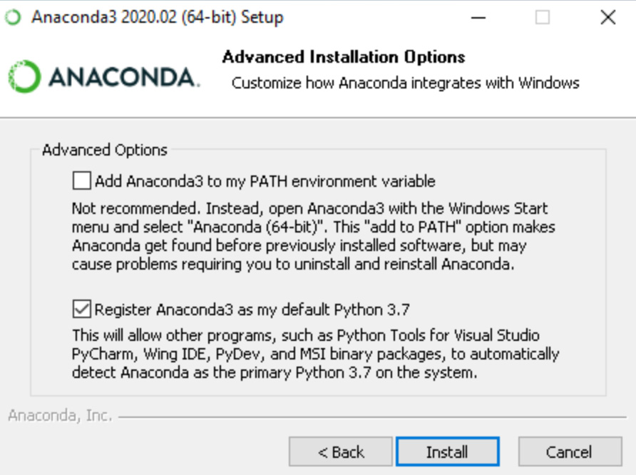
Figure 2.1 – Registering Anaconda as the default Python

Once Anaconda or Miniconda is installed, you'll have access to the conda package manager, which greatly simplifies Prophet's installation on Windows by getting around many issues with PyStan installation. First, install gcc, which is a collection of compilers that PyStan requires, and then install Prophet itself, which will automatically also install PyStan, by running the following two commands in your Command Prompt:

conda install gcc

conda install -c conda-forge fbprophet

That second command includes additional syntax to instruct conda to look at the conda-forge channel for the Facebook Prophet files. conda-forge is a community effort that allows developers to provide their software as a conda package. Prophet is not included in the default Anaconda distribution, but with the conda-forge channel, and the Facebook team can provide access directly through conda.

That should leave you with Prophet successfully installed!

Installation on Linux

Installing Anaconda on Linux requires just a few additional steps compared with macOS or Windows, but they should not pose any problems. Full instructions can be found in Anaconda's documentation at https://docs.anaconda.com/anaconda/install/linux/. Instructions for Miniconda are available at https://docs.conda.io/projects/continuumio-conda/en/latest/user-guide/install/linux.html.

Because Linux is offered by various distributions, it is not possible to write a fully comprehensive guide for Prophet installation. However, if you are already using Linux, it is a fair assumption that you are also well versed in its intricacies.

Just make sure that you have the gcc, g++, and build-essential compilers installed and the python-dev and python3-dev Python development tools. If your Linux distribution is a Red Hat system, install gcc64 and gcc64-c++. After that, use conda to install Prophet:

conda install -c conda-forge fbprophet

If everything went well, you should be ready to go now! Let's test it out by building your first model.

Building a simple model in Prophet

The longest record of direct measurements of CO2 in the atmosphere was started in March 1958 by Charles David Keeling of the Scripps Institution of Oceanography. Keeling was based in La Jolla, California, but had received permission from the National Oceanic and Atmospheric Administration (NOAA) to use their facility located two miles above sea level on the northern slope of Mauna Loa, a volcano on the island of Hawaii, to collect carbon dioxide samples. At that elevation, Keeling's measurements would be unaffected by local releases of CO2, such as from nearby factories.

In 1961, Keeling published the data he had collected thus far, establishing that there was strong seasonal variation in CO2 levels and that they were rising steadily, a trend that later became known as the Keeling Curve. By May 1974, the NOAA had begun their own parallel measurements and have continued since then. The Keeling Curve graph is as follows:

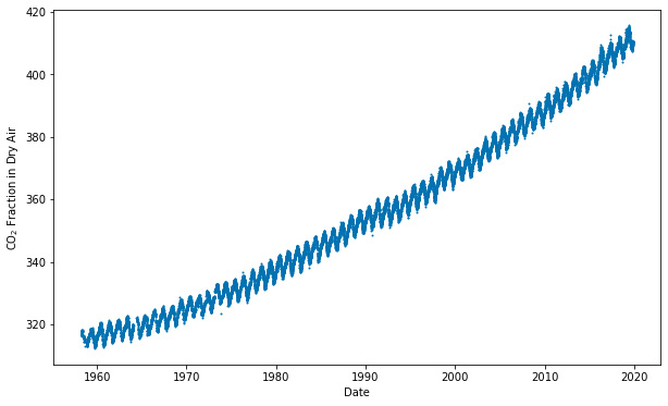
Figure 2.2 – The Keeling Curve, showing the concentration of carbon dioxide in the atmosphere

With its seasonality and increasing trend, this curve is a good candidate to try out Prophet. This dataset contains over 19,000 daily observations across 53 years. The unit of measurement for CO2 is PPM, or parts per million, a measure of CO2 molecules per million molecules of air.

To begin our model, we need to import the necessary libraries, pandas and Matplotlib, and import the Prophet class from the fbprophet package:

import pandas as pd

import matplotlib.pyplot as plt

from fbprophet import Prophet

As input, Prophet always requires a pandas DataFrame with two columns:

• ds, for datestamp, should be a datestamp or timestamp column in a format expected by pandas.
• y, a numeric column containing the measurement we wish to forecast.

Here, we use pandas to import the data, in this case a csv file, and then load it into a DataFrame. Note that we also convert the ds column to a pandas datetime format, to ensure that pandas is correctly identifying it as dates and not simply loading it as an alphanumeric string:

df = pd.read_csv('co2-ppm-daily_csv.csv')

df['date'] = pd.to_datetime(df['date'])

df.columns = ['ds', 'y']

If you're familiar with the scikit-learn (sklearn) package, you'll feel right at home in Prophet because it was designed to operate in a similar way. Prophet follows the sklearn paradigm of first creating an instance of the model class before calling the fit and predict methods:

model = Prophet()

model.fit(df)

In that single fit command, Prophet analyzed the data and isolated both the seasonality and trend without requiring us to specify any additional parameters. It has not yet made any future forecast, though. To do that, we need to first make a DataFrame of future dates and then call the predict method. The make_future_dataframe method requires us to specify the number of days we intend to forecast out. In this case, we will choose 10 years, or 365 days, times 10:

future = model.make_future_dataframe(periods=365 * 10)

forecast = model.predict(future)

At this point, the forecast DataFrame contains Prophet's prediction for CO2 concentrations going 10 years into the future. We will explore that DataFrame in a moment, but first let's plot the data using Prophet's plot functionality. The plot method is built upon Matplotlib; it requires a DataFrame output from the predict method (our forecast DataFrame in this example).

We're labeling the axes with the optional xlabel and ylabel arguments, but just sticking with the default for the optional figsize argument. Note that I am also adding a title using raw Matplotlib syntax; because the Prophet plot is built upon Matplotlib, anything you can do to a Matplotlib figure can be performed here as well. Also, don't be confused by the odd ylabel text with the dollar signs; that just tells Matplotlib to use its own TeX-like engine to make the subscript in CO2:

fig = model.plot(forecast, xlabel='Date',

                 ylabel=r'CO$_2$ PPM')

plt.title('Daily Carbon Dioxide Levels Measured at Mauna Loa')

plt.show()

The graph is as follows:

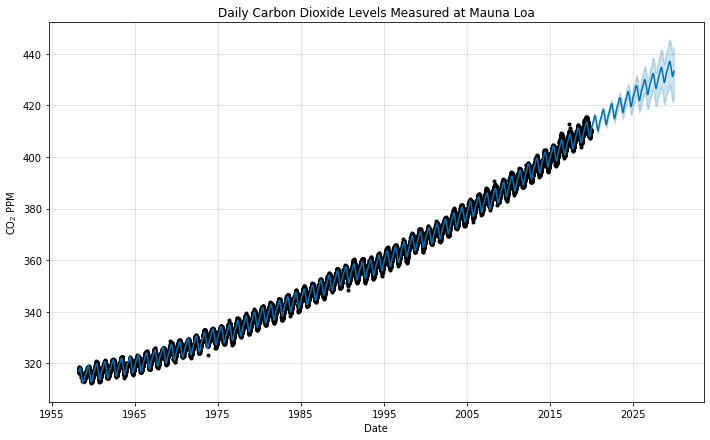
Figure 2.3 – Prophet forecast

And that's it! In those 12 lines of code, we have arrived at our 10-year forecast.

Interpreting the forecast DataFrame

Now, let's take a look at that forecast DataFrame by displaying the first three rows (I've transposed it here, in order to better see the column names on the page) and learn how these values were used in the preceding chart:

forecast.head(3).T

After running that command, you should see the following table print out:

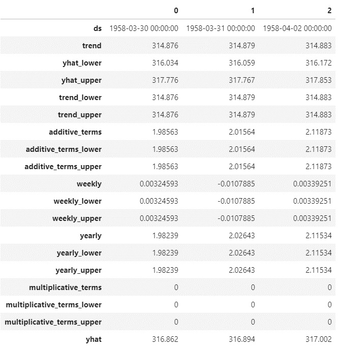
Figure 2.4 – The forecast DataFrame

The following is a description of each of the columns in the forecast DataFrame:

• 'ds': Datestamp or timestamp that values in that row pertain to
• 'trend': Value of the trend component alone
• 'yhat_lower': Lower bound of the uncertainty interval around the final prediction
• 'yhat_upper': Upper bound of the uncertainty interval around the final prediction
• 'trend_lower': Lower bound of the uncertainty interval around the trend component
• 'trend_upper': Upper bound of the uncertainty interval around the trend component
• 'additive_terms': Combined value of all the additive seasonalities
• 'additive_terms_lower': Lower bound of the uncertainty interval around the additive seasonalities
• 'additive_terms_upper': Upper bound of the uncertainty interval around the additive seasonalities
• 'weekly': Value of the weekly seasonality component
• 'weekly_lower': Lower bound of the uncertainty interval around the weekly component
• 'weekly_upper': Upper bound of the uncertainty interval around the weekly component
• 'yearly': Value of the yearly seasonality component
• 'yearly_lower': Lower bound of the uncertainty interval around the yearly component
• 'yearly_upper': Upper bound of the uncertainty interval around the yearly component
• 'multiplicative_terms': Combined value of all the multiplicative seasonalities
• 'multiplicative_terms_lower': Lower bound of the uncertainty interval around the multiplicative seasonalities
• 'multiplicative_terms_upper': Upper bound of the uncertainty interval around the multiplicative seasonalities
• 'yhat': Final predicted value; a combination of 'trend', 'multiplicative_terms', and 'additive_terms'

If the data contains a daily seasonality, then columns for 'daily', 'daily_upper', and 'daily_lower' will also be included, following the pattern established with the 'weekly' and 'yearly' columns. Later chapters will include discussion and examples of both the additive/multiplicative seasonalities and of the uncertainty intervals.

Tip

yhat is pronounced as why hat. It comes from the statistical notation where the variable ŷ represents a predicted value of the variable y. In general, placing a hat, or caret, over a true parameter denotes an estimator of it.

In Figure 2.3, the black dots represent the actual recorded y values we fit on (those in the df['y'] column), whereas the solid line represents the calculated yhat values (the forecast['yhat'] column). Note that the solid line extends beyond the range of the black dots where we have forecasted into the future. The lighter shading notable around the solid line in the forecasted region represents the uncertainty interval, bound by forecast['yhat_lower'] and forecast['yhat_upper'].

Now let's break down that forecast into its components.

Understanding components plots

In Chapter 1, The History and Development of Time Series Forecasting, Prophet was introduced as an additive regression model. Figures 1.4 and 1.5 showed how individual component curves for the trend and the different seasonalities are added together to create a more complex curve. The Prophet algorithm essentially does this in reverse; it takes a complex curve and decomposes it into its constituent parts. The first step toward greater control of a Prophet forecast is to understand these components so that they can be manipulated individually. Prophet provides a plot_components method to visualize these.

Continuing on with our progress on the Mauna Loa model, plotting the components is as simple as running these commands:

fig2 = model.plot_components(forecast)

plt.show()

As you can see in the output plot, Prophet has isolated three components in this dataset: trend, weekly seasonality, and yearly seasonality:

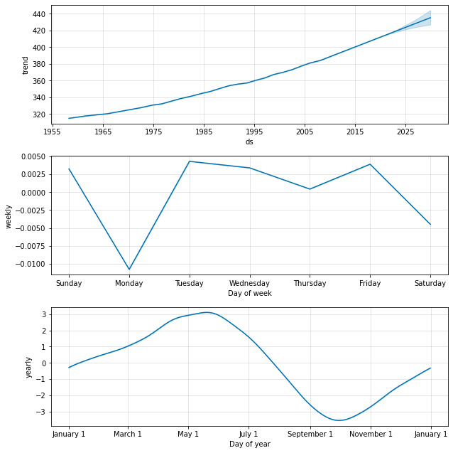
Figure 2.5 – Mauna Loa components plot

The trend constantly increases but seems to have a steepening slope as time progresses—an acceleration of CO2 concentration in the atmosphere. The trend line also shows slim uncertainty intervals in the forecasted year. From this curve, we learn that atmospheric CO2 concentrations were about 320 ppm in 1965. This grew to about 400 by 2015 and we expect about 430 PPM by 2030. However, these exact numbers will vary depending upon the day of the week and the time of year, due to the existence of the seasonality effects.

The weekly seasonality shows that by days of the week, values will vary by about 0.01 PPM—an insignificant amount and most likely due purely to noise and random chance. Indeed, intuition tells us that carbon dioxide levels (when measured far enough away from human activity, as they are on the high slopes of Mauna Loa) do not care much what day of the week it is and are unaffected by it.

We will learn in Chapter 4, Seasonality, how to instruct Prophet not to fit a weekly seasonality, as is prudent in this case. In Chapter 10, Uncertainty Intervals, we will learn how to plot uncertainty for seasonality and ensure that a seasonality such as this can be ignored.

Now, looking at the yearly seasonality reveals that carbon dioxide rises throughout the winter and peaks in May or so, while falling in the summer with a trough in October. Measurements of carbon dioxide can be 3 PPM above or 3 PPM below what the trend alone would predict, based upon the time of year. If you refer back to the original data, plotted in Figure 2.2, you will be reminded that there was a very obvious cyclical nature to the curve, captured with this yearly seasonality.

As simple as that model was, that is often all you need to make very accurate forecasts with Prophet! We used no additional parameters than the defaults and yet achieved very good results.

Summary

Hopefully, you experienced no issues installing Prophet on your machine at the beginning of this chapter. The potential challenge of getting the Stan dependency installed is greatly eased by using the Anaconda distribution of Python. After installation, we looked at the carbon dioxide levels measured in the atmosphere two miles above the Pacific Ocean, at Mauna Loa in Hawaii. We built our first Prophet model and, in just 12 lines of code, were able to forecast the next 10 years of carbon dioxide levels.

After that, we inspected the forecast DataFrame and saw the rich results that Prophet outputs. Finally, we plotted the components of the forecast - the trend, yearly seasonality, and weekly seasonality, to better understand the data's behavior.

There is a lot more to Prophet than just this simple example, though. The remainder of this book will be spent demonstrating all of the parameters and additional features available that allow you to have greater control over your forecasts. Next, we'll take a look at non-daily data to see what precautions and adjustments need to be taken, thereby preparing us to handle datasets with different time granularities.