7
Test Adequacy Assessment Using Control Flow and Data Flow
CONTENTS
7.2 Adequacy criteria based on control flow
7.4 Adequacy criteria based on data flow
7.5 Control flow versus data flow
7.7 Structural and functional testing
This chapter introduces methods for the assessment of test adequacy and test enhancement. Measurements of test adequacy using criteria based on control flow and data flow are explained. These code based coverage criteria allow a tester to determine how much of the code has been tested and what remains untested.
7.1 Test Adequacy: Basics
7.1.1 What is test adequacy?
Consider a program P written to meet a set R of functional requirements. We notate such a P and R as (P, R). Let R contain n requirements labeled R1, R2, . . . , Rn. Suppose now that a set Τ containing k tests has been constructed to test P to determine whether or not it meets all the requirements in R. Also, P has been executed against each test in Τ and has produced correct behavior. We now ask: Is Τ good enough? This question can be stated differently as: Has P been tested thoroughly? or as: Is Τ adequate? Regardless of how the question is stated, it assumes importance when one wants to test P thoroughly in the hope that all errors have been discovered and removed when testing is declared complete and the program P declared usable by the intended users.
Test adequacy refers to the “goodness” of a test set. The “goodness” ought to be measured against a quantitative criterion.
In the context of software testing, the terms “thorough,” “good enough,”and “adequate,” used in the questions above, have the same meaning. We prefer the term “adequate” and the question Is Τ adequate? Adequacy is measured for a given test set designed to test Ρ to determine whether or not Ρ meets its requirements. This measurement is done against a given criterion C. A test set is considered adequate with respect to criterion C when it satisfies C. The determination of whether or not a test set T for program P satisfies criterion C depends on the criterion itself and is explained later in this chapter.
Functional requirements are concerned with application functionality. Non-functional requirements include characteristics such as performance, reliability, usability.
In this chapter we focus only on functional requirements, testing techniques to validate non-functional requirements are dealt with elsewhere.
Example 7.1 Consider the problem of writing a program named sumProduct that meets the following requirements:
R1: Input two integers, say x and y, from the standard input device.
R2.1: Find and print to the standard output device the sum of x and y if x < y.
R2.2: Find and print to the standard output device the product of x and y if x ≥ y.
Suppose now that the test adequacy criterion C is specified as follows:
C: A test Τ for program (P,R) is considered adequate if for each requirement r in R there is at least one test case in Τ that tests the correctness of Ρ with respect to r.
It is obvious that Τ = {t :< x = 2, y = 3 >} is inadequate with respect to C for program sumProduct. The only test case t in Τ tests R1 and R2.1., but not R2.2.
7.1.2 Measurement of test adequacy
Adequacy of a test set is measured against a finite set of elements. Depending on the adequacy criterion of interest, these elements are derived from the requirements or from the program under test. For each adequacy criterion C, we derive a finite set known as the coverage domain and denoted as Ce.
Test adequacy is measured against a coverage domain. Such a domain could be based on requirements or elements of the code. A test set that is adequate only with respect to a requirements based coverage domain is likely to be weaker than that adequate with respect to both requirements and code-based coverage domains.
A criterion C is a white-box test adequacy criterion if the corresponding coverage domain Ce depends solely on program Ρ under test. A criterion C is a black-box test adequacy criterion if the corresponding coverage domain Ce depends solely on requirements R for the program Ρ under test. All other test adequacy criteria are of a mixed nature and not considered in this chapter. This chapter introduces several white-box test adequacy criteria that are based on the flow of control and the flow of data within the program under test.
An adequacy criterion derived solely from a code-based coverage domain is a white-box criterion. That derived from a requirements-based coverage domain is a black box. criterion.
Suppose that it is desired to measure the adequacy of T. Given that Ce has n ≥ 0 elements, we say that Τ covers Ce if for each element e′ in Ce there is at least one test case in Τ that tests e′. Τ is considered adequate with respect to C if it covers all elements in the coverage domain. Τ is considered inadequate with respect to C if it covers k elements of Ce where k < n. The fraction k/n is a measure of the extent to which Τ is adequate with respect to C. This fraction is also known as the coverage of Τ with respect to C, P, and R.
The determination of when an element e is considered tested by Τ depends on e and Ρ and is explained below through examples.
Example 7.2 Consider the program P, test T, and adequacy criterion C of Example 7.1. In this case the finite set of elements Ce is the set {R1, R2.1, R2.2}. Τ covers R1 and R2.l but not R2.2. Hence Τ is not adequate with respect to C. The coverage of Τ with respect to C, P, and R is 0.66. Element R2.2 is not tested by Τ whereas the other elements of Ce are tested.
Example 7.3 Next let us consider a different test adequacy criterion which is referred to as the path coverage criterion.
C: A test Τ for program (P,R) is considered adequate if each path in P is traversed at least once.
Given the requirements in Example 7.1 let us assume that Ρ has exactly two paths, one corresponding to condition x < y and the other to x ≥ y. Let us refer to these two paths as p1 and p2, respectively. For the given adequacy criterion C we obtain the coverage domain Ce to be the set {p1,p2}.
To measure the adequacy of Τ of Example 7.1 against C, we execute Ρ against each test case in Τ. As Τ contains only one test for which x <y, only the path p1 is executed. Thus the coverage of Τ with respect to C, P, and R is 0.5 and hence Τ is not adequate with respect to C. We also say that p2 is not tested.
In Example 7.3, we assumed that Ρ contains exactly two paths. This assumption is based on a knowledge of the requirements. However, when the coverage domain must contain elements from the code, these elements must be derived by program analysis and not by an examination of its requirements. Errors in the program and incomplete or incorrect requirements might cause the program, and hence the coverage domain, to be different from what one might expect.
A code-based coverage domain is derived through the analysis of the program under test.
Example 7.4 Consider the following program written to meet the requirements specified in Example 7.1; the program is obviously incorrect.
Program P7.1
1 begin
2 int x, y;
3 input (x, y);
4 sum=x+y;
5 output (sum);
6 end
The above program has exactly one path which we denote as p1. This path traverses all statements. Thus, to evaluate any test with respect to criterion C of Example 7.3, we obtain the coverage domain Ce to be {p1}. It is easy to see that Ce is covered when Ρ is executed against the sole test in Τ of Example 7.1. Thus Τ is adequate with respect to Ρ even though the program is incorrect.
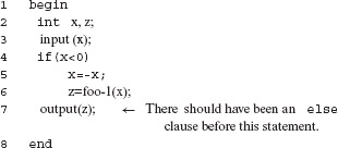
Program P7.1 has an error that is often referred to as a “missing path” or a “missing condition” error. A correct program that meets the requirements of Example 7.1 follows.
1 begin
2 int x, y;
3 input (x, y);
4 if(x<y)
5 then
6 output (x+y);
7 else
8 output (x*y);
9 end
A missing condition leads to a missing path error. There is no guarantee that such an error will be detected by a test set adequate with respect to any white box or black box criteria that has a finite coverage domain.
This program has two paths, one of which is traversed when x < y and the other when x≥y. Denoting these two paths by p1 and p2 we obtain the coverage domain given in Example 7.3. As mentioned earlier, test Τ of Example 7.1 is not adequate with respect to the path coverage criterion.
The above example illustrates that an adequate test set might not reveal even the most obvious error in a program. This does not diminish in any way the need for the measurement of test adequacy. The next section explains the use of adequacy measurement as a tool for test enhancement.
7.1.3 Test enhancement using measurements of adequacy
While a test set adequate with respect to some criterion does not guarantee an error-free program, an inadequate test set is a cause for worry. Inadequacy with respect to any criterion often implies deficiency. Identification of this deficiency helps in the enhancement of the inadequate test set. Enhancement in turn is also likely to test the program in ways it has not been tested before such as testing untested portion, or testing the features in a sequence different from the one used previously. Testing the program differently than before raises the possibility of discovering any uncovered errors.
Quantitatively measured inadequacy of a test set is an opportunity for its enhancement.
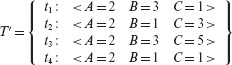
Example 7.5 Let us reexamine test Τ for P7.2 in Example 7.4. To make Τ adequate with respect to the path coverage criterion, we need to add a test that covers p2. One test that does so is {< x = 3, y = 1 >}. Adding this test to Τ and denoting the expanded test set by T′, we get
T′ = {< x = 2, y = 3 >, < x = 3, y = 1 >}.
When P7.2 is excuted against the two tests in T′ , both paths p1 and p2 are traversed. Thus T′ is adequate with respect to the path coverage criterion.
Given a test set Τ for program P, test enhancement is a process that depends on the test process employed in the organization. For each new test added to Τ, Ρ needs to be executed to determine its behavior. An erroneous behavior implies the existence of an error in Ρ and will likely lead to debugging of Ρ and the eventual removal of the error. However, there are several procedures by which the enhancement could be carried out. One such procedure follows.
Procedure for Test Enhancement Using Measurements of Test Adequacy.
Step 1
Measure the adequacy of T with respect to the given criterion C. If T is adequate then go to Step 3, otherwise execute the next step. Note that during adequacy measurement we will be able to determine the uncovered elements of Ce.
Step 2
For each uncovered element e ∈ Ce, do the following until e is covered or is determined to be infeasible.
2.1
Construct a test t that covers e or will likely cover e.
2.2
Execute P against t.
2.2.1
If P behaves incorrectly then we have discovered the existence of an error in P. In this case t is added to T, the error is removed from P and this procedure gets repeated from the beginning.
2.2.2
If P behaves correctly and e is covered then t is added to T, otherwise it is the tester’s option whether to ignore t or to add it to T.
Step 3
Test enhancement is complete.
End of procedure
Adequacy-based test enhancement is a cycle in which a test set is enhanced by an examination of which parts of the corresponding coverage domain are not covered. New tests added are designed to cover the uncovered portions of the coverage domain and thus enhance the test set.
Figure 7.1 shows a sample test construction-enhancement cycle. The cycle begins with the construction of a non-empty set Τ of test cases. These tests cases are constructed from the requirements of program Ρ under test. Ρ is then executed against all test cases. If Ρ fails on one or more of the test cases then it ought to be corrected by first finding and then removing the source of the failure. The adequacy of Τ is measured with respect to a suitably selected adequacy criterion C after Ρ is found to behave satisfactorily on all elements of T. This construction-enhancement cycle is considered complete if Τ is found adequate with respect to C. If not, then additional test cases are constructed in an attempt to remove the deficiency.
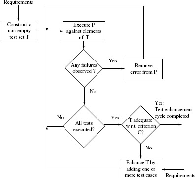
Figure 7.1 A test construction-enhancement cycle.
The construction of these additional test cases once again makes use of the requirements that Ρ must meet.
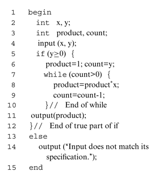
Example 7.6 Consider the following program intended to compute xy given integers x and y. For y < 0 the program skips the computation and outputs a suitable error message.
Program P7.3
Next, consider the following test adequacy criterion.
C: A test Τ is considered adequate if it tests P7.2 for at least one zero and one non-zero value of each of the two inputs x and y.
The coverage domain for C can be determined using C alone and without any inspection of P7.3. For C, we get Ce = {x = 0, y = 0, x ≠ 0, y ≠ 0}. Again, one can derive an adequate test set for 7.6 by a simple examination of Ce. One such test set is
T = {< x = 0, y = 1 >, < x = 1, y = 0 >}.
In this case, we need not apply the enhancement procedure given above. Of course, P7.3 needs to be executed against each test case in Τ to determine its behavior. For both tests it generates the correct output which is 0 for the first test case and 1 for the second. Note that Τ might well be generated without reference to any adequacy criterion.
Example 7.7 Criterion C of Example 7.6 is a black-box coverage criterion as it does not require an examination of the program under test for the measurement of adequacy. Let us consider the path coverage criterion defined in Example 7.3. An examination of P7.3 reveals that it has an indeterminate number of paths due to the presence of a while loop. The number of paths depends on the value of y and hence that of count. Given that y is any non-negative integer, the number of paths can be arbitrarily large. This simple analysis of paths in P7.3 reveals that we cannot determine the coverage domain for the path coverage criterion.
A black-box coverage criterion does not require an examination of the program under test in order to generate new tests.
The usual approach in such cases is to simplify C and reformulate it as follows.
C: A test Τ is considered adequate if it tests all paths. In case the program contains a loop, then it is adequate to traverse the loop body zero times and once.
The modified path coverage criterion leads to
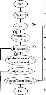
= {p1, p2, p3}. The elements of Ce are enumerated below with respect to Figure 7.2.
Figure 7.2 Control flow graph of P7.6.
p1: [1→2→3→4→5→7→9]; corresponds to y ≥ 0 and loop body traversed zero times.
p2: [1→2→3→4→5→6→5→7→9]; corresponds to y ≥ 0 and loop body traversed once.
p3: [1→2→3→8→9]; corresponds to y < 0 and the control reaches the output statement without entering the body of the while loop.
A possible coverage domain consists of all paths in a program. Such a domain is made finite by assuming that each loop body in the program is skipped on at least one arrival at the loop and it is executed at least once on another arrival.
The coverage domain for C′ and P7.3 is {p1, p2, p3}. Following the test enhancement procedure, we first measure the adeqacy of Τ with respect to C′. This is done by executing P against each element of Τ and determining which elements in
Moving on to Step 2, we attempt to construct a test aimed at covering p3. Any test case with y < 0 will cause p3 to be traversed.
Let us use the test case t :< x = 5, y = –1 >. When P is executed against t, indeed path p3 is covered and P behaves correctly. We now add t to Τ. The loop in Step 2 is now terminated as we have covered all feasible elements of
Note that Τ is adequate with respect to C′, but is Program P7.3 correct?
7.1.4 Infeasibility and test adequacy
An element of the coverage domain is infeasible if it cannot be covered by any test in the input domain of the program under test. In general, it is not possible to write an algorithm that would analyze a given program and determine if a given element in the coverage domain is feasible or not. Thus it is usually the tester who determines whether or not an element of the coverage domain is infeasible.
An element of a coverage domain, e.g., a path, might be infeasible to cover. This implies that there exists no test case that covers such an element.
Feasibility can be demonstrated by executing the program under test against a test case and showing that indeed the element under consideration is covered. However, infeasibility cannot be demonstrated by program execution against a finite number of test cases. Nevertheless, as in Example 7.8, simple arguments can be constructed to show that a given element is infeasible. For more complex programs, the problem of determining infeasibility could be difficult. Thus one might fail while attempting to cover e to enhance a test set by executing P against t.
The conditions that must hold for a test case t to cover an element e of the coverage domain depend on e and P. These conditions are derived later in this chapter when we examine various types of adequacy criteria.
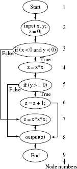
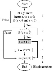
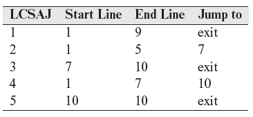
Example 7.8 In this example, we illustrate how an infeasible path occurs in a program. The following program inputs two integers x and y and computes z.
Program P7.4
1 begin
2 int x, y;
3 int z;
4 input (x, y);z=0;
5 if( x<0 and y<0)
6 z=x*x;
7 if (y≥0) z=z+1;
9 else
10 z=x*x*x;
11 output(z);
12 end
The path coverage criterion leads to Ce = {p1,p2,p3}. The elements of Ce are enumerated below with respect to Figure 7.3.
Figure 7.3 Control flow graph of P7.4.
p1: [l → 2 → 3 → 4 → 5 → 6 → 8 → 9]; corresponds to conditions x < 0 and y < 0 and y ≥ 0 evaluating to true.
p2: [l → 2 → 3 → 4 → 5 → 8 → 9]; corresponds to conditions x < 0 and y < 0 evaluating to true and y ≥ 0 to false.
p3: [1 → 2 → 3 → 7 → 8 → 9]; corresponds to x < 0 and y < 0 evaluating to false.
For short programs one might be able to easily categorize a path to be feasible or not. However, for large applications doing so might be a humanly impossible task. The general problem of determining path infeasibility is unsolvable.
It is easy to check that path p1 is infeasible and cannot be traversed by any test case. This is because when control reaches node 5, condition y ≥ 0 is false and hence control can never reach node 6. Thus any test adequate with respect to the path coverage criterion for P7.4 will only cover p2 and p3.
In the presence of one or more infeasible elements in the coverage domain, a test is considered adequate when all feasible elements in the domain have been covered. This also implies that in the presence of infeasible elements, adequacy is achieved when coverage is less than 1.
Infeasible elements in the coverage domain make it harder for testers to generate adequate tests.
Infeasible elements arise for a variety of reasons discussed in subsequent sections. While programmers might not be concerned with infeasible elements, testers attempting to obtain code coverage are. Prior to test enhancement, a tester usually does not know which elements of a coverage domain are infeasible. It is only during an attempt to construct a test case to cover an element that one might realize the infeasibility of an element. For some elements, this realization might come after several failed attempts. This may lead to frustration on the part of the tester. The testing effort spent on attempting to cover an infeasible element might be considered wasteful. Unfortunately there is no automatic way to identify all infeasible elements in a coverage domain derived from an arbitrary program. However, careful analysis of a program usually leads to a quick identification of infeasible elements. We return to the topic of dealing with infeasible elements later in this chapter.
7.1.5 Error detection and test enhancement
The purpose of test enhancement is to determine test cases that test the untested parts of a program. Even the most carefully designed tests based exclusively on requirements can be enhanced. The more complex the set of requirements, the more likely it is that a test set designed using requirements is inadequate with respect to even the simplest of various test adequacy criteria.
Tests designed based only on requirements can often be enhanced significantly by an examination of code that remains untested. Such enhancement has the potential of revealing errors that might have otherwise remained uncovered.
During the enhancement process, one develops a new test case and executes the program against it. Assuming that this test case exercises the program in a way it has not been exercised before, there is a chance that an error present in the newly tested portion of the program is revealed. In general, one cannot determine how probable or improbable it is to reveal an error through test enhancement. However, a carefully designed and executed test enhancement process is often useful in locating program errors.
Example 7.9 A program to meet the following requirements is to be developed.
R1: Upon start the program offers the following three options to the user:
- Compute xy for integers x and y ≥ 0.
- Compute the factorial of integer x ≥ 0.
- Exit.
R1.1: If the “Compute xy” option is selected then the user is asked to supply the values of x and y, xy is computed and displayed. The user may now select any of the three options once again.
R 1.2: If the “Compute factorial x” option is selected then the user is asked to supply the value of x and factorial of x is computed and displayed. The user may now select any of the three options once again.
R1.3: If the “Exit” option is selected the program displays a goodbye message and exits.
Consider the following program written to meet the above requirements.
Program P7.5
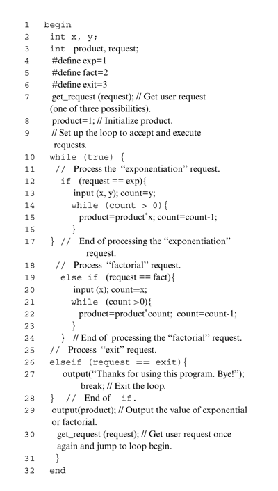
Suppose now that the following set containing three tests labeled t1, t2, and t3 has been developed to test P7.5.
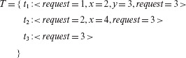
This program is executed against the three tests in the sequence they are listed above. The program is launched once for each input. For the first two of the three requests the program correctly outputs 8 and 24, respectively. The program exits when executed against the last request. This program behavior is correct and hence one might conclude that the program is correct. It will not be difficult for you to believe that this conclusion is incorrect.
A path-based coverage domain consists of all paths in a program such that all loops are executed zero and once. Such executions could be in the same or different runs of the program.
Let us evaluate Τ against the path coverage criterion described earlier in Example 7.9. Before you proceed further, you might want to find a few paths in P7.5 that are not covered by Τ.
The coverage domain consists of all paths that traverse each of the three loops zero and once in the same or different executions of the program. We leave the enumeration of all such paths in P7.5 as an exercise. For this example, let us consider the path that begins execution at line 1, reaches the outermost while at line 10, then the first if at line 12, followed by the statements that compute the factorial starting at line 20, and then the code to compute the exponential starting at line 13. For this example, we do not care what happens after the exponential has been computed and output.
Our tricky path is traversed when the program is launched and the first input request is to compute the factorial of a number, followed by a request to compute the exponential. It is easy to verify that the sequence of requests in Τ do not exercise p. Therefore Τ is inadequate with respect to the path coverage criterion.
To cover p we construct the following test:
When the values in T′ are input to our example program in the sequence given, the program correctly outputs 24 as the factorial of 4 but incorrectly outputs 192 as the value of 23. This happens because T′ traverses our tricky path which makes the computation of the exponentiation begin without initializing product. In fact the code at line 14 begins with the value of product set to 24.
Note that in our effort to increase the path coverage we constructed T′. Execution of the test program on T′ did cover a path that was not covered earlier and revealed an error in the program.
7.1.6 Single and multiple executions
In Example 7.9, we constructed two test sets Τ and T′. Notice that both Τ and T′ contain three tests one for each value of variable request. Should Τ be considered a single test or a set of three tests? The same question applies also to T′. The answer depends on how the values in Τ are input to the test program. In our example, we assumed that all three tests, one for each value of request, are input in a sequence during a single execution of the test program. Hence we consider T as a test set containing one test case and write it as follows:
An test sequence input in one run of the program might not reveal an error that could otherwise be revealed when the same test is input across multiple runs. Of course, this assume that the test can be partitioned so that individual portions are input across different runs. Note that each run starts the program fro its initial state.
Note the use of the outermost angular brackets to group all values in a test. Also, the right arrow (→) indicates that the values of variables are changing in the same execution. We can now rewrite T′ also in a way similar to Τ. Combining Τ and T′, we get a set T′′ containing two test cases written as follows:
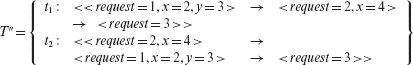
Test set T′′ contains two test cases, one that came from Τ and the other from T′. You might wonder why so much fuss regarding whether something is a test case or a test set. In practice, it does not matter. Thus you may consider T as a set of three test cases or simply as a set of one test case. However, we do want to stress the point that distinct values of all program inputs may be input in separate runs or in the same run of a program. Hence a set of test cases might be input in a single run or in separate runs.
In older programs that were not based on Graphical User Interfaces (GUI), it is likely that all test cases were executed in separate runs. For example, while testing a program to sort an array of numbers, a tester usually executed the sort program with different values of the array in each run. However, if the same sort program is “modernized” and a GUI added for ease of use and marketability, one may test the program with different arrays input in the same run.
Programs that offer a GUI for user interaction are likely to be tested across multiple test cases in a single run.
In the next section, we introduce various criteria based on the flow of control for the assessment of test adequacy. These criteria are applicable to any program written in a procedural language such as C. The criteria can also be used to measure test adequacy for programs written in object oriented languages such as Java and C++. Such criteria include plain method coverage as well as method coverage within context. The criteria presented in this chapter can also be applied to programs written in low level languages such as an assembly language. We begin by introducing control flow based test adequacy criteria.
7.2 Adequacy Criteria Based on Control Flow
7.2.1 Statement and block coverage
Any program written in a procedural language consists of a sequence of statements. Some of these statements are declarative, such as the #define and int statements in C, while others are executable, such as the assignment, if and while statements in C and Java. Note that a statement such as
if count=10;
could be considered declarative because it declares the variable count to be an integer. This statement could also be considered as executable because it assigns 10 to the variable count. It is for this reason that in C we consider all declarations as executable statements when defining test adequacy criteria based on the flow of control.
Programs in a procedural language consists of a set of functions, each function being a sequence of statements. In OO languages the programs are structured into classes where each class often contains multiple methods (functions).
Recall from Chapter 1 that a basic block is a sequence of consecutive statements that has exactly one entry point and one exit point. For any procedural language, adequacy with respect to the statement coverage and block coverage criteria are defined as follows.
Statement Coverage:
The statement coverage of Τ with respect to (P,R) is computed as |Sc|/(|Se| − |Si|), where Sc is the set of statements covered, Si the set of unreachable statements, and Se is the coverage domain consisting of the set of statements in the program. Τ is considered adequate with respect to the statement coverage criterion if the statement coverage of Τ with respect to (P,R) is 1.
Block Coverage:
The block coverage of Τ with respect to (P,R) is computed as |Bc|/(|Be| – |Bi |), where Bc is the set of blocks covered, Bi the set of unreachable blocks, and Be the blocks in the program, i.e. the block coverage domain. Τ is considered adequate with respect to the block coverage criterion if the block coverage of Τ with respect to (P,R) is 1.
In the above definitions, the coverage domain for statement coverage is the set of all statements in the program under test. Similarly, the coverage domain for block coverage is the set of all basic blocks in the program under test. Note that we use the term “unreachable” to refer to statements and blocks that fall on an infeasible path.
A rather simple test adequacy criterion is based on statement coverage. In this case the coverage domain consists of all statements in the program under test. Alternately, the coverage domain could also be a set of basic blocks in the program under test.
The next two examples explain the use of the statement and block coverage criteria. In these examples we use line numbers in a program to refer to a statement. For example, the number 3 in Se for 7.1.2 refers to the statement on line 3 of this program, i.e. to the input (x, y) statement. We will refer to blocks by block numbers derived from the flow graph of the program under consideration.
Example 7.10 The coverage domain corresponding to statement coverage for P7.4 is given below.
Se = {2, 3, 4, 5, 6, 7, 7b, 9, 10}
Here we denote the statement z = z + 1; as 7b. Consider a test set T1 that consists of two test cases against which P7.4 has been executed.
T1 = {t1:<x = – 1, y = – 1 >, t2:< x = 1, y =1 >}
Statements 2, 3, 4, 5, 6, 7, and 10 are covered upon the execution of P against t1. Similarly, the execution against t2 covers statements 2, 3, 4, 5, 9, and 10. Neither of the two tests covers statement 7b which is unreachable as we can conclude from Example 7.8. Thus we obtain |Sc| = 8, |Si| = 1, |Se| = 9. The statement coverage for Τ is 8/(9 – 1) = 1. Hence we conclude that Τ is adequate for (P, R) with respect to the statement coverage criterion.
Example 7.11 The five blocks in P7.4 are shown in Figure 7.4. The coverage domain for the block coverage criterion Be = {1, 2, 3, 4, 5}. Consider now a test set T2 containing three tests against which P7.4 has been executed.
Figure 7.4 Control flow graph of 7.8. Blocks are numbered 1 through 5. The shaded block 3 is infeasible because the condition in block 2 will never be true.
Some blocks in a coverage domain might be infeasible. Such infeasibility is usually discovered manually.
Blocks 1, 2, and 5 are covered when the program is executed against test t1. Tests t2 and t3 also execute exactly the same set of blocks. For T2 and P7.4, we obtain |Be| = 5, |Bc| = 3, and |Bi| = 1. The block coverage can now be computed as 3/(5 – 1) = 0.75. As the block coverage is less than 1, T2 is not adequate with respect to the block coverage criterion.
Coverage values are generally computed as a ratio of the number of items covered to the number of feasible items in the coverage domain. Hence, this ratio is between 0 and 1. It is rare to find a ratio of 1, i.e. 100% statement coverage when testing large and complex applications.
It is easy to check that the test set of Example 7.10 is indeed adequate with respect to the block coverage criterion. Also, T2 can be made adequate with respect to the block coverage criterion by the addition of test t2 from T1 in the previous example.
The formulae given in this chapter for computing various types of code coverage yield a coverage value between 0 and 1. However, while specifying a coverage value, one might instead use percentages. For example, a statement coverage of 0.65 is the same as 65% statement coverage.
7.2.2 Conditions and decisions
To understand the remaining adequacy measures based on control flow, we need to know what exactly constitutes a condition and a decision. Any expression that evaluates to true or false constitutes a condition. Such an expression is also known as a predicate. Given that A, B, and D are Boolean variables, and x and y are integers, A, x > y, A or B, A and (x<y), (A and B) or (A and D) and (¬ D), (A xor B) and (x ≥ y), are all conditions. In these examples, and, or, xor, and ¬ are known as Boolean, or logical, operators. Note that in programming language C, x and x+y are valid conditions, and the constants 1 and 0 correspond to, respectively, true and false.
A simple predicate (or a condition) is made up of a single Boolean variable (possibly with a negation operator) or of a single relational operator. A compound predicate is a concatenation of two or more simple predicates obtained using the Boolean operators AND, OR, and XOR.
Simple and compound conditions: A condition could be simple or compound. A simple condition does not use any Boolean operators except for the ¬ operator. It is made up of variables and at most one relational operator from the set {<, ≤,>,≥, ==, ≠}. A compound condition is made up of two or more simple conditions joined by one or more Boolean operators. In the above examples, A as well as x > y are two simple conditions, while the others are compound. Simple conditions are also referred to as atomic or elementary conditions because they cannot be parsed any further into two or more conditions. Often, the term condition refers to a compound condition. In this book, we will use “condition” to mean any simple or compound condition.
A condition (or a predicate) is used as a decision. The outcome of evaluating a condition is either true or false. A condition involving one or more functions might fail to evaluate in case the function does not terminate appropriately, as for example when it causes the computer to crash.
Conditions as decisions: Any condition can serve as a decision in an appropriate context within a program. As shown in Figure 7.5, most high level languages provide if, while, and switch statements to serve as contexts for decisions. Whereas an if and a while contains exactly one decision, a switch may contain more.
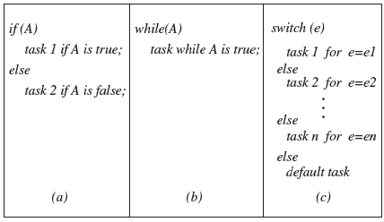
Figure 7.5 Decisions arise in several contexts within a program. Three common contexts for decisions in a C or a Java program are (a) if, (b) while, and (c) switch statements. Note that the if and while statements force the flow of control to be diverted to one of two possible destinations while the switch statement may lead the control to one or more destinations.
A decision can have three possible outcomes, true, false, and undefined. When the condition corresponding to a decision evaluates to true or false, the decision to take one or the other path is taken. In the case of a switch statement, one of several possible paths gets selected and the control flow proceeds accordingly. However, in some cases the evaluation of a condition might fail in which case the corresponding decision’s outcome is undefined.
While a condition used in an if or a looping statement leads the control to follow one of two possible paths, an expression in a switch statement may cause the control to follow one of several paths. A switch statement generally uses expressions that evaluate to a value from a set of multiple values. Of course, it is possible for a switch statement to use a condition. For Fortran programmers, the condition in an if statement may cause the control to select one of three possible paths.
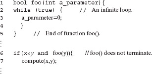
Example 7.12 Consider the following sequence of statements.
Program P7.6
The condition inside the if statement on line 6 will remain undefined because the loop at lines 2–4 will never end. Thus the decision on line 6 evaluates to undefined.
Coupled conditions: There is often the question of how many simple conditions are there in a compound condition. For example, C =(A and B) or (C and A) is a compound condition. Does C contain three or four simple conditions? Both answers are correct depending on one’s point of view. Indeed, there are three distinct conditions A, B, and C. However, the answer is four when one is interested in the number of occurrences of simple conditions in a compound condition. In the example expression above, the first occurrence of A is said to be coupled to its second occurrence.
A condition is considered coupled when it uses a simple predicate more than once.
Conditions within assignments: Conditions may occur within an assignment statement as in the following examples.
- a = x < y; // A simple condition assigned to a Boolean variable a.
- x = p or q; // A compound condition assigned to a Boolean variable x.
- x = y + z * s; if (x)…// Condition true if x = 1, false otherwise.
- a = x < y; x = a * b; // a is used in a subsequent expression for x, but not as a decision.
While predicates are generally used in the context of if and looping statements, most languages allow them to be used on the right side of an assignment statement.
A programmer might want a condition to be evaluated before it is used as a decision in a selection or a loop statement, as in the examples above. Strictly speaking, a condition becomes a decision only when it is used in the appropriate context such as within an if statement. Thus, in the example at line 4, x < y does not constitute a decision and neither does a * b. However, as we shall see in the context of the MC/DC coverage, a decision is not synonymous with a branch point such as that created by an if or a while statement. Thus, in the context of the MC/DC coverage, the conditions on lines 1, 2, and the first one on line 4 are all decisions too!
7.2.3 Decision coverage
Decision coverage is also known as branch decision coverage. A decision is considered covered if the flow of control has been diverted to all possible destinations that correspond to this decision, i.e. all outcomes of the decision have been taken. This implies that, for example, the expression in the if or while statement has evaluated to true in some execution of the program under test and to false in the same or another execution.
A decision in a program, such as in an if statement, is considered covered if the flow of control has been diverted to all possible destinations during one or more runs of the program under test. An decision in a switch statement might lead to more than two possible destinations.
A decision implied by the switch statement is considered covered if during one or more executions of the program under test the flow of control has been diverted to all possible destinations. Covering a decision within a program might reveal an error that is not revealed by covering all statements and all blocks. The next example illustrates this fact.
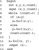
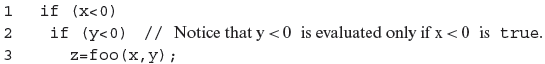
Example 7.13 To illustrate the need for decision coverage, consider P7.7. This program inputs an integer x, and if necessary, transforms it into a positive value before invoking function foo-1 to compute the output z. However, as indicated, this program has an error. Assume that as per its requirements, the program must compute z using foo-2 when x ≥ 0. Now consider the following test set Τ for this program.
T = {t1 : < x = –5 >}
It is easy to verify that when P7.7 is executed against the sole test case in T, all statements and all blocks in this program are covered. Hence Τ is adequate with respect to both the statement and the block coverage criteria. However, this execution does not force the condition inside the if to be evaluated to false thus avoiding the need to compute z using foo-2. Hence Τ does not reveal the error in this program.
Program P7.7
Suppose that we add a test case to Τ to obtain an enhanced test set T′.
T′= {t1 :< x = –5 >, t2 :< x = 3 >}
When P7.7 is executed against all tests in T′, all statements and blocks in the program are covered. In addition, the sole decision in the program is also covered because condition x < 0 evaluates to true when the program is executed against t1 and to false when executed against t2. Of course, control is diverted to the statement at line 6 without executing line 5. This causes the value of z to be computed using foo-1 and not foo-2 as required. Now, if foo-1 (3) ≠ foo-2 (3) then the program will give an incorrect output when executed against test t2.
Decision coverage aids in testing if decisions in a program are correctly formulated and located.
The above example illustrates how decision coverage might help a tester discover an incorrect condition and a missing statement by forcing the coverage of a decision. As you may have guessed, covering a decision does not necessarily imply that an error in the corresponding condition will always be revealed. As indicated in the example above, certain other program dependent conditions must also be true for the error to be revealed. We now formally define adequacy with respect to the decision coverage.
Decision coverage:
The decision coverage of Τ with respect to (P,R) is computed as |Dc|/(|De| – |Di|), where Dc is the set of decisions covered, Di the set of infeasible decisions, and De the set of decisions in the program, i. e. the decision coverage domain. Τ is considered adequate with respect to the decision coverage criterion if the decision coverage of Τ with respect to (P,R) is 1.
The coverage domain in decision coverage is the set of all possible decisions in the program under test.
The domain of decision coverage consists of all decisions in the program under test. Note that each if and each while contribute to one decision whereas a switch may contribute to more than one. For the program in Example 7.13, the decision coverage domain is De={x< 0} and hence |De | = 1.
7.2.4 Condition coverage
A decision can be composed of a simple condition such as x < 0, or of a more complex condition, such as ((x < 0 and y < 0) or (p ≥ q)). Logical operators and, or, and xor connect two or more simple conditions to form a compound condition. In addition, ¬ (pronounced as ‘not’) is a unary logical operator that negates the outcome of a condition.
Coverage of a decision does not necessarily imply the coverage of the corresponding condition. This is so when the condition is compound.
A simple condition is considered covered if it evaluates to true and false in one or more executions of the program in which it occurs. A compound condition is considered covered if each simple condition it consists of is also covered. For example, (x < 0 and y < 0) is considered covered when both x < 0 and y < 0 have evaluated to true and false during one or more executions of the program in which they occur.
Decision coverage is concerned with the coverage of decisions regardless of whether or not a decision corresponds to a simple or a compound condition. Thus in the statement
1 if (x < 0 and y < 0) 2 z = foo(x,y);
there is only one decision that leads control to line 2 if the compound condition inside the if evaluates to true. However, a compound condition might evaluate to true or false in one of several ways. For example, the condition at line 1 above evaluates to false when x ≥ 0 regardless of the value of y. Another condition such as x < 0 or y < 0 evaluates to true regardless of the value of y when x < 0. With this evaluation characteristic in view, compilers often generate code that uses short circuit evaluation of compound conditions. For example, the if statement in the above code segment might get translated into the following sequence.
In the code segment above, we see two decisions, one corresponding to each simple condition in the if statement. This leads us to the following definition of condition coverage.
Condition coverage:
The condition coverage of Τ with respect to (P,R) is computed as |Cc|/(|Ce| – |Ci|) where Cc is the set of simple conditions covered, Ci is the set of infeasible simple conditions, and Ce is the set of simple conditions in the program, i. e. the condition coverage domain. Τ is considered adequate with respect to the condition coverage criterion if the condition coverage of Τ with respect to (P,R) is 1.
The coverage domain in condition coverage is the set of all simple conditions in the program under test. Decision coverage implies condition coverage when there are no compound conditions.
Sometimes the following alternate formula is used to compute the condition coverage of a test:
where each simple condition contributes 2, 1, or 0 to Cc depending on whether it is covered, partially covered, or not covered, respectively. For example, when evaluating a test set T, if x < y evaluates to true but never to false, then it is considered partially covered and contributes a 1 to Cc.
Example 7.14 Consider the following program that inputs values of x and y and computes the output z using functions foo1 and foo2. Partial specifications for this program are given in Table 7.1. This table lists how z is computed for different combinations of x and y. A quick examination of P7.8 against Table 7.1 reveals that for x ≥ 0 and y ≥ 0 the program incorrectly computes z as foo2(x,y).
Table 7.1 Truth table for the computation of z in P7.8.
x < 0
y < 0
Output (z)
true
true
false
false
true
false
true
false
foo1(x,y)
foo2(x,y)
foo2(x,y)
foo1(x,y)
Program P7.8
1 begin
2 int x, y, z;
3 input (x, y);
4 if(x<0 and y<0)
5 z=foo1(x,y);
6 else
7 z=foo2(x,y);
8 output(z);
9 end
Consider Τ designed to test P7.8.
Τ is adequate with respect to the statement, block, and decision coverage criteria. You may verify that P7.8 behaves correctly on t1 and t2.
To compute the condition coverage of T, we note that Ce = {x < 0, y < 0}. Tests in Τ cover only the second of the two elements in Ce. As both conditions in Ce are feasible, |Ci| = 0. Plugging these values into the formula for condition coverage we obtain the condition coverage for T to be 1/(2 – 0) = 0.5.
We now add the test t3 :< x = 3, y = 4 > to T. When executed against t3, P7.8 incorrectly computes z as foo2(x,y). The output will be incorrect if foo1 (3, 4) ≠ foo2 (3 , 4). The enhanced test set is adequate with respect to the condition coverage criterion and possibly reveals an error in the program.
7.2.5 Condition/decision coverage
In the previous two sections we learned that a test set is adequate with respect to decision coverage if it exercises all outcomes of each decision in the program during testing. However, when a decision is composed of a compound condition, decision coverage does not imply that each simple condition within a compound condition has taken both values true and false.
Condition coverage ensures that each simple condition within a compound condition has assumed both values true and false. However, as illustrated in the next example, condition coverage does not require each decision to have produced both outcomes. Condition/decision coverage is also known as branch condition coverage.
Example 7.15 Consider a slightly different version of P7.8 obtained by replacing and by or in the if condition. For P7.9, we consider two test sets T1 and T2.
Program P7.9
1 begin
2 int x, y, z;
3 input (x, y);
4 if(x<0 or y<0)
5 z=foo1(x,y);
6 else
7 z=foo2(x,y);
8 output(z);
9 end
Test set T1 is adequate with respect to the decision coverage criterion because test t1 causes the if condition to be true and test t2 causes it to be false. However, T1 is not adequate with respect to the condition coverage criterion because condition y < 0 never evaluates to true. In contrast, T2 is adequate with respect to the condition coverage criterion but not with respect to the decision coverage criterion.
The condition/decision coverage based adequacy criterion is developed to overcome the limitations of using the condition and decision coverage criteria independently. A definition follows.
Condition/decision coverage:
The condition/decision coverage of Τ with respect to (P,R) is computed as (|Cc| + |Dc|)/((|Ce| – |Ci|) + (|De| – |Di|)), where Cc denotes the set of simple conditions covered, Dc the set of decisions covered, Ce and De the sets of simple conditions and decisions, respectively, and Ci and Di the sets of infeasible simple conditions and decisions, respectively. Τ is considered adequate with respect to the condition/decision coverage criterion if the condition/decision coverage of Τ with respect to (P,R) is 1.
Condition coverage does not imply decision coverage. This is true when one or more decisions in a program is made up of compound conditions.
Example 7.16 For P7.8, a simple modification of T1 from Example 7.15 gives us Τ that is adequate with respect to the condition/decision coverage criteria.
7.2.6 Multiple condition coverage
Multiple condition coverage is also known as branch condition combination coverage. To understand multiple condition coverage, consider a compound condition that contains two or more simple conditions. Using condition coverage on some compound condition C implies that each simple condition within C has been evaluated to true and false. However, it does not imply that all combinations of the values of the individual simple conditions in C have been exercised. The next example illustrates this point.
Multiple condition coverage aims at covering combinations of values of the simple conditions in a compound condition. Of course, such combinations grow exponentially with the number of simple conditions in a compound condition.
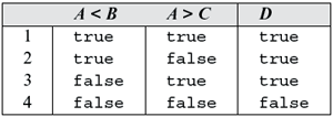
Example 7.17 Consider D = (A < B) or (A > C) composed of two simple conditions A<B and A > C. The four possible combinations of the outcomes of these two simple conditions are enumerated in Table 7.2.
Table 7.2 Combinations in D = (A < B) or (A > C).
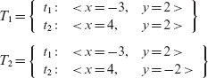
Now consider test set Τ containing two tests.
The two simple conditions in D are covered when evaluated against tests in T. However, only two combinations in Table 7.2, those at lines 1 and 4, are covered. We need two more tests to cover the remaining two combinations at lines 2 and 3 in Table 7.2. We modify Τ to T′ by adding two tests that cover all combinations of values of the simple conditions in D.
To define test adequacy with respect to the multiple condition coverage criterion, suppose that the program under test contains a total of n decisions. Assume also that each decision contains k1,k2,...,kn simple conditions. Each decision has several combinations of values of its constituent simple conditions. For example, decision i will have a total of 2ki combinations. Thus the total number of combinations to be covered is
With this background, we now define test adequacy with respect to multiple condition coverage.
Multiple condition coverage:
The multiple condition coverage of Τ with respect to (P,R) is computed as |Cc|/(|Ce| – |Ci|), where Cc denotes the set of combinations covered, Ci the set of infeasible simple combinations, and
the total number of combinations in the program. Τ is considered adequate with respect to the multiple condition coverage criterion if the multiple condition coverage of Τ with respect to (P,R) is 1.
The coverage domain for multiple condition coverage consists of all combinations of simple conditions in each compound condition in the program under test. Decisions made up of only simple conditions should also be included in this coverage domain.
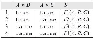
Example 7.18 It is required to write a program that inputs values of integers A, B, and C and computes an output S as specified in Table 7.3. Note from this table the use of functions f1 through f4 used to compute S for different combinations of the two conditions A < Β and A > C. P7.10 is written to meet the desired specifications. There is an obvious error in the program, computation of S for one of the four combinations, line 3 in the table, has been left out.
Table 7.3 Computing S for P7.10.
Program P7.10
1 begin
2 int A, B, C, S=0;
3 input (A, B, C);
4 if(A < B and A>C) S=f1(A, B, C);
5 if(A < B and A≤C) S=f2(A, B, C);
6 if(A ≥ B and A ≤ C) S=f4(A, B, C);
7 output(S);
8 end
Consider test set Τ developed to test P7.10; this is the same test used in Example 7.17.
P7.10 contains three decisions, six conditions, and a total of 12 combinations of simple conditions within the three decisions. Notice that because all three decisions use the same set of variables, A, B, and C, the number of distinct combinations is only four. Table 7.2 lists all four combinations.
When P7.10 is executed against tests in T, all simple conditions are covered. Also, the decisions at lines 4 and 6 are covered. However, the decision at line 5 is not covered. Thus, Τ is adequate with respect to condition coverage but not with respect to decision coverage. To improve the decision coverage of T , we obtain Τ′ by adding test t3 from Example 7.17.
T′ is adequate with respect to decision coverage. However, none of the three tests in T′ reveal the error in P7.10. Let us now evaluate whether or not T′ is adequate with respect to the multiple condition coverage criteria.
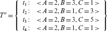
Table 7.4 lists the 12 combinations of conditions in three decisions and the corresponding coverage with respect to tests in T′. From the table we find that one combination of conditions in each of the three decisions remains uncovered. For example, at line 3 the (false, true) combination of the two conditions A < Β and A > C remains uncovered. To cover this pair we add t4 to T′ and get the following modified test set T''.
Table 7.4 Condition coverage for P7.10.
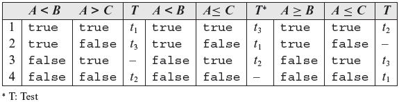
Test t4 in T'' does cover all of the uncovered combinations in Table 7.4 and hence renders T'' adequate with respect to the multiple condition criterion.
You might have guessed that our analysis in Table 7.4 is redundant. As all three decisions in P7.10 use the same set of variables, A, B, and C, we need to analyze only one decision in order to obtain a test set that is adequate with respect to the multiple condition coverage criterion.
7.2.7 Linear code sequence and jump (LCSAJ) coverage
Execution of sequential programs that contain at least one condition proceeds in pairs where the first element of the pair is a sequence of statements (a block), executed one after the other, and terminated by a jump to the next such pair (another block). The first element of this pair is a sequence of statements that follow each other textually. The last such pair contains a jump to program exit thereby terminating program execution. An execution path through a sequential program is composed of one or more of such pairs.
Test adequacy based on linear code sequence and jump aims at covering paths that might not otherwise be covered when decision, condition, or multiple condition coverage is used.
A Linear Code Sequence and Jump is a program unit comprising a textual code sequence that terminates in a jump to the beginning of another code sequence and jump. The textual code sequence may contain one or more statements. An LCSAJ is represented as a triple (X, Y, Z) where X and Y are, respectively, locations of the first and the last statement and Ζ is the location to which the statement at X jumps. The last statement in an LCSAJ is a jump and Ζ may be program exit.
When control arrives at statement X, follows through to statement Y, and then jumps to statement Z, we say that the LCSAJ (X,Y,Z) is traversed. Alternate terms for “traversed” are covered and exercised. The next three examples illustrate the derivation and traversal of LCSAJs in different program structures.
Example 7.19 Consider the following program consisting of one decision. We are not concerned with the code for function g used in this program.
Program P7.11
1 begin
2 int x, y, p;
3 input (x, y);
4 if(x<0)
5 p=g(y);
6 else
7 p=g(y*y);
8 end
Listed below are three LCSAJ’s in P7.11 . Note that each LCSAJ begins at a statement and ends in a jump to another LCSAJ. The jump at the end of an LCSAJ takes control to either another LCSAJ or to program exit.
Now consider the following test set consisting of two test cases.
When P7.11 is executed against t1, LCSAJs (1, 6, exit) are excited. When the same program is executed again test t2, the sequence of LCSAJs executed is (1, 4, 7) and (7, 8, exit). Thus, execution of P7.11 against both tests in Τ causes each of the three LCSAJs to be executed at least once.
Example 7.20 Consider the following program that contains a loop.
Program P7.12
1 begin
2 // Compute xy given non-negative integers x and y.
3 int x, y, p;
4 input (x, y);
5 p=1;
6 count=y;
7 while(count>0){
8 p=p*x;
9 count=count—1;
10 }
11 output(p);
12 end
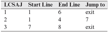
The LCSAJs in P7.12 are enumerated below. As before, each LCSAJ begins at a statement and ends in a jump to another LCSAJ.
The following test set consisting of three test cases traverses each of the five LCSAJs listed above.
Upon execution on t1, P7.12 traverses LCSAJ (1, 7, 11) followed by LCSAJ (11, 12, exit). When P7.12 is executed against t2, the LCSAJs are executed in the following sequence: (1, 10, 7) → (7, 10, 7) → (7, 7, 11)→ (11, 12, exit).
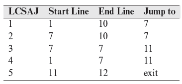
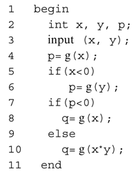
Example 7.21 Consider the following program that contains several conditions.
Program P7.13
Five LCSAJs for P7.13 follow.
The following test set consisting of two test cases traverses each of the five LCSAJs listed above.
Assuming that g(0)<0, LCSAJ 1 is traversed when P7.13 is executed against t1. In this case, the decisions at lines 5 and 7 both evaluate to true. Assuming that g(5) ≥ 0, the sequence of LCSAJs executed when P7.13 is executed against t2 is (1, 5, 7) → (7, 10, exit). Both decisions evaluate to false during this execution.
We note that the execution of P7.13 against t1 and t2 has covered both the decisions. Hence, Τ is adequate with respect to the decision coverage criterion even if test t3 were not included. However, LCSAJs 4 and 5 have not been traversed yet. Assuming that g(2)<0, the remaining two LCSAJs are traversed, LCSAJ 4 followed by LCSAJ 5, when P7.13 is executed against t3.
Example 7.21 illustrates that a test adequate with respect to decision coverage might not exercise all LCSAJs and more than one decision statement might be included in one LCSAJ, as for example is the case with LCSAJ 1. We now give a formal definition of test adequacy based on LCSAJ coverage.
The LCSAJ coverage of a test set Τ with respect to (P,R) is computed as
Τ is considered adequate with respect to the LCSAJ coverage criterion if the LCSAJ coverage of Τ with respect to (P, R) is 1.
Test adequacy based on LCSAJ’s is computed, as in other cases, as the ratio of the number of LCSAJs covered to the number of feasible LCSAJs. Note that there are multiple ways to define an LCSAJ depending on how long a sequence of code sequence and jump is one willing to consider.
7.2.8 Modified condition/decision coverage
As we learned in the previous section, multiple condition coverage requires covering all combinations of simple conditions within a compound condition. Obtaining multiple condition coverage might become expensive when there are many embedded simple conditions.
When a compound condition C contains n simple conditions, the maximum number of tests required to cover C is 2n. Table 7.5 exhibits the growth in the number of tests as n increases. The table also shows the time it will take to run all tests given that it takes 1 millisecond (ms) to set up and execute each test. It is evident from the numbers in this table that it would be impractical to obtain 100% the multiple condition coverage for complex conditions. One might ask: “Would any programmer ever devise a complex condition that contains 32 simple conditions?” Indeed, though not frequently, some avionics systems do contain such complex conditions.
The Modified condition/decision coverage is also known as MC/DC coverage. In several application domains, e.g., aerospace, tests must be demonstrated to be MC/DC adequate.
Table 7.5 Growth in the maximum number of tests required for multiple condition coverage for a condition with n simple conditions.
n |
Number of tests |
Time to execute all tests |
|---|---|---|
|
1 4 8 16 32 |
2 16 256 65536 4294967296 |
2 ms 16 ms 256 ms 65.5 seconds 49.5 days |
A weaker adequacy criterion based on the notion of modified condition decision coverage, also known as “MC/DC coverage,” allows a thorough yet practical test of all conditions and decisions. As is implied in its name, there are two parts to this criteria: the “MC” part and the “DC” part. The DC part corresponds to decision coverage discussed earlier.
The next example illustrates the meaning of the “MC” part in the MC/DC coverage criteria. Be forewarned that this example is merely illustrative of the meaning of “MC” and is not to be treated as an illustration of how one could obtain MC/DC coverage. A practical method for obtaining MC/DC coverage is given later in this section.
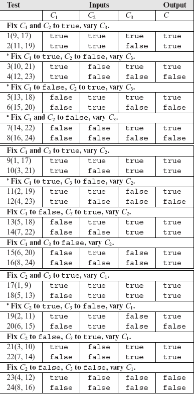
Example 7.22 To understand the “MC” portion of the MC/DC coverage, consider a compound condition C = (C1 and C2) or C3 where C1, C2, and C3 are simple conditions. To obtain MC adequacy, we must generate tests to show that each simple condition affects the outcome of C independently. To construct such tests, we fix two of the three simple conditions in C and vary the third. For example, we fix C1 and C2 and vary C3 as shown in the first eight rows of Table 7.6. There are three combinations of two simple conditions and each combination leads to eight possibilities. Thus we have a total of 24 rows in Table 7.6.
MC part of the MC/DC adequacy is demonstrated by showing that each simple condition in each decision in the program under test has an impact on the outcome of the decision. Doing so generally requires fewer tests than would be required to obtain multiple condition coverage.
Table 7.6 Test cases for C = (C1 and C2) or C3 to illustrate MC/DC coverage. Identical rows are listed in parentheses.
 *Corresponding tests affect C and may be included in the MC/DC adequate test set.
Many of these 24 rows are identical as indicated in the table. For each of the three simple conditions, we select one set of two tests that demonstrate the independent effect of that condition on C. Thus we select tests (3, 4) for C3, (11, 12) for C2, and (19, 20) for C1. These tests are shown in Table 7.7 which contains a total of only six tests. Note that we could have as well selected (5, 6) or (7, 8) for C3.
Table 7.7 MC-adequate tests for C = (C1 and C2) or C3
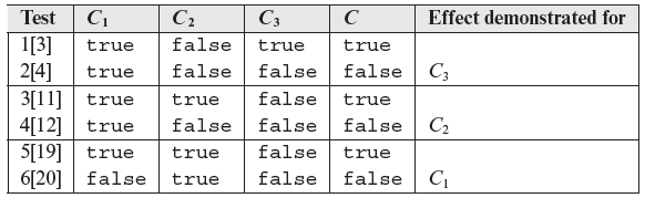
Table 7.7 also has some redundancy as tests (2, 4) and (3, 5) are identical. Compacting this table further by selecting only one amongst several identical tests, we obtain a minimal MC adequate test set for C shown in Table 7.8.
Table 7.8 Minimal MC-adequate tests for C = (C1 and C2) or C3
The key idea in Example 7.22 is that every compound condition in a program must be tested by demonstrating that each simple condition within the compound condition has an independent effect on its outcome. The example also reveals that such demonstration leads to fewer tests than required by the multiple-condition coverage criteria. For example, a total of eight tests are required to satisfy the multiple condition criteria when condition C = (C1 and C2) or C3 is tested. This is in contrast to only four tests required to satisfy the MC/DC criterion.
7.2.9 MC/DC adequate tests for compound conditions
It is easy to improve upon the brute force method of Example 7.22 for generating MC/DC adequate tests for a condition. First, we note that only two tests are required for a simple condition. For example, to cover a simple condition x < y, where x and y are integers, one needs only two tests, one that causes the condition to be true and another that causes it to be false.
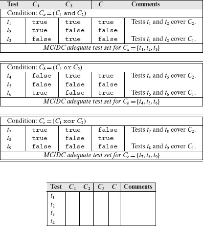
Next, determine MC/DC adequate tests for compound conditions that contain two simple conditions. Table 7.9 lists adequate tests for such compound conditions. Note that three tests are required to cover each condition using the MC/DC requirement. This number would be four if multiple condition coverage is required. It is instructive to carefully go through each of the three conditions listed in Table 7.9 and verify that indeed the tests given are independent (also try Exercise 7.14).
Fewer tests are needed constructed to satisfy the MC/DC coverage criterion than for the multiple condition coverage criterion.
Table 7.9 MC/DC adequate tests for compound conditions that contain two simple conditions.
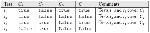
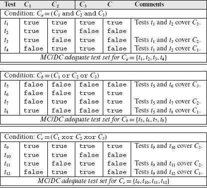
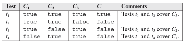
We now build Table 7.10, that is analogous to Table 7.9, for compound conditions that contain three simple conditions. Notice that only four tests are required for to cover each compound condition listed in Table 7.10. One can generate the entries in Table 7.10 from Table 7.9 by using the following procedure which works for a compound condition C that is a conjunct of three simple conditions, i.e. C = (C1 and C2 and C3).
There is a simple procedure for finding combinations of truth values of simple conditions that satisfy MC/DC criteria. Of course, actual tests need to be derived from these truth values.
Table 7.10 MC/DC adequate tests for compound conditions that contain three simple conditions.
- Create a table with four columns and four rows. Label the columns as Test, C1, C2, C3, and C, from left to right. The column labeled Test contains rows labeled by test case numbers t1 through t4. The remaining entries are empty. The last column labeled Comments is optional.
- Copy all entries in columns C1, C2, and C from Table 7.9 into columns C2, C3, and C of the empty table.
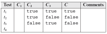
- Fill the first three rows in the column marked C1 with true and the last row with false.
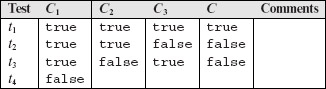
- Fill entries in the last row under columns labeled C2, C3, and C with true, true, and false, respectively.
- We now have a table containing MC/DC adequate tests for C = (C1 and C2 and C3) derived from tests for C= (C1 and C2).
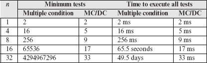
The procedure illustrated above can be extended to derive tests for any compound condition using tests for a simpler compound condition (see Exercises 7.15 and 7.16). The important point to note here is that for any compound condition, the size of an MC/DC adequate test set grows linearly in the number of simple conditions. Table 7.5 is reproduced below with columns added to compare the minimum number of tests required, and the time to execute them, for multiple condition and MC/DC coverage criteria.
7.2.10 Definition of MC/DC coverage
We now provide a more complete definition of the MC/DC coverage. A test set Τ for program P written to meet requirements R is considered adequate with respect to the MC/DC coverage criterion if upon the execution of P on each test in T, the following requirements are met.
An MC/DC adequate test set covers all decisions, all simple conditions, and has demonstrated the effect of each simple condition on the outcome of the decision in which the simple condition is embedded.
- Each block in P has been covered.
- Each simple condition in P has taken both true and false values.
- Each decision in P has taken all possible outcomes.
- Each simple condition within a compound condition C in P has been shown to independently effect the outcome of C. This is the MC part of the coverage we discussed in detail earlier in this section.
The first three requirements above correspond to block, condition, and decision coverage, respectively, and have been discussed in earlier sections. The fourth requirement corresponds to “MC” coverage discussed earlier in this section. Thus the MC/DC coverage criterion is a mix of four coverage criteria based on the flow of control. With regard to the second requirement, it is to be noted that conditions that are not part of a decision, such as the one in the following statement
A = (p <q) or (x >y)
are also included in the set of conditions to be covered. With regard to the fourth requirement, a condition such as (A and B) or (C and A) poses a problem. It is not possible to keep the first occurrence of A fixed while varying the value of its second occurrence. Here the first occurrence of A is said to be coupled to its second occurrence. In such cases, an adequate test set need only demonstrate the independent effect of any one occurrence of the coupled condition.
Table 7.11 MC/DC adequacy and the growth in the least number of tests required for a condition with n simple conditions.
There are multiple ways of quantitatively measuring MC/DC adequacy. One way is to treat separately each of the individual requirements in the MC/DC criterion. The other way is to create a single metric.
A numerical value can also be associated with a test to determine the extent of its adequacy with respect to the MC/DC criterion. One way to do so is to treat separately each of the four requirements listed above for MC/DC adequacy. Thus, four distinct coverage values can be associated with T, namely, block coverage, condition coverage, decision coverage, and MC coverage. The first three of these four have already been defined earlier. A definition of MC coverage follows.
Let C1, C2, … , CN be the conditions in P; each condition could be simple or compound and may or may not appear within the context of a decision. Let ni denote the number of simple conditions in Ci, ei the number of simple conditions shown to have independent affect on the outcome of Ci, and fi the number of infeasible simple conditions in Ci. Note that a simple condition within a compound condition C is considered infeasible if it is impossible to show its independent affect on C while holding constant the remaining simple conditions in C. The MC coverage of Τ for program P subject to requirements R, denoted by MCc, is computed as follows.
Thus, test set Τ is considered adequate with respect to the MC coverage if MCcof T is 1. Having now defined all components of the MC/DC coverage, we are ready for a complete definition of the adequacy criterion based on this coverage.
Modified condition/decision coverage:
A test Τ to test program P subject to requirements R is considered adequate with respect to the MC/DC coverage criterion if Τ is adequate with respect to block, decision, condition, and MC coverage.
The next example illustrates the process of generating MC/DC adequate tests for a program that contains three decisions, one composed of a simple condition and the remaining two composed of compound conditions.
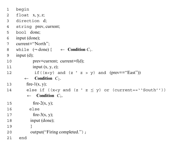
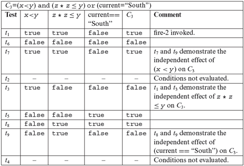
Example 7.23 P7.14 is written to meet the following requirements.
R1: Given coordinate positions x, y, and z, and a direction value d, the program must invoke one of the three functions fire-1, fire-2, and fire-3 as per conditions below.
R1.1: Invoke fire-1 when (x<y) and (z * z > y) and (prev=“East”), where prev and current denote, respectively, the previous and current values of d.
R1.2: Invoke fire-2 when (x<y) and (z * z ≤ y) or (current=“South”).
R1.3: Invoke fire-3 when none of the two conditions above is true.
R2: The invocation described above must continue until an input Boolean variable becomes true.
Program P7.14
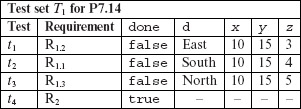
First we generate tests to meet the given requirements. Three tests derived to test R1.1, R1.2, and R1.3 follow; note that these tests are to be executed in the sequence listed.
Assuming that P7.14 has been executed against the tests given above, let us analyze which decisions have been covered and which ones have not been covered. To make this task easy, the values of all simple and compound conditions are listed below for each test case.
Test |
C1 |
Comment |
|---|---|---|
|
t1 |
true |
C2=false, C3=true, hence fire-2 invoked. |
|
t2 |
true |
C2=true, hence fire-1 invoked. |
|
t3 |
true |
Both C2 and C3 are false, hence fire-3 invoked. |
|
t4 |
false |
This terminates the loop. The decision at line 8 is covered. |
First, it is easy to verify that all statements in P7.14 are covered by test set T1. This also implies that all blocks in this program are covered. Next, a quick examination of the tables above reveals that the three decisions at lines 8,12, and 14 are also covered as both outcomes of each decision have been taken. Condition C1 is covered by tests t1 and t4 and also by tests t2 and t4, and by t3 and t4. However, compound condition C2 is not covered because x < y is not covered. Also, C3 is not covered because (x<y) is not covered. This analysis leads to the conclusion that T1 is adequate with respect to the statement, block, and decision coverage criteria but not with respect to the condition coverage criteria.
Next we modify T1 to make it adequate with respect to the condition coverage criteria. Recall that C2 is not covered because x<y is not covered.
To cover x<y we generate a new test t5 and add it to T1 to obtain T2 given below. The value of x being greater than that of y which makes x<y false. Also, we looked ahead and set d to “South” to make sure that (current == “South”) in C3 evaluates to true. Note the placement of t5 with respect to t4 to ensure that the program under test is executed against t5 before it is executed against t4 or else the program will terminate without covering x<y.
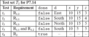
The evaluations of C2 and C3 are reproduced below with a row added for the new test t5. Note that test T2, obtained by enhancing T1, is adequate with respect to the condition coverage criterion. Obviously, it is not adequate with respect to the multiple condition coverage criteria. Such adequacy will imply a minimum of eight tests and the development of these is left to Exercise 7.21.
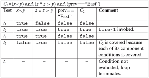
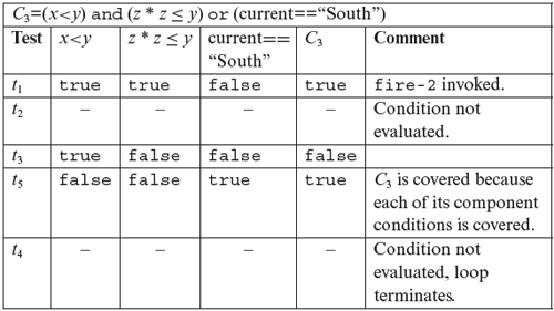
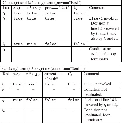
Next, we check if T2 is adequate with respect to the MC/DC criterion. From the table given above for C2, we note that conditions (x<y) and (z*z>y) are kept constant in t2 and t3, while (prev==“East”) is varied. These two tests demonstrate the independent effect of (prev==“East”) on C2. However, the independent effect of the remaining two conditions is not demonstrated by T2. In the case of C3, we note that in tests t1 and t3, conditions (x<y) and (current==“South”) are held constant while (z* z≤y) is varied. These two tests demonstrate the independent effect of (z* z≤y) on C3. Tests t1 and t3 demonstrate the independent effect of (z* z≤y) on C3. However, the independent effect of (current==“South”) on C3 is not demonstrated by T2. This analysis reveals that we need to add at least two tests to T2 to obtain MC/DC coverage.
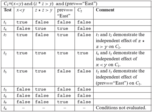
To obtain MC/DC coverage for C2, consider (x<y). We need two tests that fix the remaining two conditions, vary (x<y), and cause C2 to be evaluated to true and false. We reuse t2 as one of these two tests. The new test must hold (z* z>y) and (prev==“East”) to true and make (x<y) evaluate to false. One such test is t6, to be executed right after t1 but before t2. Execution of the program against t6 causes (x<y) to evaluate to false and C2 also to false. t6 and t2 together demonstrate the independent effect of (x<y) on C2. Using similar arguments, we add test t7 to show the independent effect of (z* z>y) on C2. Adding t6 and t7 to T2 gives us an enhanced test set T3.
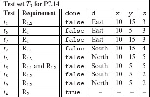
Upon evaluating C3 against the newly added tests, we observe that the independent effects of (x<y) and (z* z ≤ y) have been demonstrated. We add t8and t9 to show the independent effect of (current==“South”) on C3. The complete test set, T3 listed above, is MC/DC adequate for P7.14. Once again, note the importance of test sequencing. t1 and t7 contain identical values of input variables but lead to different effects in the program due to their position in the sequence in which tests are executed. Also note that test t2 is of no use for covering any portion of C3 because C3 is not evaluated when the program is executed against this test.
7.2.11 Minimal MC/DC tests
In Example 7.23, we did not make any effort to obtain the smallest test set adequate with respect to the MC/DC coverage. However, while generating tests for large programs involving several compound conditions, one might like to generate the smallest number of MC/DC adequate tests. This is because execution against each test case might take a significant chunk of test time, e.g. 24 hours! Such execution times might be considered exorbitant in several development environments. In situations like this, one might consider using one of several techniques for the minimization of test sets. Such techniques are discussed in Chapter 9.
MC/DC tests generated using techniques described earlier might not be minimal. Thus, it may be possible to discard some of these tests without affecting the test adequacy. Such reduction can be achieved using techniques discussed elsewhere in this book.
7.2.12 Error detection and MC/DC adequacy
In Example 7.14, we saw how obtaining condition coverage led to a test case that revealed a missing condition error. Let us now dwell on what types of errors might one find while enhancing tests using the MC/DC criterion. In this discussion we assume that the test being enhanced is adequate with respect to condition coverage but not with respect to MC/DC coverage, and has not revealed an error. Consider the following three error types in a compound condition; errors in simple conditions have been discussed in Section 7.2.3.
Missing condition: One or more simple conditions is missing from a compound condition. For example, the correct condition should be (x<y and done) but the condition coded is (done).
Incorrect Boolean operator: One or more Boolean operators is incorrect. For example, the correct condition is (x<y and done) which has been coded as (x<y or done).
Mixed type: One or more simple conditions is missing and one or more Boolean operators is incorrect. For example, the correct condition should be (x<y and z * x>y and d=“South”) has been coded as (x<y or z * x≥y).
Note that we are considering errors in code. We assume that we are given a test set Τ for program P subject to requirements R. Τ is adequate with respect to the condition coverage criterion. The test team has decided to enhance Τ to make it adequate with respect to the MC/DC coverage criterion. Obviously the enhancement process will lead to the addition of zero or more tests to T; no tests will be added if Τ is already MC/DC adequate.
We also assume that P contains a missing condition error or an incorrect Boolean operator error. The question we ask is: “Will the enhanced Τ detect the error?” In the three examples that follow, we do not consider the entire program, instead, we focus only on the erroneous condition (see Exercise 7.25).
Example 7.24 Suppose that condition C = C1 and C2 and C3 has been coded in a program as C′= C1 and C3. The first two tests below form a test set adequate with respect to condition coverage for C′. The remaining two tests, when combined with the first two, constitute an MC/DC adequate test for C′. Note that the adequate test set is developed for the condition as coded in the program, and not the correct condition.
There is no guarantee that an MC/DC adequate test set will be able to detect a missing-condition error.
The first two tests do not reveal the error as both C and C′ evaluate to the same value for each test. The next two tests, added to obtain MC/DC coverage, also do not detect the error. Thus, in this example, an MC/DC adequate test is unable to detect a missing-condition error.
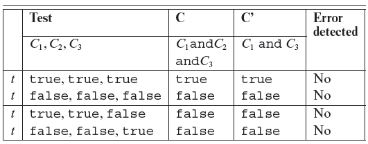
It should be noted in the above example that the first two tests are not adequate with respect to the condition coverage criterion if short-circuit evaluation is used for compound conditions. Of course, this observation does not change the conclusion we arrived at. This conclusion can be generalized for a conjunction of n simple conditions (see Exercise 7.24).
Test adequacy is affected by short-circuit evaluation of conditions. For example, a test set might be adequate with respect to the condition coverage criterion in the absence of short-circuit evaluation but not otherwise.
Example 7.25 Suppose that condition C = C1 and C2 and C3 has been coded as C′ = (C1 or C2) and C3. Six tests that form an MC/DC adequate set are in the following table. Indeed, this set does reveal the error as t7.12 and t7.12 cause C and C′ to evaluate differently. However, the first two tests do not reveal the error. Once again, we note that the first two tests below are not adequate with respect to the condition coverage criterion if short-circuit evaluation is used for compound conditions.
Example 7.26 Suppose that condition C = C1 or C2 or C3 has been coded as C = C1 and C3. Four MC/DC adequate tests are given below. All but t7.12 reveal the error.
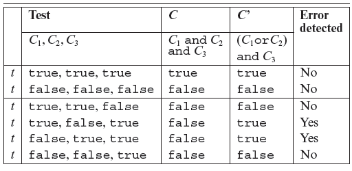
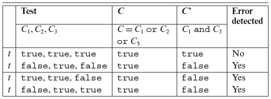
Not surprisingly, examples given above show that satisfying the MC/DC adequacy criteria does not necessarily imply that errors made while coding conditions will be revealed. However, the examples do favor MC/DC over condition coverage. The first two tests in each of the three examples above are also adequate with respect to decision coverage. Hence these examples also show that an MC/DC adequate test will likely reveal more errors than a decision or condition-coverage adequate test. Note the emphasis on the word “likely.” MC/DC adequacy does not guarantee the detection of errors in an incorrectly coded condition.
It can be shown that MC/DC adequate tests have superior error detection ability than those adequate only with respect to the condition coverage criterion.
7.2.13 Short-circuit evaluation and infeasibility
Short-circuit evaluation refers to the method of partially evaluating a compound condition whenever it is sufficient to do so. It is also known as lazy evaluation. C requires short-circuit evaluation and Java allows both.
For example, consider the following decision comprising a conjunction of conditions: (C1 and C2).
Short-circuit evaluation of predicates might lead to infeasible elements in a coverage domain.
The outcome of the above condition does not depend on C2 when C1 is false. When using short-circuit evaluation, condition C2 is not evaluated if C1 evaluates to false. Thus the combination C1 = false and C2 = true, or the combination C1 = false and C2 = false, may be infeasible if the programming language allows, or requires as in C, short-circuit evaluation.
Dependence of one decision on another might also lead to an infeasible combination. Consider, for example, the following sequence of statements.
Dependence of a decision on other might lead to infeasible elements in a coverage domain.
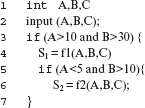
Clearly, the decision on line 5 is infeasible because the value of A cannot simultaneously be more than 10 and less than 5. However, suppose that line 3 is replaced by the following statement that has a side effect due to a call to the function foo().
3 if (A >10 and foo ()) {
Given that the execution of foo() may lead to a modification of A, the condition on line 5 is feasible.
Note that feasibility is different from reachability. A decision might be reachable but not feasible, and vice versa. In the sequence above, both the decisions are reachable but the second decision is not feasible. Consider the following sequence.
A decision might be feasible but not reachable. Alternately a decision might be infeasible though reachable. Other combinations of reachability and feasibility can also be considered.
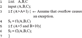
In this case, the second decision is not reachable due to an error at line 3. It may, however, be feasible.
7.2.14 Basis path coverage
Recall that a basis set is a collection of linearly independent basis paths. The construction of basis paths is introduced in Chapter 4. Basis path coverage is simply the ratio of the number of basis paths tested to the number of feasible basis paths.
Covering all basis paths implies the coverage of all feasible decisions and hence all statements. In the presence of loops, the number of paths in a program might be simply too large to obtain a complete path coverage. Basis paths offer a practical means to select a subset of all paths to cover (se Exercise 7.29).
7.2.15 Tracing test cases to requirements
When enhancing a test set to satisfy a given coverage criterion, it is desirable to ask the following question: What portions of the requirements are tested when the program under test is executed against the newly added test case? The task of relating the new test case to the requirements is known as test trace-back.
It is important that a new test case designed to cover a portion of the code be traced back to the corresponding requirements. Doing so will obviously reveal what requirement is tested by a given test case and should be the expected output.
Trace-back has at least the following advantages. One, it assists us in determining whether or not the new test case is redundant. Second, it has the likelihood of revealing errors and ambiguities in the requirements. Third, it assists with the process of documenting tests against requirements. Such documentation is useful when requirements are modified. Modification of one or more requirements can simultaneously lead to a modification of the associated test cases thereby avoiding the need to do a detailed analysis of the modified requirements.
The next example illustrates how to associate a test, generated to satisfy a coverage criterion, to the requirements. The example also illustrates how a test generated to satisfy a coverage criterion might reveal an error in the requirements or in the program.
Example 7.27 The original test set T1 in Example 7.23 contains only four tests, t1, t2, t3, and t4. T2 is obtained by enhancing T1 through the addition of t5. We ask, “Which requirement does t5 correspond to?” Recall that we added t5 to cover the simple condition x < y in C2 and C3. Going back to the requirements for P7.14, we can associate t5 with R1.1 and R1.2.
One might argue that there is nothing explicit in the requirements for P7.14 that suggest a need for t5. If one were to assume that the given requirements are correct, then indeed this argument is valid and there is no need for t5. However, in most software development projects, requirements are often incorrect, incomplete, and ambiguous. It is therefore desirable to extract as much information from the requirements as one possibly can, to generate new tests. Let us re examine R1.2 in Example 7.23 reproduced below for convenience.
R1.2: Invoke fire-2 when (x< y) and (z * z ≤ y) or (current=“South”).
Note that R1.2 is not explicit about what action to take when (current=“South”) is false. Of course, as stated, the requirement does imply that fire-2 is not to be invoked when (current=“South”) is false. Shall we go with this implication and not generate t5? Or, shall we assume that R1.2 is ambiguous and hence we do need a test case to test explicitly that indeed the program functions correctly when (current=“South”) is false? It is often safer to make the latter assumption. Of course, selecting the former assumption is less expensive in terms of the number of tests, the time to execute all tests, and the effort required to generate, analyze, and maintain the additional tests.
Moving further, one might ask, “What error in the program might be revealed by t5 that will not be revealed by executing the program against all tests in T1?” To answer this question, suppose that line 14 in P7.14 was incorrectly coded as given below while all other statements were coded as shown.
14 else if (x < y and (z * z ≤ y)
Clearly, now P7.14 is incorrect because the invocation of fire-2 is independent of (current=“South”). Execution of the incorrect program against tests in T1 will not reveal the error because all tests lead to correct response independent of how (current=“South”) evaluates. However, execution of the incorrect P7.14 against t5 causes the program to invoke fire-3 instead of invoking fire-2, and hence the error is revealed. This line of argument stresses the need for t5 generated to explicitly test (current=“South”).
An adamant tester might continue with the argument that t5 was generated to satisfy the condition coverage criterion and was not based upon the requirements; it was through an examination of the code. If the code for P7.14 was incorrect due to the incorrect coding of C3, then this test might not be generated. To counter this argument, suppose that R1.2 as stated earlier is incorrect; its correct version is
R1.2: Invoke fire-2 when (x< y) and (z * z≤ y).
Notice that now the program is correct but the requirements are not. In this case, for all tests in T1, P7.14 produces the correct response and hence the error in requirements is not revealed. However, as mentioned in Example 7.23, t5 is generated with the intention of covering both x < y and (current==“South”). When program P7.14 is executed against t5 it invokes fire-3 but the requirements imply the invocation of fire-2. This mismatch in the program response and the requirements will likely lead to an analysis of the test results and discovery of the error in the requirements.
The above discussion justifies the association of tests t5, t6, t7, t8, and t9 to requirement R1. It also stresses the need for the trace-back of all tests to requirements.
7.3 Concepts From Data Flow
So far we have considered flow of control as the basis for deriving test adequacy criteria. We examined various program constructs that establish flow of control and that are susceptible to mistakes by programmers. Ensuring that all such constructs have been tested thoroughly is a major objective of test adequacy based on flow of control. However, testing all conditions and blocks of statements is often inadequate as the test does not reveal all errors.
Control flow based adequacy criteria focus on selecting coverage domains based on the flow of control in a program. Data flow based coverage criteria focus on the flow of data for selecting coverage domains. While both strategies for determining test adequacy aid in the selection of a subset of all program paths to be tested, adequacy criteria based on data flows are generally more powerful than those based on control flows.
Another kind of adequacy criteria are based on the flow of data through the program. Such criteria focus on definitions of data and their subsequent use and are useful in improving the tests adequate with respect to criteria based on the flow of control. The next example exposes an essential idea underlying data flow based adequacy assessment.
Example 7.28 The following program inputs integers x and y, and outputs z. The program contains two simple conditions. As shown, there is an error in this program at line 8. An MC/DC adequate test follows the program.
Program P7.15
The two test cases above cover both conditions in P7.15. Note that the program initializes z on line 4 and then adjusts its value in subsequent statements depending on the values of x and y. Test t1 follows a path that traverses updates of z on line 7 followed by another on line 10. Test t2 follows a different path that traverses updates of z on line 6 followed by another update on line 9. These two tests cause the value of z, set at at line 4, to be used at lines 6 and 7 in the expression on the corresponding right hand sides.
Just as z is defined at line 4, it is also defined subsequently at lines 6, 7, 9, and 10. However, the two MC/DC adequate tests do not force the definition of z at line 6 to be used at line 9. A divide-by-zero exception would occur if the value of z were allowed to flow from line 6 to line 9. Though this exception is not caused by the value of z, forcing this path causes the program to fail.
An MC/DC adequate test set might not cover all feasible data flows in a program. Thus, any errors due to incorrect data flows might miss detection by a test that is MC/DC adequate but not adequate with respect to a data flow based adequacy criterion.
An MC/DC adequate test does not force the execution of this path and hence the error is not revealed. However, the error in this program would be revealed if the test is required to ensure that each feasible definition and use pair for z is executed. One such test follows.
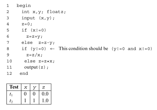
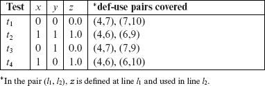
It is easy to see that an LCSAJ adequate test set would have also revealed the error in P7.15, though an MC/DC adequate test might not. In the remainder of this section, we will offer examples where an LCSJ adequate test will also not guarantee that an error is revealed but a dervied test set based on data flow will.
7.3.1 Definitions and uses
A program written in a procedural language, such as C and Java, contains variables. Variables are defined by assigning values to them and are used in expressions. An assignment statement such as
x = y+ z;
defines the variable x. This statement also makes use of variables y and z. The following assignment statement
x = x + y;
defines x as well as uses it in the right hand side expression. Declarations are assumed to be definitions of variables. For example, the declaration
int x, y, A[10];
defines three variables x, y, A[10]. An input function, such as a scanf in C, also serves to define one or more variables. For example, the statement
scanf (“%d%d”, &x, &y);
defines variables xand y. Similarly, the C statement
printf (“Output: %d n”, x + y);
uses, or refers to, variables xand y. A parameter x, passed as call-by-value to a function, is considered as a use of, or a reference to, x. A parameter x passed as call-by-reference serves as a definition and use of x. Consider the following sequence of statements that use pointers.
A variable is considered defined when the result of a computation is assigned to it. In OO languages, a name is also considered defined when an object is assigned to it. For example, using the “new” command in Java a new object can be created and assigned to a name. At this point in the code the name is considered defined.
z =&x;
y =z+1;
*z =25;
y =*z+1;
The first of the above statements defines a pointer variable z, the second defines y and uses z, the third defines x through the pointer variable z, and the last defines y and uses x accessed through the pointer variable z. Arrays are also tricky. Consider the following declaration and two statements in C:
A variable could be defined through the use of statements such as assignment state, an input statement, via parameter transfer. A variable is considered to be used when it appears in the right hand side of an assignment, or in a condition or in an output statement.
int A[10];
A[i]=x+y;
The first statement defines variable A. The second statement defines A and uses i, x, and y. One might also consider the second statement as defining only A[i] and not the entire array A. The choice of whether to consider the entire array A as defined or the specific element depends upon how stringent is the requirement for coverage analysis (see Exercise 7.28).
7.3.2 C-use and p-use
Uses of a variable that occur within an expression as part of an assignment statement, in an output statement, as a parameter within a function call, and in subscript expressions are classified as c-use, where the “c” in c-use stands for computational. There are five c-uses of x in the following statements.
A use of a variable is considered to be c-use (or computational use) when it appears inside a computation such as in an arithmetic expression. When the use appears in a condition the use is considered a p-use (or predicate use).
z = x + 1;
A[x–1]=B[2];
foo(x*x);
output(x);
An occurrence of a variable in an expression used as a condition in a branch statement, such as an if and a while, is considered a p-use. The “p” in p-use stands for predicate. There are two p-uses of z in the statements below.
if(z>0){output (x)};
while(z>x){…};
It might be confusing to classify some uses. For example, in the statement:
if(A[x+1] >0){output (x)};
the use of A is clearly a p-use. However, is the use of x within the subscript expression also a p-use? Or, is it a c-use? The source of confusion is the position of x within the if statement. x is used in an expression that computes the index value for A; it does not directly occur inside the if condition such as in if (x>0){…}. Hence, one can argue both ways: this occurrence of x is a c-use because it does not affect the condition directly, or that this occurrence of x is a p-use because it occurs in the context of a decision.
7.3.3 Global and local definitions and uses
A variable might be defined in a block, used, and redefined within the same block. Consider a block containing three statements:
p =y+z;
x =p+1;
p =z* z;
This block defines p, uses it, and redefines it. The first definition of p is local. This definition is killed, or masked, by the second definition within the same block and hence its value does not survive beyond this block. The second definition of p is a global definition as its value survives the block within which it is defined and is available for use in a subsequently executed block. Similarly, the first use of p is a local use of a definition of p that precedes it within the same block.
When a variable is defined multiple times inside a basic block, only the effect of the last definition "flows out" of the defining block. This last definition is also known as global while the ones prior to it are considered local.
The c-uses of variables y and z are global uses because the definitions of the corresponding variables do not appear in the same block preceding their use. Note that the definition of x is also global. In the remainder of this chapter, we will be concerned only with the global definitions and uses. Local definitions and uses are of no use in defining test adequacy based on data flows.
The terms “global” and “local” are used here in the context of a basic block within a program. This is in contrast to the traditional uses of these terms where a global-variable is one declared outside, and a local variable within a function or a module.
7.3.4 Data flow graph
A data flow graph of a program, also known as def-use graph, captures the flow of definitions across basic blocks in a program. It is similar to a control flow graph of a program in that the nodes, edges, and all paths through the control flow graph are preserved in the data flow graph.
A data flow graph of a program captures the data flows, i.e. the relationships between all the definitions and uses in a program. The graph can be derived from the control flow graph of a program.
A data flow graph of a program can be derived from its control flow graph. To understand how, let G = (Ν, E) be the control flow graph of program P, where Ν is the set of nodes and Ε the set of edges in the graph. Recall that each node in the control flow graph corresponds to a distinct basic block in P. We denote these blocks by b1, b2, . . . ,bk, assuming that P contains k > 0 basic blocks.
Let defi denote the set of variables defined in block i. A variable declaration, an assignment statement, an input statement, a call-by-reference parameter are program constructs that define variables. Let c-usei denote the set of variables that have a c-use in block i, and p-usei the set of variables that occur as a p-use in block i. The definition of variable x at node i is denoted by di(x). Similarly, the use of variable x at node i is denoted by ui(x). Recalling that we consider only the global definitions and uses, consider the following basic block b that contains two assignments and a function call.
p=y+z;
foo(p+q, number); // Parameters passed by value.
A[i]=x+1;
if(x>y){…};
For this basic block, we obtain defb = {p,A}, c-useb = {y, z, p, q, x, number, i}, and p-useb = {x, y}. We follow the procedure below to construct a data flow graph given program P and its control flow graph.
|
Step 1 |
Construct defi, c-usei, and p-usei for each basic block i in P. |
|
Step 2 |
Associate each node i in Ν with defi, c-usei, and p-usei. |
|
Step 3 |
For each node i that has a non-empty p-use set and ends in condition C, associate edges (i, j) and (i, k) with C and !C, respectively, given that edge (i, j) is taken when the condition is true and (i, k) taken when the condition is false. |
The next example applies the procedure given above to construct a data flow graph in Figure 7.4.
Example 7.29 First we compute the definitions and uses for each block in Figure 7.4 and associate them with the corresponding nodes and edges of the control flow graph. The def and use sets for the five blocks in this program are given below. Note that the infeasible block 4 does not affect the computation of these sets.
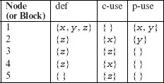
The def-set of a block is the set of all variables defined in that block. The c-use and the p-use sets of a block include, respectively, all the c- and p-uses in that block.
Using the def and use sets derived above, and the flow graph in Figure 7.4, we draw the data flow graph of P7.4 in Figure 7.6. Comparing the data flow graph with the control flow graph in Figure 7.4, we note that nodes are represented as circles with block numbers on the inside, each node is labeled with the corresponding def and use sets, and each edge is labeled with a condition. We have omitted the p-use set when it is empty, such as for nodes 3, 4, and 5. p-uses are often associated with edges in a data flow graph.
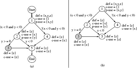
Figure 7.6 Data flow graph of 7.8 (a) start and Exit nodes shown explicitly. No def and use sets are associated with these nodes, (b) Nodes 1 and 5 serve as start and end nodes, respectively. Node 3 is shaded to emphasize that it is unreachable.
As shown in Figure 7.6 we associate p-uses with nodes that end in a condition, such as in an if or a while statement. Each variable in this p-use set also occurs along the two edges out of its corresponding node. Thus variables x and y belong to the p-use set for node 1 and also appear in the conditions attached to the outgoing edges of node 1.
As shown in Figure 7.6(b), the Start node may be omitted from the data flow graph if there is exactly one program block with no edge entering.
Similarly, the End node may be omitted in Figure 7.6 and use nodes 1 and 5 as the start and end nodes, respectively.
7.3.5 Def-clear paths
A data flow graph can have many paths. One class of paths of particular interest is known as the def-clear path. Suppose that variable x is defined at node i and there is a use of x at node j. Consider path p = (i,n1,n2, … ,nk, j), k≥0, that starts at node i, ends at node j, and nodes i and j do not occur along the subpath n1, n2, . . . , nk. p is a def-clear path for variable x defined at node i and used at node j if xis not defined along the subpath n1, n2, . . . ,nk. In this case, we also say that the definition of xat node i, i.e. di(x), is live at node j.
A def-clear path from a definition of a variable, say x, to its use is a path along which x is not redefined.
Of course, multiple definitions of a variable could be live at a specific point in the program. However, each of these definitions will flow to this point along a different path. Hence, at most one definition of a variable can be live when control arrives at a specific point in the program where that variable is used.
Note that several definitions of variable x may be live at some node j where x is used, but along different paths. Also, at most one definition could be live when control does arrive at node j where xis used.
Example 7.30 Consider the data flow graph for Program P7.16 shown in Figure 7.7. Path p = (1, 2, 5, 6) is def-clear with respect to d1(x) and u6(x). Thus d1(x) is live at node 6. Path p is not def-clear with respect to d1(z) and u6(z) due to the existence of d5(z). Also, path p is def-clear with respect to d1(count) and u6(count).
Figure 7.7 Data flow graph of Program P7.16.
Path q = (6, 2, 5, 6) is def-clear with respect to d6(count) and d6(count) (see Exercise 7.32). Variables y and z are used at node 4. It is easy to verify that definitions d1(y), d6(y), d1(z), d5(z) are live at node 4.
Program P7.16
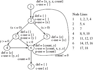
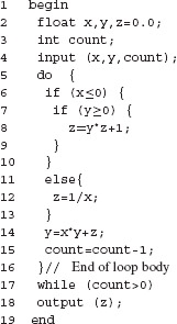
The definition of a variable at some point 11 in a program and its use at some point 12 in the same program constitute a def-sue pair. Note that 11 and 12 could be the same statements in a program.
7.3.6 Def-use pairs
We saw earlier that a def-use pair captures a specific definition and its use for a variable. For example, in P7.4, the definition of x at line 4 and itsuse at line 9 together constitute a def-use pair. The data flow graph of a program contains all def-use pairs for that program.
We are interested in two types of def-use pairs: those that correspond to a definition and its c-use, and those that correspond to a definition and its p-use. Such def-use pairs are captured in sets named dcu and dpu.
A def-use pair is placed in the dcu set if the use in the pair is a c-use, else it is placed in set dpu. Set dcu consists of all locations in a program where a specific definition of a variable has a c-use. For each definition of a variable, set dpu contains edges (k, 1) such that there is a path from where the variable is defined to location 1; location k is where the p-use occurs.
There is one dcu and one dpu set for each variable definition. For di(x), dcu(di(x)) is the set of all nodes j such that there exists uj(x) and there is a def-clear path with respect to x from node i to node j. dcu(x, i) is an alternate notation for dcu(di(x)).
When uk(x) occurs in a predicate, dpu(di(x)) is the set of edges (k, l) such that there is a def-clear path with respect to x from node i to node l. Note that the number of elements in a dpu set will be a multiple of two. dpu(x, i) is an alternate notation for dpu(di(x)).
Example 7.31 We compute the dcu and dpu sets for the data flow graph in Figure 7.7. To begin, let us compute dcu(x, 1) which corresponds to the set of all c-uses associated with the definition of x at node 1. We note that there is a c-use of x at node 5 and a def-clear path (1, 2, 5) from node 1 to node 5. Hence node 5 is included in dcu(x, 1). Similarly, node 6 is also included in this set. Thus we get dcu(x, 1)={5, 6}.
Next, determine dpu(x, 1). There is a p-use of x at node 2 with outgoing edges (2, 3) and (2, 5). The existence of def-clear paths from node 1 to each of these two edges is easily seen in the figure. There is no other p-use of x and hence we get dpu(x, 1)={(2, 3), (2, 5)}. The remaining dcu and dpu sets are given below.
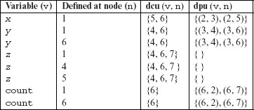
7.3.7 Def-use chains
A def-use pair consists of a definition of a variable in some block and its use in another block in the program. The notion of def-use pair can be extended to a sequence of alternating definitions and uses of variables. Such an alternating sequence is known as a def-use chain, or a k-dr interaction. The nodes along this alternating sequence are distinct. The k in k-dr interaction denotes the length of the chain and is measured in the number of nodes along the chain which is one more than the number of def-use pairs along the chain. The letters d and r refer to, respectively, definition and reference. Recall that we use the terms “reference” and “uses” synonymously.
A def-use chain a an alternating sequence of def-use pairs for a specific variable. Another name for a def-use chain is a k-dr interaction, k being the length of the chain.
Example 7.32 In Program P7.16, we note the existence of d1(z) and u4(z). Thus the def-use interaction for variable z at nodes 1 and 4 constitutes a k-dr chain for k = 2. This chain is denoted by the pair (1, 4).
A longer chain (1, 4, 6) is obtained by appending d4(z) and u6(z) to (1, 4). Note that there is no chain for k > 3 that corresponds to alternating def-uses for z. Thus, for example, path (1, 4, 4, 6) for k = 4 corresponding to the def-use sequence (d1(z), u4(z), d4(z), u6(z)) is not a valid k-dr chain due to the repetition of node 4.
The chains in the above example correspond to the definition and use of the same variable z. k-dr chains could also be constructed from alternating definitions and uses of variables not necessarily distinct. In general, a k-dr chain for variables x1, x2, … ,xk−1 is a path (n1, n2, ... ,nk) such that there exist dni(Xi) and uni+1(xi) for 1 ≤ i < k, and there is a definite clear path from ni to ni+1. This definition of a k-dr chain implies that variable xi+1 is defined in the same node as variable xi. A chain may also include the use of a variable in a predicate.
Example 7.33 Once again, let us refer to Program P7.16 and consider variables yand z. The triple (5, 6, 4) is a k-dr chain of length 3. It corresponds to the alternating sequence (d5(z), u6(z), d6(y), u4(y)). Another chain (1, 4, 6) corresponds to the alternating sequence (d1(y), u4(y), d4(z), u6(z)).
While constructing k-dr chains, it is assumed that each branch in the data flow graph corresponds to a simple predicate. In the event a decision in the program is a compound predicate, such as (x < y) and (z < 0), it is split into two nodes for the purpose of k-dr analysis (see Exercise 7.39).
7.3.8 A little optimization
Often one can reduce the number of def-uses to be covered by a simple analysis of the flow graph. To illustrate what we mean, refer to the def-use graph in Figure 7.7. From this graph we discovered that dcu(y, 1)={4, 6}. We also discovered that dcu(z, 1)=(4, 6, 7). We now ask: Will the coverage of dcu(z, 1) imply the coverage of dcu(y, 1) = {4, 6}? Path (1, 2, 3, 4) must be traversed to cover the c-use of z at node 4 corresponding to its definition at node 1. However, traversal of this path also implies the coverage of the c-use of y at node 4 corresponding to its definition at node 1.
The coverage of one def-use might imply the coverage of another. This fact can be used to reduce the number of def-uses to be covered.
Similarly, path (1, 2, 3, 6) must be traversed to cover the c-use of z at node 6 corresponding to its definition at node 1. Once again, the traversal of this path implies the coverage of the c-use of y at node 6 corresponding to its definition at node 1. This analysis implies that we need not consider dcu(y, 1) while generating tests to cover all c-uses; dcu(y, 1) will be covered automatically if we cover dcu(z, 1).
Arguments, analogous to the ones above, can be used to show that dcu(x, 1) can be removed from consideration when developing tests to cover all c-uses. This is because dcu(x,1) will be covered when dcu(z, 5) is covered. Continuing in this manner, one can show that dcu(count, 1) can also be ignored. This leads us to a minimal set of c-uses to be covered as shown in the table below. Note that the total number of c-uses to consider has now been reduced to 12 from 17. The total number of p-uses to consider has been reduced to 4 from 10. Similar analysis for removing p-uses from consideration is left as an exercise (see Exercise 7.34).
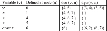
In general, it is difficult to carry out the type of analysis illustrated above for programs of non-trivial size. Usually test tools, such as χSUDS, automatically do such analysis and minimize the number of c- and p-uses to consider while generating tests to cover all c- and p-uses. Note that this analysis does not remove any c- and p-use from the program, it simply removes some of them from consideration because they are automatically covered by tests that cover some other c- and p-uses.
7.3.9 Data contexts and ordered data contexts
Let n be a node in a data flow graph. Each variable used at n is known as an input variable of n. Similarly, each variable defined at n is known as an output variable of n. The set of all live definitions of all input variables of node n is known as the data environment of node n and is denoted by DE(n).
A data environment is the set of all variables whose definitions are live at a node in a data flow graph.
Let X(n) = {x1, x2, ..., xk} be the set of input variables required for evaluation of any expression, arithmetic or otherwise, at node n in data flow graph F. Let ![]() denote the ijth definition of xj in F. An elementary data context of node n, denoted as EDC(n), is the set of definitions
denote the ijth definition of xj in F. An elementary data context of node n, denoted as EDC(n), is the set of definitions ![]() ik ≥ 1, of all variables in X(n) such that each definition is live when control arrives at node n. The data context of node n is the set of all its elementary data contexts and is denoted by DC(n). Given that the ijth definition of xj occurs at some node k, we shall refer to it as dk(xj).
ik ≥ 1, of all variables in X(n) such that each definition is live when control arrives at node n. The data context of node n is the set of all its elementary data contexts and is denoted by DC(n). Given that the ijth definition of xj occurs at some node k, we shall refer to it as dk(xj).
A data context is the set of all elementary data contexts for a node in a data flow graph.
Example 7.34 Let us examine node 4 in the data flow graph of Figure 7.7. The set of input variables of node 4, denoted by X(4), is {y, z}. The data environment for node 4, denoted by DE(4), is the set {d1(y), d6(y), d1(z), d4(z), d5(z)}.
Recall that each definition in DE(4) is live at node 4. For example, d4(z) is live at node 4 because there exists a path from the start of the program to node 4, and a path from node 4 back to node 4 without a redefinition of z until it has been used at node 4. This path is (1, 2, 3, 4, 6, 2, 3, 4). The first emphasized occurrence of node 4 is the one where z is defined and the second emphasized occurrence of node 4 is where this definition is live and used.
The data context DC(4) for node 4, and all other nodes in the graph, is given in the following table. Notice that the data context is defined only for nodes that contain at least one variable c-use. Thus, while determining data contexts, we exclude nodes that contain only a predicate. Nodes 1, 2, and 3 are three such nodes in Figure 7.7. Also, we have omitted some infeasible data contexts for node 6 (see Exercise 7.44).
Node k |
Data context DC(k) |
|---|---|
|
1 |
None |
|
2 |
None |
|
3 |
None |
|
4 |
{(d1(y), d1(z)), (d6(y), d4(z)), (d6(y), d5(z))} |
|
5 |
{(d1(z))} |
|
6 |
{ (d1(z), d1(y), d1(z), d1(count)), (d1(z), d1(y), d5(z), d1(count))), (d1(z), d1(y), d4(z), d1(count)), (d1(z), d6(y), d5(z), d6(count)), (d1(z), d6(y), d4(z), d6(count) )} |
|
7 |
{(d1(z)), (d4(z)), (d5(z))} |
The definitions of variables in an elementary data context occur along a program path in an order. For example, consider the elementary data context {d6(y), d4(z)} for node 4 in Figure 7.7. In the second occurrence of node 4 along the path (1, 2, 3, 4, 6, 2, 3, 4, 6, 7), d4(z) occurs first followed by d6(y). The sequence d6(z) followed by d6(y) is not feasible when control arrives at node 4. Hence only one sequence, i.e. d6(y) followed by d4(z), is possible for node 4.
Now consider the second occurrence of node 6 along the path (1, 2, 3, 6, 2, 5, 6, 7). The sequence of definitions of input variables of node 6 is d1(x) followed by d6(y), d6(count), and lastly d5(z). Next, consider again the second occurrence of node 6 but now along the path (1, 2, 5, 6, 2, 3, 6). In this case, the sequence of definitions is d1(x) followed by d5(z), d6(y), and lastly d6(count). These two sequences are different in that y and z are defined in a different sequence.
An ordered elementary data contexts imposes an ordering on the elements of an elementary data context. An ordered data context is the set of all elementary ordered data contexts.
The above examples lead to the notion of an ordered elementary data context of node n abbreviated as OEDC(n). An ordered elementary data context for node n in a data flow graph consists of a set of ordered sequence of definitions of the input variables of n. An ordered data context for node n is the set of all ordered elementary data contexts of node n denoted by ODC(n).
Example 7.35 Consider Program P7.17. The data flow graph for this program appears in Figure 7.8. The set of input variables for node 6 is {x, y}. The data context DC(6) for node 6 consists of four elementary data contexts given below.
DC(6)={d1(x), d1(y)), (d3(x), d1(y)), (d1(x), d4(y)), (d3(x), d4(y))} The ordered data context for the same node is given below.
ODC(6)= {(d1(x), d1(y)), (d1(y), d3(x)), (d1(x), d4(y)), (d3(x), d4(y)), (d4(y), d3(x))}
Notice that due to the inclusion of ordered elementary data contexts, ODC(6) has all items from DC(6) and one additional item that is not in DC(6).
Figure 7.8 Data flow graph of Program P7.17 to illustrate ordered data context.
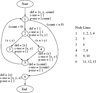
Program P7.17