1

Preliminaries: Software Testing

The purpose of this introductory chapter is to familiarize the reader with the basic concepts related to software testing. Here a framework is set up for the remainder of this book. Specific questions, answered in substantial detail in subsequent chapters, are raised here. After reading this chapter, you are likely to be able to ask meaningful questions related to software testing and reliability.

1.1  Humans, Errors, and Testing

Errors are a part of our daily life. Humans make errors in their thoughts, in their actions, and in the products that might result from their actions. Errors occur almost everywhere. For example, humans make errors in speech, in medical prescription, in surgery, in driving, in observation, in sports, and certainly in love and software development. Table 1.1 provides examples of human errors. The consequences of human errors vary significantly. An error might be insignificant in that it leads to a gentle friendly smile, such as when a slip of the tongue occurs. Or, an error may lead to a catastrophe, such as when an operator fails to recognize that a relief valve on the pressurizer was stuck open and this resulted in a disastrous radiation leak.

 

Table 1.1 Examples of errors in various fields of human endeavor.

Area	Error
Hearing	Spoken: He has a garage for repairing foreign cars. Heard: He has a garage for repairing falling cars.
Medicine	Incorrect antibiotic prescribed.
Music performance	Incorrect note played.
Numerical analysis	Incorrect algorithm for matrix inversion.
Observation	Operator fails to recognize that a relief valve is stuck open.
Software	Operator used: ≠, correct operator: >. Identifier used: new_line, correct identifier: next_line. Expression used: a∧(b∨c), correct expression: (a∧b)∨c. Data conversion from 64-bit floating point to 16-bit integer not protected (resulting in a software exception).
Speech	Spoken: waple malnut, intent: maple walnut. Spoken: We need a new refrigerator, intent: We need a new washing machine.
Sports	Incorrect call by the referee in a tennis match.
Writing	Written: What kind of pans did you use ? Intent: What kind of pants did you use ?

To determine whether there are any errors in our thought, actions, and the products generated, we resort to the process of testing. The primary goal of testing is to determine if the thoughts, actions, and products are as desired, that is, they conform to the requirements. Testing of thoughts is usually designed to determine if a concept or method has been understood satisfactorily. Testing of actions is designed to check if a skill that results in the actions has been acquired satisfactorily. Testing of a product is designed to check if the product behaves as desired. Note that both syntax and semantic errors arise during programming. Given that most modern compilers are able to detect syntactic errors, testing focuses on semantic errors, also known as faults, that cause the program under test to behave incorrectly.

 

Example 1.1   An instructor administers a test to determine how well the students have understood what the instructor wanted to convey. A tennis coach administers a test to determine how well the understudy makes a serve. A software developer tests the program developed to determine if it behaves as desired. In each of these three cases there is an attempt by a tester to determine if the human thoughts, actions, and products behave as desired. Behavior that deviates from the desirable is possibly due to an error.

 

Example 1.2   “Deviation from the expected” may not be due to an error for one or more reasons. Suppose that a tester wants to test a program to sort a sequence of integers. The program can sort an input sequence in both descending or ascending orders depending on the request made. Now suppose that the tester wants to check if the program sorts an input sequence in ascending order. To do so, she types in an input sequence and a request to sort the sequence in descending order. Suppose that the program is correct and produces an output that is the input sequence in descending order.

 

Upon examination of the output from the program, the tester hypothesizes that the sorting program is incorrect. This is a situation where the tester made a mistake (an error) that led to her incorrect interpretation (perception) of the behavior of the program (the product).

1.1.1  Errors, faults, and failures

There is no widely accepted and precise definition of the term “error.” Figure 1.1 illustrates one class of meanings for the terms error, fault, and failure. A programmer writes a program. An error occurs in the process of writing a program. A fault is the manifestation of one or more errors. A failure occurs when a faulty piece of code is executed leading to an incorrect state that propagates to the program’s output. The programmer might misinterpret the requirements and consequently write incorrect code. Upon execution, the program might display behavior that does not match with the expected behavior implying thereby that a failure has ocurred. A fault in the program is also commonly referred to as a bug or a defect. The terms error and bug are by far the most common ways of referring to something “wrong” in the program text that might lead to a failure. In this text, we often use the terms “error” and “fault” as synonyms. Faults are sometimes referred to as defects.

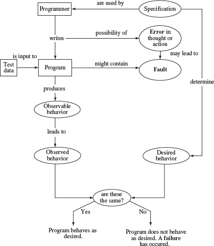
Figure 1.1 Errors, faults, and failures in the process of programming and testing.

In Figure 1.1, notice the separation of “observable” from “observed” behavior. This separation is important because it is the observed behavior that might lead one to conclude that a program has failed. Certainly, as explained earlier, this conclusion might be incorrect due to one or more reasons.

1.1.2  Test automation

Testing of complex systems, embedded and otherwise, can be a human intensive task. Often one needs to execute thousands of tests to ensure that, for example, a change made to a component of an application does not cause a previously correct code to malfunction. Execution of many tests can be tiring as well error prone. Hence, there is a tremendous need for automating testing tasks.

 

Most software development organizations automate test related tasks such as regression testing, GUI testing, and I/O device driver testing. Unfortunately the process of test automation cannot be generalized. For example, automating regression tests for an embedded device such as a pacemaker is quite different from that for an I/O device driver that connects to the USB port of a PC. Such lack of generalization often leads to specialized test automation tools developed in-house.

Nevertheless, there do exist general purpose tools for test automation. While such tools might not be applicable in all test environments, they are useful in many. Examples of such tools include Eggplant, Marathon, and Pounder for GUI testing; eLoadExpert, DBMonster, JMeter, Dieseltest, WAPT, LoadRunner, and Grinder for performance or load testing; and Echelon, TestTube, WinRunner, and XTest for regression testing. Despite the existence of a large number and a variety of test automation tools, large software-development organizations develop their own test automation tools primarily due to the unique nature of their test requirements.

AETG is an automated test generator that can be used in a variety of applications. It uses combinatorial design techniques, which we will discuss in Chapter 6. Random testing is often used for the estimation of reliability of products with respect to specific events. For example, one might test an application using randomly generated tests to determine how frequently does it crash or hang. DART is a tool for automatically extracting an interface of a program and generating random tests. While such tools are useful in some environments, they are dependent on the programming language used and the nature of the application interface. Therefore, many organizations develop their own tools for random testing.

1.1.3  Developer and tester as two roles

In the context of software engineering, a developer is one who writes code and a tester is one who tests code. We prefer to treat developer and tester as two distinct but complementary roles. Thus, the same individual could be a developer and a tester. It is hard to imagine an individual who assumes the role of a developer but never that of a tester, and vice versa. In fact, it is safe to assume that a developer assumes two roles, that of a “developer” and of a “tester,” though at different times. Similarly, a tester also assumes the same two roles but at different times.

 

Certainly, within a software development organization, the primary role of an individual might be to test and hence this individual assumes the role of a “tester.” Similarly, the primarily role of an individual who designs applications and writes code is that of a “developer.”

A reference to “tester” in this book refers to the role someone assumes when testing a program. Such an individual could be a developer testing a class she has coded, or a tester who is testing a fully-integrated set of components. A “programmer” in this book refers to an individual who engages in software development and often assumes the role of a tester, at least temporarily. This also implies that the contents of this book are valuable not only to those whose primary role is that of a tester, but also to those who work as developers.

1.2  Software Quality

We all want high-quality software. There exist several definitions of software quality. Also, one quality attribute might be more important to a user than another. In any case, software quality is a multidimensional quantity and is measurable. So, let us look at what defines the quality of a software.

1.2.1  Quality attributes

There exist several measures of software quality. These can be divided into static and dynamic quality attributes. Static quality attributes refer to the actual code and related documentation. Dynamic quality attributes relate to the behavior of the application while in use.

Static quality attributes include structured, maintainable, testable code as well as the availability of correct and complete documentation. You might have come across complaints such as “Product X is excellent, I like the features it offers, but its user manual stinks!” In this case, the user manual brings down the overall product quality. If you are a maintenance engineer and have been assigned the task of doing corrective maintenance on an application code, you will most likely need to understand portions of the code before you make any changes to it. This is where attributes such as code documentation, understandability, and structure come into play. A poorly-documented piece of code will be harder to understand and hence difficult to modify. Further, poorly-structured code might be harder to modify and difficult to test.

 

Dynamic quality attributes include software reliability, correctness, completeness, consistency, usability, and performance. Reliability refers to the probability of failure-free operation and is considered in the following section. Correctness refers to the correct operation of an application and is always with reference to some artifact. For a tester, correctness is with respect to the requirements; for a user, it is often with respect to a user manual.

 

Completeness refers to the availability of all features listed in the requirements, or in the user manual. An incomplete software is one that does not fully implement all features required. Of course, one usually encounters additional functionality with each new version of an application. This does not mean that a given version is incomplete because its next version has few new features. Completeness is defined with respect to a set of features that might itself be a subset of a larger set of features that are to be implemented in some future version of the application. Of course, one can easily argue that every piece of software that is correct is also complete with respect to some feature set.

 

Consistency refers to adherence to a common set of conventions and assumptions. For example, all buttons in the user interface might follow a common color coding convention. An example of inconsistency would be when a database application displays the date of birth of a person in the database; however, the date of birth is displayed in different formats, without any regard for the user’s preferences, depending on which feature of the database is used.

Usability refers to the ease with which an application can be used. This is an area in itself and there exist techniques for usability testing. Psychology plays an important role in the design of techniques for usability testing. Usability testing also refers to the testing of a product by its potential users. The development organization invites a selected set of potential users and asks them to test the product. Users in turn test for ease of use, functionality as expected, performance, safety, and security. Users thus serve as an important source of tests that developers or testers within the organization might not have conceived. Usability testing is sometimes referred to as user-centric testing.

Performance refers to the time the application takes to perform a requested task. Performance is considered as a non-functional requirement. It is specified in terms such as “This task must be performed at the rate of X units of activity in one second on a machine running at speed Y, having Z gigabytes of memory.” For example, the performance requirement for a compiler might be stated in terms of the minimum average time to compile of a set of numerical applications.

1.2.2  Reliability

People want software that functions correctly every time it is used. However, this happens rarely, if ever. Most softwares that are used today contain faults that cause them to fail on some combination of inputs. Thus, the notion of total correctness of a program is an ideal and applies mostly to academic and textbook programs.

 

Given that most software applications are defective, one would like to know how often a given piece of software might fail. This question can be answered, often with dubious accuracy, with the help of software reliability, hereafter referred to as reliability. There are several definitions of software reliability, a few are examined below.

 

1.3  Requirements, Behavior, and Correctness

Products, software in particular, are designed in response to requirements. Requirements specify the functions that a product is expected to perform. Once the product is ready, it is the requirements that determine the expected behavior. Of course, during the development of the product, the requirements might have changed from what was stated originally. Regardless of any change, the expected behavior of the product is determined by the tester’s understanding of the requirements during testing.

 

Example 1.3   Here are the two requirements, each of which leads to a different program.

 

Requirement 1:	It is required to write a program that inputs two integers and outputs the maximum of these.
Requirement 2:	It is required to write a program that inputs a sequence of integers and outputs the sorted version of this sequence.

Suppose that program max is developed to satisfy Requirement 1 above. The expected output of max when the input integers are 13 and 19, can be easily determined to be 19. Now suppose that the tester wants to know if the two integers are to be input to the program on one line followed by a carriage return, or on two separate lines with a carriage return typed in after each number. The requirement as stated above fails to provide an answer to this question. This example illustrates the incompleteness of Requirement 1.

The second requirement in the above example is ambiguous. It is not clear from this requirement whether the input sequence is to be sorted in ascending or descending order. The behavior of the sort program, written to satisfy this requirement, will depend on the decision taken by the programmer while writing sort.

Testers are often faced with incomplete and/or ambiguous requirements. In such situations, a tester may resort to a variety of ways to determine what behavior to expect from the program under test. For example, forth above program max, one way to determine how the input should be typed in is to actually examine the program text. Another way is to ask the developer of max as to what decision was taken regarding the sequence in which the inputs are to be typed in. Yet another method is to execute max on different input sequences and determine what is acceptable to max.

Regardless of the nature of the requirements, testing requires the determination of the expected behavior of the program under test. The observed behavior of the program is compared with the expected behavior to determine if the program functions as desired.

1.3.1  Input domain

A program is considered correct if it behaves as desired on all possible test inputs. Usually, the set of all possible inputs is too large for the program to be executed on each input. For example, suppose that the max program above is to be tested on a computer in which the integers range from –32,768 to 32,767. To test max on all possible integers would require it to be executed on all pairs of integers in this range. This will require a total of 2³² executions of max. It will take approximately 4.3 seconds to complete all executions assuming that testing is done on a computer that will take 1 nanosecond (=10^–9 seconds), to input a pair of integers, execute max, and check if the output is correct. Testing a program on all possible inputs is known as exhaustive testing.

 

A tester often needs to determine what constitutes “all possible inputs.” The first step in determining all possible inputs is to examine the requirements. If the requirements are complete and unambiguous, it should be possible to determine the set of all possible inputs. A definition is in order before we provide an example to illustrate how to determine the set of all program inputs.

 

Example 1.4   Using Requirement 1 from Example 1.3, we find the input domain of max to be the set of all pairs of integers where each element in the pair is in the range –32,768 till 32,767.

 

Example 1.5   Using Requirement 2 from Example 1.3, it is not possible to find the input domain for the sort program. Let us therefore assume that the requirement was modified to be the following:

 

Modified Requirement 2:

It is required to write a program that inputs a sequence of integers and outputs the integers in this sequence sorted in either ascending or descending order. The order of the output sequence is determined by an input request character that should be “A” when an ascending sequence is desired, and “D” otherwise. While providing input to the program, the request character is entered first followed by the sequence of integers to be sorted; the sequence is terminated with a period.

 

Based on the above modified requirement, the input domain for sort is a set of pairs. The first element of the pair is a character. The second element of the pair is a sequence of zero or more integers ending with a period. For example, following are three elements in the input domain of sort:

 

< A -3 15 12 55.>

< D 23 78.>

< A .>

 

The first element contains a sequence of four integers to be sorted in ascending order, the second element has a sequence to be sorted in descending order, and the third element has an empty sequence to be sorted in ascending order.

We are now ready to give the definition of program correctness.

 

1.3.2  Specifying program behavior

There are several ways to define and specify program behavior. The simplest way is to specify the behavior in a natural language such as English. However, this is more likely subject to multiple interpretations than a more formally specified behavior. Here, we explain how the notion of program “state” can be used to define program behavior and how the “state transition diagram,” or simply “state diagram,” can be used to specify program behavior.

 

The “state” of a program is the set of current values of all its variables and an indication of which statement in the program is to be executed next. One way to encode the state is by collecting the current values of program variables into a vector known as the “state vector.” An indication of where the control of execution is at any instant of time can be given by using an identifier associated with the next program statement. In the case of programs in assembly language, the location of control can be specified more precisely by giving the value of the program counter.

Each variable in the program corresponds to one element of this vector. Obviously, for a large program, such as the Unix operating system, the state vector might have thousands of elements. Execution of program statements causes the program to move from one state to the next. A sequence of program states is termed as program behavior.

 

Example 1.6   Consider a program that inputs two integers into variables X and Y, compares these values, sets the value of Ζ to the larger of the two, displays the value of Ζ on the screen, and exits. Program P1.1 shows the program skeleton. The state vector for this program consists of four elements. The first element is the statement identifier where the execution control is currently at. The next three elements are, respectively, the values of the three variables X, Y, and Z.

Program P1.1

1    integer X, Y, Z;

2    input (X, Y);

3    if (X < Y)

4       {Z=Y;}

5    else

6       {Z=X;}

7    endif

8    output (Z);

9    end

The letter u as an element of the state vector stands for an “undefined” value. The notation s_i → s_j is an abbreviation for “The program moves from state s_i to s_j.” The movement from s_i to s_j is caused by the execution of the statement whose identifier is listed as the first element of state s_i. A possible sequence of states that the max program may go through is given below.

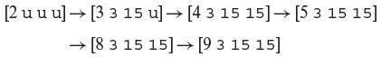
Upon the start of its execution, a program is in an “initial state.” A (correct) program terminates in its “final state.” All other program states are termed as “intermediate states.” In Example 1.6, the initial state is [2 u u u], the final state is [9 3 15 15], and there are four intermediate states as indicated.

 

Program behavior can be modeled as a sequence of states. With every program one can associate one or more states that need to be observed to decide whether or not the program behaves according to its requirements. In some applications it is only the final state that is of interest to the tester. In other applications a sequence of states might be of interest. More complex patterns might also be needed.

 

Example 1.7   For the max program (P1.1), the final state is sufficient to decide if the program has successfully determined the maximum of two integers. If the numbers input to max are 3 and 15, then the correct final state is [9 3 15 15]. In fact, it is only the last element of the state vector, 15, which may be of interest to the tester.

 

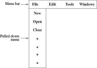
Example 1.8   Consider a menu-driven application named myapp. Figure 1.2 shows the menu bar for this application. It allows a user to position and click the mouse on any one of a list of menu items displayed in the menu bar on the screen. This results in the “pulling down” of the menu and a list of options is displayed on the screen. One of the items on the menu bar is labeled File. When File is pulled down, it displays Open as one of several options. When the Open option is selected, by moving the cursor over it, it should be highlighted. When the mouse is released, indicating that the selection is complete, a window displaying names of files in the current directory should be displayed.

Figure 1.2 Menu bar displaying four menu items when application myapp is started.

Figure 1.3 depicts the sequence of states that myapp is expected to enter when the user actions described above are performed. When started, the application enters the initial state wherein it displays the menu bar and waits for the user to select a menu item. This state diagram depicts the expected behavior of myapp in terms of a state sequence. As shown in Figure 1.3, myapp moves from state s₀ to state s₃ after the sequence of actions t₀, t₁, t₂, and t₃ has been applied. To test myapp, the tester could apply the sequence of actions depicted in this state diagram and observe if the application enters the expected states.

Figure 1.3 A state sequence for myapp showing how the application is expected to behave when the user selects the open option under the File menu item.

 

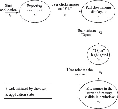
As you might observe from Figure 1.3, a state sequence diagram can be used to specify the behavioral requirements of an application. This same specification can then be used during testing to ensure if the application conforms to the requirements.

1.3.3  Valid and invalid inputs

In the examples above, the input domains are derived from the requirements. However, due to the incompleteness of requirements, one might have to think a bit harder to determine the input domain. To illustrate why, consider the modified requirement in Example 1.5. The requirement mentions that the request characters can be “A” or “D”, but it fails to answer the question “What if the user types a different character ?” When using sort it is certainly possible for the user to type a character other than “A” or “D”. Any character other than “A” or “D” is considered as invalid input to sort. The requirement for sort does not specify what action it should take when an invalid input is encountered.

 

Identifying the set of invalid inputs and testing, the program against these inputs is an important part of the testing activity. Even when the requirements fail to specify the program behavior on invalid inputs, the programmer does treat these in one way or another. Testing a program against invalid inputs might reveal errors in the program.

 

Example 1.9   Suppose that we are testing the sort program. We execute it against the following input: < Ε 7 19 . >. The requirements in Example 1.5 are insufficient to determine the expected behavior of sort on the above input. Now suppose that upon execution on the above input, the sort program enters into an infinite loop and neither asks the user for any input nor responds to anything typed by the user. This observed behavior points to a possible error in sort.

The argument above can be extended to apply to the sequence of integers to be sorted. The requirements for the sort program do not specify how the program should behave if, instead of typing an integer, a user types in a character, such as “?”. Of course, one would say, the program should inform the user that the input is invalid. But this expected behavior from sort needs to be tested. This suggests that the input domain for sort should be modified.

 

Example 1.10   Considering that sort may receive valid and invalid inputs, the input domain derived in Example 1.5 needs modification. The modified input domain consists of pairs of values. The first value in the pair is any ASCII character that can be typed by a user as a request character. The second element of the pair is a sequence of integers, interspersed with invalid characters, terminated by a period. Thus, for example, the following are sample elements from the modified input domain:

 

< A 7 19.>

< D 7 9F 19.>

 

In the example above, we assumed that invalid characters are possible inputs to the sort program. This, however, may not be the case in all situations. For example, it might be possible to guarantee that the inputs to sort will always be correct as determined from the modified requirements in Example 1.5. In such a situation, the input domain need not be augmented to account for invalid inputs if the guarantee is to be believed by the tester.

In cases where the input to a program is not guaranteed to be correct, it is convenient to partition the input domain into two subdomains. One subdomain consists of inputs that are valid and the other consists of inputs that are invalid. A tester can then test the program on selected inputs from each subdomain.

1.4  Correctness Versus Reliability

1.4.1  Correctness

Though correctness of a program is desirable, it is almost never the objective of testing. To establish correctness via testing would imply testing a program on all elements in the input domain. In most cases that are encountered in practice, this is impossible to accomplish. Thus, correctness is established via mathematical proofs of programs. A proof uses the formal specification of requirements and the program text to prove or disprove that the program will behave as intended. While a mathematical proof is precise, it too is subject to human errors. Even when the proof is carried out by a computer, the simplification of requirements specification and errors in tasks that are not fully automated might render the proof useless.

 

While correctness attempts to establish that the program is error free, testing attempts to find if there are any errors in it. Completeness of testing does not necessarily demonstrate that a program is error free. However, as testing progresses, errors might be revealed. Removal of errors from the program usually improves the chances, or the probability, of the program executing without any failure. Also, testing, debugging, and the error removal processes together increase our confidence in the correct functioning of the program under test.

 

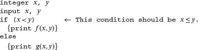
Example 1.11   This example illustrates why the probability of program failure might not change upon error removal. Consider the following program that inputs two integers x and y and prints the value of f (x, y) or g(x, y) depending on the condition x < y.

The above program uses two functions f and g not defined here. Let us suppose that function f produces an incorrect result whenever it is invoked with x = y and that f (x, y) ≠ g(x, y), x = y. In its present form, the program fails when tested with equal input values because function g is invoked instead of function f. When the error is removed by changing the condition x < y to x ≤ y, the program fails again when the input values are the same. The latter failure is due to the error in function f. In this program, when the error in f is also removed, the program will be correct assuming that all other code is correct.

1.4.2  Reliability

The probability of a program failure is captured more formally in the term “reliability.” Consider the second of the two definitions examined earlier: “The reliability of a program Ρ is the probability of its successful execution on a randomly selected element from its input domain.”

 

A comparison of program correctness and reliability reveals that while correctness is a binary metric, reliability is a continuous metric over a scale from 0 to 1. A program can be either correct or incorrect; its reliability can be anywhere between 0 and 1. Intuitively, when an error is removed from a program, the reliability of the program so obtained is expected to be higher than that of the one that contains the error. As illustrated in the example above, this may not be always true. The next example illustrates how to compute program reliability in a simplistic manner.

 

Example 1.12   Consider a program Ρ that takes a pair of integers as input. The input domain of this program is the set of all pairs of integers. Suppose now that in actual use there are only three pairs that will be input to P. These are

 

{<(0, 0) (–l, l) (l, –l)>}

 

The above set of three pairs is a subset of the input domain of Ρ and is derived from a knowledge of the actual use of P, and not solely from its requirements.

Suppose also that each pair in the above set is equally likely to occur in practice. If it is known that Ρ fails on exactly one of the three possible input pairs then the frequency with which Ρ will function correctly is This number is an estimate of the probability of the successful operation of Ρ and hence is the reliability of P.

1.4.3  Operational profiles

As per the definition above, the reliability of a program depends on how it is used. Thus, in Example 1.12, if Ρ is never executed on input pair (0, 0), then the restricted input domain becomes {< (–1, 1) (1, –1) >} and the reliability of Ρ is 1. This leads us to the definition of operational profile.

 

Example 1.13   Consider a sort program that, on any given execution, allows any one of two types of input sequences. One sequence consists of numbers only and the other consists of alphanumeric strings. One operational profile for sort is specified as follows:

Operational profile #1
Sequence	Probability
Numbers only	0.9
Alphanumeric strings	0.1

Another operational profile for sort is specified as follows:

Operational profile #2
Sequence	Probability
Numbers only	0.1
Alphanumeric strings	0.9

The two operational profiles above suggest significantly different uses of sort. In one case, it is used mostly for sorting sequences of numbers, and in the other case, it is used mostly for sorting alphanumeric strings.

1.5  Testing and Debugging

Testing is the process of determining if a program behaves as expected. In the process, one may discover errors in the program under test. However, when testing reveals an error, the process used to determine the cause of this error and to remove it is known as debugging. As illustrated in Figure 1.4, testing and debugging are often used as two related activities in a cyclic manner.

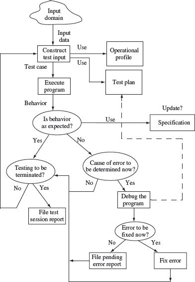
Figure 1.4 A test and debug cycle.

1.5.1  Preparing a test plan

A test cycle is often guided by a test plan. When relatively small programs are being tested, a test plan is usually informal and in the tester’s mind, or there may be no plan at all. A sample test plan for testing the sort program is shown in Figure 1.5.

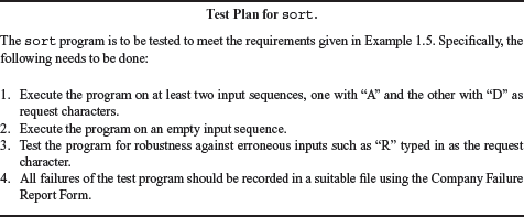
Figure 1.5 A sample test plan for the sort program.

The sample test plan in Figure 1.5 is often augmented by items such as the method used for testing, method for evaluating the adequacy of test cases, and method to determine if a program has failed or not.

1.5.2  Constructing test data

A test case is a pair of input data and the corresponding program output. The test data are a set of values: one for each input variable. A test set is a collection of test cases. A test set is sometimes referred to as a test suite. The notion of “one execution” of a program is rather tricky and is elaborated later in this chapter. Test data is an alternate term for test set.

 

Program requirements and the test plan help in the construction of test data. Execution of the program on test data might begin after all or a few test cases have been constructed. While testing, relatively small programs testers often generate a few test cases and execute the program against these. Based on the results obtained, the tester decides whether to continue the construction of additional test cases or to enter the debugging phase.

 

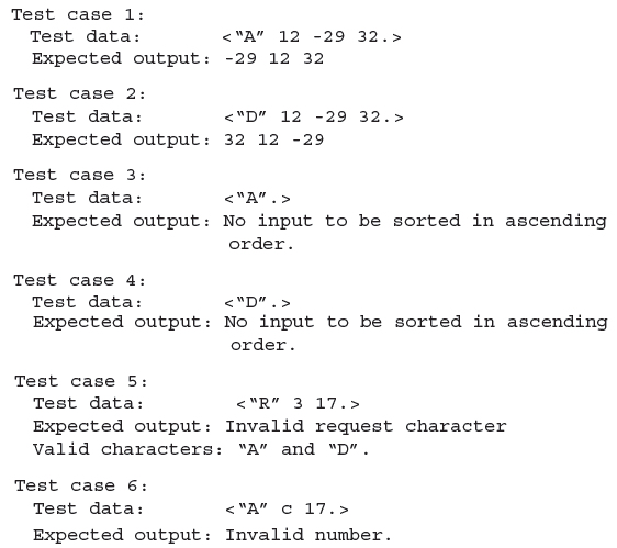
Example 1.14   The following test cases are generated for the sort program using the test plan in Figure 1.5. 

Test cases 1 and 2 are derived in response to item 1 in the test plan; 3 and 4 are in response to item 2. Notice that we have designed two test cases in response to item 2 of the test plan even though the plan calls for only 1 test case. Notice also that the requirements for the sort program as in Example 1.5 do not indicate what should be the output of sort when there is nothing to be sorted. We therefore took an arbitrary decision while composing the “Expected output” for an input that has no numbers to be sorted. Test cases 5 and 6 are in response to item 3 in the test plan.

 

As is evident from the above example, one can select a variety of test sets to satisfy the test plan requirements. Questions such as “Which test set is the best?” and “Is a given test set adequate?” are answered in Part III of this book.

1.5.3  Executing the program

Execution of a program under test is the next significant step in testing. Execution of this step for the sort program is most likely a trivial exercise. However, this may not be so for large and complex programs. For example, to execute a program that controls a digital cross connect switch used in telephone networks, one may first need to follow an elaborate procedure to load the program into the switch and then yet another procedure to input the test cases to the program. Obviously, the complexity of actual program execution is dependent on the program itself.

 

Often a tester might be able to construct a test harness to aid in program execution. The harness initializes any global variables, inputs a test case, and executes the program. The output generated by the program may be saved in a file for subsequent examination by a tester. The next example illustrates a simple test harness.

 

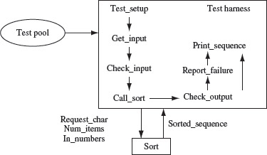
Example 1.15   The test harness in Figure 1.6 reads an input sequence, checks for its correctness, and then calls sort. The sorted array sorted_sequence returned by sort is printed using the print_sequence procedure. Test cases are assumed to be available in the Test pool file shown in the figure. In some cases, the tests might be generated from within the harness.

Figure 1.6 A simple test harness to test the sort program.

In preparing this test harness we assume that (a) sort is coded as a procedure, (b) the get_input procedure reads the request character and the sequence to be sorted into variables request_char, num_items, and in_numbers, and (c) the input is checked prior to calling sort by the check_input procedure.

The test_setup procedure is usually invoked first to set up the test that, in this example, includes identifying and opening the file containing tests. The check_output procedure serves as the oracle that checks if the program under test behaves correctly. The report_failure procedure is invoked in case the output from sort is incorrect. A failure might be simply reported via a message on the screen or saved in a test report file (not shown in Figure 1.6). The print_sequence procedure prints the sequence generated by the sort program. The output generated by print_sequence can also be piped into a file for subsequent examination.

1.5.4  Assessing program correctness

An important step in testing a program is the one wherein the tester determines if the observed behavior of the program under test is correct or not. This step can be further divided into two smaller steps. In the first step one observes the behavior and in the second step analyses the observed behavior to check if it is correct or not. Both these steps can be trivial for small programs, such as for max in Example 1.3, or extremely complex as in the case of a large distributed software system. The entity that performs the task of checking the correctness of the observed behavior is known as an oracle. Figure 1.7 shows the relationship between the program under test and the oracle.

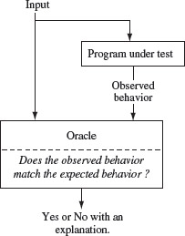
Figure 1.7 Relationship between the program under test and the oracle. The output from an oracle can be binary such as “Yes” or “No” or more complex such as an explanation as to why the oracle finds the observed behavior to be same or different from the expected behavior.

A tester often assumes the role of an oracle and thus serves as a “human oracle.” For example, to verify if the output of a matrix multiplication program is correct or not, a tester might input two 2 × 2 matrices and check if the output produced by the program matches the results of hand calculation. As another example, consider checking the output of a text processing program. In this case, a human oracle might visually inspect the monitor screen to verify whether or not the italicize command works correctly when applied to a block of text.

 

Checking program behavior by humans has several disadvantages. First, it is error prone as the human oracle might make an error in analysis. Second, it may be slower than the speed with which the program computed the results. Third, it might result in the checking of only trivial input–output behaviors. However, regardless of these disadvantages, a human oracle can often be the best available oracle.

Oracles can also be programs designed to check the behavior of other programs. For example, one might use a matrix multiplication program to check if a matrix inversion program has produced the correct output. In this case, the matrix inversion program inverts a given matrix A and generates Β as the output matrix. The multiplication program can check to see if Α × Β = I within some bounds on the elements of the identity matrix I. Another example is an oracle that checks the validity of the output from a sort program. Assuming that the sort program sorts input numbers in ascending order, the oracle needs to check if the output of the sort program is indeed in ascending order.

Using programs as oracles has the advantage of speed, accuracy, and the ease with which complex computations can be checked. Thus, a matrix multiplication program, when used as an oracle for a matrix inversion program, can be faster, accurate, and check very large matrices when compared to the same function performed by a human oracle.

1.5.5  Constructing an oracle

Construction of an automated oracle, such as the one to check a matrix multiplication or a sort program, requires the determination of input–output relationship. For matrix inversion, and for sorting, this relation is rather simple and expressed precisely in terms of a mathematical formula or a simple algorithm as explained above. Also, when tests are generated from models such as finite state machines or statecharts, both inputs and the corresponding outputs are available. This makes it possible to construct an oracle while generating the tests. However, in general, the construction of an automated oracle is a complex undertaking. The next example illustrates one method for constructing an oracle.

 

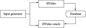
Example 1.16   Consider a program named HVideo that allows one to keep track of old home videos. The program operates in two modes: data entry and search. In the date entry mode, it displays a screen into which the user types in information about a video cassette. This information includes data such as the title, the comments, and the date when the video was prepared. Once the information is typed the user clicks on the Enter button, which results in this information being added to a database. In the search mode, the program displays a screen into which a user can type some attribute of the video being searched for and sets up a search criterion. A sample criterion is “Find all videos that contain the name Sonia in the title field.” In response, the program returns all videos in the database that match the search criteria or displays an appropriate message if no match is found.

To test HVideo, we need to create an oracle that checks whether or not the program functions correctly in data entry and search modes. In addition, an input generator needs to be created. As shown in Figure 1.8, the input generator generates inputs for HVideo. To test the data entry operation of HVideo, the input generator generates a data entry request. This request consists of an operation code, Data Entry, and the data to be entered that includes the title, the comments, and the date on which the video was prepared. Upon completion of execution of the Enter request, HVideo returns control to the input generator. The input generator now requests the oracle to test if HVideo performed its task correctly on the input given for data entry. The oracle uses the input to check if the information to be entered into the database has been entered correctly or not. The oracle returns a Pass or No Pass to the input generator.

Figure 1.8 Relationship between an input generator, HVideo, and its oracle.

To test if HVideo correctly performs the search operation, the input generator formulates a search request with the search data the same as the one given previously with the Enter command. This input is passed on to HVideo that performs the search and returns the results of the search to the input generator. The input generator passes these results to the oracle to check for their correctness. There are at least two ways in which the oracle can check for the correctness of the search results. One is for the oracle to actually search the database. If its findings are the same as that of HVideo, then the search results are assumed to be correct and incorrect otherwise.

1.6  Test Metrics

The term “metric” refers to a standard of measurement. In software testing, there exist a variety of metrics. Figure 1.9 shows a classification of various types of metrics briefly discussed in this section. Metrics can be computed at the organizational, process, project, and product levels. Each set of measurements has its value in monitoring, planning, and control.

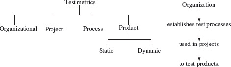
Figure 1.9 Types of metrics used in software testing and their relationships.

Regardless of the level at which metrics are defined and collected, there exist four general core areas that assist in the design of metrics. These are schedule, quality, resources, and size. Schedule-related metrics measure actual completion times of various activities and compare these with estimated time to completion. Quality-related metrics measure the quality of a product or a process. Resource-related metrics measure items such as cost in dollars, manpower, and tests executed. Size-related metrics measure the size of various objects such as the source code and the number of tests in a test suite.

1.6.1  Organizational metrics

Metrics at the level of an organization are useful in overall project planning and management. Some of these metrics are obtained by aggregating compatible metrics across multiple projects. Thus, for example, the number of defects reported after product release, averaged over a set of products developed and marketed by an organization, is a useful metric of product quality at the organizational level.

Computing this metric at regular intervals and overall products released over a given duration shows the quality trend across the organization. For example, one might say “The number of defects reported in the field over all products and within three months of their shipping, has dropped from 0.2 defects per KLOC (thousand lines of code) to 0.04 defects KLOC.” Other organizational level metrics include testing cost per KLOC, delivery schedule slippage, and time to complete system testing.

 

Organizational level metrics allow senior management to monitor the overall strength of the organization and points to areas of weaknesses. These metrics help the senior management in setting new goals and plan for resources needed to realize these goals.

 

Example 1.17   The average defect density across all software projects in a company is 1.73 defects per KLOC. Senior management has found that for the next generation of software products, which they plan to bid, they need to show that product density can be reduced to 0.1 defects per KLOC. The management thus sets a new goal.

Given the time frame from now until the time to bid, the management needs to do a feasibility analysis to determine whether or not this goal can be met. If a preliminary analysis shows that it can be met, then a detailed plan needs to be worked out and put into action. For example, management might decide to train its employees in the use of new tools and techniques for defect prevention and detection using sophisticated static analysis techniques.

1.6.2  Project metrics

Project metrics relate to a specific project, for example, the I/O device testing project or a compiler project. These are useful in the monitoring and control of a specific project. The ratio of actual to planned system test effort is one project metric. Test effort could be measured in terms of the tester-man-months. At the start of the system test phase, for example, the project manager estimates the total system test effort. The ratio of actual to estimated effort is zero prior to the system test phase. This ratio builds up over time. Tracking the ratio assists the project manager in allocating testing resources.

Another project metric is the ratio of the number of successful tests to the total number of tests in the system test phase. At any time during the project, the evolution of this ratio from the start of the project could be used to estimate the time remaining to complete the system test process.

1.6.3  Process metrics

Every project uses some test process. The “big bang” approach is one process sometimes used in relatively small single person projects. Several other well-organized processes exist. The goal of a process metric is to assess the “goodness” of the process.

When a test process consists of several phases, for example, unit test, integration test, system test, etc, one can measure how many defects were found in each phase. It is well known that the later a defect is found, the costlier it is to fix. Hence, a metric that classifies defects according to the phase in which they are found assists in evaluating the process itself.

 

Example 1.18   In one software development project, it was found that 15% of the total defects were reported by customers, 55% of the defects prior to shipping were found during system test, 22% during integration test, and the remaining during unit test. The large number of defects found during the system test phase indicates a possibly weak integration and unit test process. The management might also want to reduce the fraction of defects reported by customers.

1.6.4  Product metrics: generic

Product metrics relate to a specific product such as a compiler for a programming language. These are useful in making decisions related to the product, for example, “Should this product be released for use by the customer ?”

Product quality-related metrics abound. We introduce two types of metrics here: the cyclomatic complexity and the Halstead metrics. The cyclomatic complexity proposed by Thomas McCabe in 1976 is based on the control flow of a program. Given the CFG G (see Chapter 2.2 for details) of program Ρ containing Ν nodes, Ε edges, and p connected procedures, the cyclomatic complexity V(G) is computed as follows:

 

 

Note that Ρ might consist of more than one procedure. The term p in V(G) counts only procedures that are reachable from the main function. V(G) is the complexity of a CFG G that corresponds to a procedure reachable from the main procedure. Also, V(G) is not the complexity of the entire program, instead it is the complexity of a procedure in Ρ that corresponds to G (see Exercise 1.12). Larger values of V(G) tend to imply higher program complexity and hence a program more difficult to understand and test than one with a smaller values. V(G) is 5 or less are recommended.

The now well-known Halstead complexity measures were published by late Professor Maurice Halstead in a book titled “Elements of Software Science.” Table 1.2 lists some of the software science metrics. Using program size (S) and effort (E), the following estimator has been proposed for the number of errors (B) found during a software development effort:

 

Extensive empirical studies have been reported to validate Halstead’s software science metrics. An advantage of using an estimator such as Β is that it allows the management to plan for testing resources. For example, a larger value of the number of expected errors will lead to a larger number of testers and testing resources to complete the test process over a given duration. Nevertheless, modern programming languages such as Java and C++ do not lend themselves well to the application of the software science metrics. Instead, one uses specially devised metrics for object-oriented languages described next (also see Exercise 1.16).

 

Table 1.2 Halstead measures of program complexity and effort.

Measure	Notation	Definition
Operator count	N1	Number of operators in a program
Operand count	N2	Number of operands in a program.
Unique operators	η1	Number of unique operators in a program
Unique operands	η2	Number of unique operands in a program
Program vocabulary	η	η1 + η2
Program size	N	N1 + N2
Program volume	V	N × log2η
Difficulty	D	2/η1 × η2/N2
Effort	E	D × V

1.6.5  Product metrics: OO software

A number of empirical studies have investigated the correlation between product complexity metric application quality. Table 1.3 lists a sample of product metrics for object-oriented and other applications. Product reliability is a quality metric and refers to the probability of product failure for a given operational profile. As explained in Section 1.4.2, product reliability of software truly measures the probability of generating a failure causing test input. If for a given operational profile and in a given environment this probability is 0, then the program is perfectly reliable despite the possible presence of errors. Certainly, one could define other metrics to assess software reliability. A number of other product quality metrics, based on defects, are listed in Table 1.3.

 

Table 1.3 A sample of product metrics.

Metric	Meaning
Reliability   Defects density Defect severity Test coverage	Probability of failure of a software product with respect to a given operational profile in a given environment. Number of defects per KLOC. Distribution of defects by their level of severity Fraction of testable items, e.g., basic blocks, covered. Also, a metric for test adequacy or "goodness of tests."
Cyclomatic complexity Weighted methods per class Class coupling Response set Number of children	Measures complexity of a program based on its CFG. , where ci is the complexity of method i in the class under consideration. Measures the number of classes to which a given class is coupled. Set of all methods that can be invoked, directly and indirectly, when a message is sent to object O. Number of immediate descendants of a class in the class hierarchy.

The OO metrics in the table are due to Shyam Chidamber and Chris Kemerer. They measure program or design complexity. They are of direct relevance to testing in that a product with a complex design will likely require more test effort to obtain a given level of defect density than a product with less complexity.

1.6.6  Progress monitoring and trends

Metrics are often used for monitoring progress. This requires making measurements on a regular basis over time. Such measurements offer trends. For example, suppose that a browser has been coded, unit tested, and its components integrated. It is now in the system testing phase. One could measure the cumulative number of defects found and plot these over time. Such a plot will rise over time. Eventually, it will likely show a saturation indicating that the product is reaching a stability stage. Figure 1.10 shows a sample plot of new defects found over time.

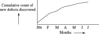
Figure 1.10 A sample plot of cumulative count of defects found over seven consecutive months in a software project.

1.6.7  Static and dynamic metrics

Static metrics are those computed without having to execute the product. Number of testable entities in an application is an example of a static product metric. Dynamic metrics require code execution. For example, the number of testable entities actually covered by a test suite is a dynamic product metric.

 

One could apply the notions of static and dynamic metrics to organization and project. For example, the average number of testers working on a project is a static project metric. Number of defects remaining to be fixed could be treated as a dynamic metric as it can be computed accurately only after a code change has been made and the product retested.

1.6.8  Testability

According to IEEE, testability is the “degree to which a system or component facilitates the establishment of test criteria and the performance of tests to determine whether those criteria have been met.” Different ways to measure testability of a product can be categorized into static and dynamic testability metrics. Software complexity is one static testability metric. The more complex an application, the lower the testability, that is, the higher the effort required to test it. Dynamic metrics for testability include various code-based coverage criteria. For example, a program for which it is difficult to generate tests that satisfy the statement coverage criterion is considered to have low testability than one for which it is easier to construct such tests.

 

High testability is a desirable goal. This is done best by knowing what needs to be tested and how, well in advance. It is recommended that features to be tested and how they are to be tested must be identified during the requirements stage. This information is then updated during the design phase and carried over to the coding phase. A testability requirement might be met through the addition of some code to a class. In more complex situations, it might require special hardware and probes in addition to special features aimed solely at meeting a testability requirement.

 

Example 1.19   Consider an application Ε required to control the operation of an elevator. Ε must pass a variety of tests. It must also allow a tester to perform a variety of tests. One test checks if the elevator hoists motor and the brakes are working correctly. Certainly one could do this test when the hardware is available. However, for concurrent hardware and software development, one needs a simulator for the hoist motor and brake system.

To improve the testability of E, one must include a component that allows it to communicate with a hoist motor and brake simulator and display the status of the simulated hardware devices. This component must also allow a tester to input tests such as “start the motor.”

Another test requirement for E is that it must allow a tester to experiment with various scheduling algorithms. This requirement can be met by adding a component to Ε that offers a palette of scheduling algorithms to choose from and whether or not they have been implemented. The tester selects an implemented algorithm and views the elevator movement in response to different requests. Such testing also requires a “random request generator” and a display of such requests and the elevator response (also see Exercise 1.14).

 

Testability is a concern in both hardware and software designs. In hardware design, testability implies that there exist tests to detect any fault with respect to a fault model in a finished product. Thus, the aim is to verify the correctness of a finished product. Testability in software focuses on the verification of design and implementation.

1.7  Software and Hardware Testing

There are several similarities and differences between techniques used for testing software and hardware. It is obvious that a software application does not degrade over time, any fault present in the application will remain, and no new faults will creep in unless the application is changed. This is not true for hardware, such as a VLSI chip, that might fail over time due to a fault that did not exist at the time the chip was manufactured and tested.

This difference in the development of faults during manufacturing or over time leads to built-in self test (BIST) techniques applied to hardware designs and rarely, if at all, to software designs and code. BIST can be applied to software but will only detect faults that were present when the last change was made. Note that internal monitoring mechanisms often installed in software are different from BIST intended to actually test or the correct functioning of a circuit.

Fault models: Hardware testers generate tests based on fault models. For example, using a stuck-at fault model a set of input test patterns can be used to test whether or not a logic gate is functioning as expected. The fault being tested for is a manufacturing flaw or might have developed due to degradation over time. Software testers generate tests to test for correct functionality. Sometimes such tests do not correspond to any general fault model. For example, to test whether or not there is a memory leak in an application, one performs a combination of stress testing and code inspection. A variety of faults could lead to memory leaks.

Hardware testers use a variety of fault models at different levels of abstraction. For example, at the lower level there are transistor level faults. At higher levels there are gate level, circuit level, and function level fault models. Software testers might or might not use fault models during test generation even though the models exist. Mutation testing described in Chapter 8 is a technique based on software fault models. Other techniques for test generation such as condition testing, finite state model-based testing, and combinatorial designs are also based on well-defined fault models which shall be discussed in Chapters 4–6, respectively. Techniques for automatic generation of tests, as described in several chapters in Part II of this book are based on precise fault models.

Test domain: A major difference between tests for hardware and software is in the domain of tests. Tests for a VLSI chip, for example, take the form of a bit pattern. For combinational circuits, for example, a multiplexer, a finite set of bit patterns will ensure the detection of any fault with respect to a circuit level fault model. For sequential circuits that use flip-flops, a test may be a sequence of bit patterns that move the circuit from one state to another and a test suite is a collection of such tests. For software, the domain of a test input is different than that for hardware. Even for the simplest of programs, the domain could be an infinite set of tuples with each tuple consisting of one or more basic data types such as integers and reals.

 

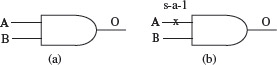
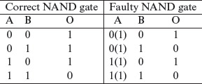
Example 1.20   Consider a simple 2-input NAND gate in Figure 1.11(a). The stuck-at fault model defines several faults at the input and output of a logic gate. Figure 1.11(b) shows a 2-input NAND gate with a stuck-at-1 fault, abbreviated as s-a-1, at input A. The truth tables for the correct and the faulty NAND gates are shown below.

Figure 1.11 (a) A 2-input NAND gate, (b) A NAND gate with a stuck-at 1 fault in input A.

 

Stuck-at fault models are common in hardware.

A test bit vector v: (A = 0, Β = 1) leads to output 0 whereas the correct output should be 1. Thus, v detects a single s-a-1 fault in the A input of the NAND gate. There could be multiple stuck-at faults. Exercise 1.15 asks you to determine whether or not multiple stuck-at faults in a 2-input NAND gate can always be detected.

 

Test coverage: It is practically impossible to completely test a large piece of software, for example, an operating system as well as a complex integrated circuit such as a modern 32 or 64-bit microprocessor. This leads to the notion of acceptable test coverage. In VLSI testing, such coverage is measured using a fraction of the faults covered to the total that might be present with respect to a given fault model.

The idea of fault coverage in hardware is also used in software testing using program mutation. A program is mutated by injecting a number of faults using a fault model that corresponds to mutation operators. The adequacy of a test set is assessed as a fraction of the mutants covered to the total number mutants. Details of this technique are described in Chapter 8.

Test set efficiency: There are multiple definitions of test set efficiency. Here we give one. Let T be a test set developed to test program P that must meet requirements R. Let f be the number of faults in Ρ and f′ the number faults detected when Ρ is executed against test cases in Τ. The efficiency of Τ is measured as the ratio Note that the efficiency is a number between 0 and 1. This definition of test set efficiency is also referred to as the effectiveness of a test set.

In most practical situations, one would not know the number of faults in a program under test. Hence, in such situations it is not possible to measure precisely the efficiency of a test set. Nevertheless, empirical studies are generally used to measure the efficiency of a test set by using well-known and understandable programs that are seeded with known faults.

Note that the size of a test set is not accounted for in the above definition of efficiency. However, given two test sets with equal efficiency, it is easy to argue that one would prefer to use the one that contains fewer tests.

The term test efficiency is different from test set or test suite efficiency. While the latter refers to the efficiency of a test suite, test efficiency refers to the efficiency of the test process. The efficiency of a test process is often defined as follows: Let D denote the total number of defects found during the various phases of testing excluding the user acceptance phase. Let D_u be the number of defects found in user acceptance testing and D′ = D + D_u. Then, test efficiency is defined as

Notice that test suite efficiency and test efficiency are two quite different metrics. Test set efficiency is an indicator of the goodness of the techniques used to develop the tests. Test efficiency is an indicator of the goodness of the entire test process, and hence it includes in some ways, test set metrics.

1.8  Testing and Verification

Program verification aims at proving the correctness of programs by showing that it contains no errors. This is very different from testing that aims at uncovering errors in a program. While verification aims at showing that a given program works for all possible inputs that satisfy a set of conditions, testing aims to show that the given program is reliable in that no errors of any significance were found.

 

Program verification and testing are best considered as complementary techniques. In practice, one often sheds program verification, but not testing. However, in the development of critical applications, such as smart cards, or control of nuclear plants, one often makes use of verification techniques to prove the correctness of some artifact created during the development cycle, not necessarily the complete program. Regardless of such proofs, testing is used invariably to obtain confidence in the correctness of the application.

Testing is not a perfect process in that a program might contain errors despite the success of a set of tests. However, it is a process with direct impact on our confidence in the correctness of the application under test. Our confidence in the correctness of an application increases when an application passes a set of thoroughly designed and executed tests.

Verification might appear to be a perfect process as it promises to verify that a program is free from errors. However, a close look at verification reveals that it has its own weaknesses. The person who verified a program might have made mistakes in the verification process; there might be an incorrect assumption on the input conditions; incorrect assumptions might be made regarding the components that interface with the program, and so on. Thus, neither verification nor testing are perfect techniques for proving the correctness of programs.

It is often stated that programs are mathematical objects and must be verified using mathematical techniques of theorem proving. While one could treat a program as a mathematical object, one must also realize the tremendous complexity of this object that exists within the program and also in the environment in which it operates. It is this complexity that has prevented formal verification of programs such as the 5ESS switch software from AT&T, the various versions of the Windows operating system, and other monstrously complex programs. Of course, we all know that these programs are defective, but the fact remains that they are usable and provide value to users.

1.9  Defect Management

Defect management is an integral part of a development and test process in many software development organizations. It is a subprocess of the development process. It entails the following: defect prevention, discovery, recording and reporting, classification, resolution, and prediction.

 

Defect prevention is achieved through a variety of processes and tools. For example, good coding techniques, unit test plans, and code inspections are all important elements of any defect prevention process. Defect discovery is the identification of defects in response to failures observed during dynamic testing or found during static testing. Discovering a defect often involves debugging the code under test.

Defects found are classified and recorded in a database. Classification becomes important in dealing with the defects. For example, defects classified as “high severity” will likely be attended to first by the developers than those classified as “low severity.” A variety of defect classification schemes exist. Orthogonal defect classification, popularly known as ODC, is one such scheme. Defect classification assists an organization in measuring statistics such as the types of defects, their frequency, and their location in the development phase and document. These statistics are then input to the organization’s process improvement team that analyzes the data, identifies areas of improvement in the development process, and recommends appropriate actions to higher management.

Each defect, when recorded, is marked as “open” indicating that it needs to be resolved. One or more developers are assigned to resolve the defect. Resolution requires careful scrutiny of the defect, identifying a fix if needed, implementing the fix, testing the fix, and finally closing the defect indicating that it has been resolved. It is not necessary that every recorded defect be resolved prior to release. Only defects that are considered critical to the company’s business goals, which include quality goals, are resolved, others are left unresolved until later.

Defect prediction is another important aspect of defect management. Organizations often do source code analysis to predict how many defects an application might contain before it enters the testing phase. Despite the imprecise nature of such early predictions, they are used to plan for testing resources and release dates. Advanced statistical techniques are used to predict defects during the test process. The predictions tend to be more accurate than early predictions due to the availability of defect data and the use of sophisticated models. The defect discovery data, including time of discovery and type of defect, are used to predict the count of remaining defects. Once again this information is often imprecise, though nevertheless used in planning.

Several tools exist for recording defects, and computing and reporting defect-related statistics. Bugzilla, open source, and FogBugz, commercially available, are three such tools. They provide several features for defect management including defect recording, classification, and tracking. Several tools that compute complexity metrics also predict defects using code complexity.

1.10  Test Generation Strategies

One of the key tasks in any software test activity is the generation of test cases. The program under test is executed against the test cases to determine whether or not it conforms to the requirements. The question How to generate test cases ? is answered in significant detail in Part II: Test Generation of this book. Here, we provide a brief overview of the various test generation strategies.

 

Any form of test generation uses a source document. In the most informal of test methods, the source document resides in the mind of the tester who generates tests based on a knowledge of the requirements. In some organizations, tests are generated using a mix of formal and informal methods often directly from the requirements document serving as the source. In some test processes, requirements serve as a source for the development of formal models used for test generation.

Figure 1.12 summarizes several strategies for test generation. The top row in this figure captures techniques that are applied directly to the requirements. These may be informal techniques that assign values to input variables without the use of any rigorous or formal methods. These could also be techniques that identify input variables, capture the relationship amongst these variables, and use formal techniques for test generation such as random test generation and cause–effect graphing. Several such techniques are described in Chapter 4.

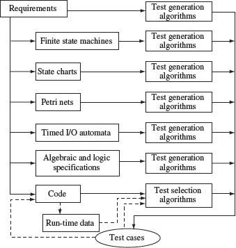
Figure 1.12 Requirements, models, and test generation algorithms.

Another set of strategies falls under the category model based test generation. These strategies require that a subset of the requirements be modeled using a formal notation. Such a model is also known as a specification of a subset of requirements. The tests are then generated with the specification serving as the source. Finite state machines, statecharts, Petri nets, and timed input–output automata are some of the well known and used formal notations for modeling various subsets of requirements. The notations fall under the category graphical notations though textual equivalents also exist. Several other notations, such as sequence and activity diagrams in UML, also exist and are used as models of subsets of requirements.

Languages based on predicate logic as well as algebraic languages are also used to express subsets of requirements in a formal manner. Each of these notational tools have their strengths and weaknesses. Usually, for any large application, one often uses more than notation to express all requirements and generate tests. Algorithms for test generation using finite state models are described in Chapter 5.

There also exist techniques to generate tests directly from the code. Such techniques, fall under code-based test generation. These techniques are useful when enhancing existing tests based on test adequacy criteria. For example, suppose that program Ρ has been tested against tests generated from a statechart specification. After the successful execution of all tests one finds that some of the branches in Ρ have not been covered, that is, there are some conditions that have never evaluated to both true and false. One could now use code-based test generation techniques to generate tests, or modify existing ones, to generate new tests that force a condition to evaluate to true or false, assuming that the evaluations are feasible.

 

Code-based test generation techniques are also used during regression testing when there is often a need to reduce the size of the test suite, or prioritize tests, against which a regression test is to be performed. Such techniques take four inputs, the program to be regression tested P′, the program Ρ from which P′ has been derived by making changes, an existing test suite Τ for P, and some run time information obtained by executing Ρ against T. This run time information may include items such as statement and branch coverage. The test generation algorithm then uses this information to select tests from Τ that must be executed to test those parts of P′ that have changed or are affected by the changes made to P. The resulting test suite is usually a subset of Τ. Techniques for the reduction in the size of a test suite for the purpose of regression testing are described in Chapter 9.

1.11  Static Testing

Static testing is carried out without executing the application under test. This is in contrast to dynamic testing that requires one or more executions of the application under test. Static testing is useful in that it may lead to the discovery of faults in the application, as well as ambiguities and errors in requirements and other application relation documents, at a relatively low cost. This is especially so when dynamic testing is expensive. Nevertheless, static testing is complementary to dynamic testing. Organizations often sacrifice static testing in favor of dynamic testing though this is not considered a good practice.

 

Static testing is best carried out by an individual who did not write the code, or by a team of individuals. A sample process of static testing is illustrated in Figure 1.13. The test team responsible for static testing has access to requirements documents, application, and all associated documents such as design document and user manuals. The team also has access to one or more static testing tools. A static testing tool takes the application code as input and generates a variety of data useful in the test process.

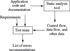
Figure 1.13 Elements of static testing.

1.11.1  Walkthroughs

Walkthroughs and inspections are an integral part of static testing. Walkthrough is an informal process to review any application-related document. For example, requirements are reviewed using a process termed requirements walkthrough. Code is reviewed using code walkthrough, also known as peer code review.

 

A walkthrough begins with a review plan agreed upon by all members of the team. Each item of the document, for example, a source code module, is reviewed with clearly stated objectives in view. A detailed report is generated that lists items of concern regarding the document reviewed.

In requirements walkthrough, the test team must review the requirements document to ensure that the requirements match user needs, and are free from ambiguities and inconsistencies. Review of requirements also improves the understanding of the test team regarding what is desired of the application. Both functional and nonfunctional requirements are reviewed. A detailed report is generated that lists items of concern regarding the requirements.

1.11.2  Inspections

Inspection is a more formally defined process than a walkthrough. This term is usually associated with code. Several organizations consider formal code inspections as a tool to improve code quality at a lower cost than incurred when dynamic testing is used. Organizations have reported significant increases in productivity and software quality due to the use of code inspections.

 

Code inspection is carried out by a team. The team works according to an inspection plan that consists of the following elements: (a) statement of purpose, (b) work product to be inspected, this includes code and associated documents needed for inspection, (c) team formation, roles, and tasks to be performed, (d) rate at which the inspection task is to be completed, and (e) data collection forms where the team will record its findings such as defects discovered, coding standard violations, and time spent in each task.

Members of the inspection team are assigned roles of moderator, reader, recorder, and author. The moderator is in charge of the process and leads the review. Actual code is read by the reader, perhaps with the help of a code browser and with monitors for all in the team to view the code. The recorder records any errors discovered or issues to be looked into. The author is the actual developer whose primary task is to help others to understand the code. It is important that the inspection process be friendly and nonconfrontational. Several books and articles, cited in the Bibliography section, describe various elements of the code inspection process in detail.

1.11.3  Software complexity and static testing

Often a team must decide which of the several modules should be inspected first. Several parameters enter this decision-making process—one of these being module complexity. A more complex module is likely to have more errors and must be accorded higher priority for inspection than a module with lower complexity.

Static analysis tools often compute complexity metrics using one or more complexity metrics discussed in Section 1.6. Such metrics could be used as a parameter in deciding which modules to inspect first. Certainly, the criticality of the function a module serves in an application could override the complexity metric while prioritizing modules.

1.12  Model-Based Testing and Model Checking

Model-based testing refers to the acts of modeling and the generation of tests from a formal model of application behavior. Model checking refers to a class of techniques that allow the validation of one or more properties from a given model of an application.

 

Figure 1.14 illustrates the process of model checking. A model, usually in finite state, is extracted from some source. The source could be the requirements and, in some cases, the application code itself. Each state of the finite state model is prefixed with one or more properties that must hold when the application is in that state. For example, a property could be as simple as “x < 0” indicating that variable x must hold a negative value in this state. More complex properties, such as those related to timing, may also be associated.

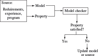
Figure 1.14 Elements of model checking.

One or more desired properties are then coded in a formal specification language. Often, such properties are coded in temporal logic, a language for formally specifying timing properties. The model and the desired properties are then input to a model checker. The model checker attempts to verify whether or not the given properties are satisfied by the given model.

For each property, the checker could come up with one of three possible answers: the property is satisfied, the property is not satisfied, or unable to determine. In the second case, the model checker provides a counterexample showing why the property is not satisfied. The third case might arise when the model checker is unable to terminate after an upper limit on the number of iterations has reached.

In almost all cases, a model is a simplified version of the actual system requirements. A positive verdict by the model checker does not necessarily imply that the stated property is indeed satisfied in all cases. Hence, the need for testing. Despite a positive verdict by the model checker, testing is necessary to ascertain at least for a given set of situations that the application indeed satisfies the property.

While both model checking and model-based testing use models, model checking uses finite state models augmented with local properties that must hold at individual states. The local properties are known as atomic propositions and the augmented models as Kripke structures.

In summary, model checking is to be viewed as a powerful and complementary technique to model-based testing. Neither can guarantee whether an application satisfies a property under all input conditions. However, both point to useful information that helps a tester to discover sometimes subtle errors.

1.13  Types of Testing

An answer to the question “What types of testing are performed in your organization ?” often consists of a set of terms such as black-box testing, reliability testing, unit testing, and so on. There exist a number of terms that typify one or more types of testing. We abstract all these terms as “X-testing.” In this section, we present a framework for the classification of testing techniques. We then use this framework to classify a variety of testing techniques by giving meaning to the “X” in “X-testing.”

Our framework consists of a set of four classifiers that serve to classify testing techniques that fall under the “dynamic testing” category. Techniques that fall under the “static testing”category are discussed in Section 1.11. Dynamic testing requires the execution of the program under test. Static testing consists of techniques for the review and analysis of the program.

Each of the four classifiers is a mapping from a set of features to a set of testing techniques. Features include source of test generation, questions that define a goal, a phase of life cycle or an artifact. Here are the four classifiers labeled as C1 through C4.

1. C1: Source of test generation
2. C2: Life cycle phase in which testing takes place
3. C3: Goal of a specific testing activity
4. C4: Characteristics of the artifact under test
5. C5: Test process

Tables 1.4 through 1.8 list each classifier by specifying the mapping and provide a few examples where appropriate. While each classifier defines a mapping, there exists a hierarchy across mappings. For example, black-box testing is used in almost all goal-directed testing. As is evident from the table, each mapping is not necessarily one-to-one. For example, pairwise testing could be used to design tests for an entire system or for a component.

 

Table 1.4 Classification of techniques for testing computer software. Classifier: C1: Source of test generation.

Artifact	Technique	Example
Requirements(informal)	Black-box	Ad-hoc testing Boundary value analysis Category partition Classification trees Cause–effect graphs Equivalence partitioning Partition testing Predicate testing Random testing Syntax testing
Code	White-box	Adequacy assessment Coverage testing Data-flow testing Domain testing Mutation testing Path testing Structural testing Test minimization
Requirements and code	Black-box and White-box
Formal model: Graphical or mathematical specification	Model-based Specification	Statechart testing FSM testing Pairwise testing Syntax testing
Component interface	Interface testing	Interface mutation Pairwise testing

Test techniques that fall under mapping C1 are more generic than others. Each technique under C1 is potentially applicable to meet the goal specified in C3 as well as to test the software objects in C4. For example, one could use pairwise testing as a means to generate tests in any goal-directed testing that falls within C3. Let us now examine each classifier in more detail.

1.13.1  Classifier: C1: Source of test generation

Black-box testing: Test generation is an essential part of testing; it is as wedded to testing as the Earth is to the Sun. There are a variety of ways to generate tests; some are listed in Table 1.4. Tests could be generated from informally or formally specified requirements and without the aid of the code that is under test. Such form of testing is commonly referred to as black-box testing. When the requirements are informally specified, one could use ad-hoc techniques or heuristics such as equivalence partitioning and boundary value analysis.

 

Model-based or specification-based testing: Model-based or specification-based testing occurs when the requirements are formally specified, as for example, using one or more mathematical or graphical notations such as Z, state charts, and an event sequence graph, and tests are generated using the formal specification. This is also a form of black box testing. As listed in Table 1.4, there are a variety of techniques for generating tests for black-box and model-based testing. Part II of this book introduces several of these.

White-box testing: White-box testing refers to the test activity wherein code is used in the generation of, or the assessment of, test cases. It is rare, and almost impossible, to use white-box testing in isolation. As a test case consists of both inputs and expected outputs, one must use requirements to generate test cases; the code is used as an additional artifact in the generation process. However, there are techniques for generating tests exclusively from code and the corresponding expected output from requirements. For example, tools are available to generate tests to distinguish all mutants of a program under test or generate tests that force the program under test to exercise a given path. In any case, when someone claims they are using white-box testing, it is reasonable to conclude that they are using some forms of both black-box and white-box testing.

 

Code could be used directly or indirectly for test generation. In the direct case, a tool, or a human tester, examines the code and focuses on a given path to be covered. A test is generated to cover this path. In the indirect case, tests generated using some black-box technique are assessed against some code-based coverage criterion. Additional tests are then generated to cover the uncovered portions of the code by analyzing which parts of the code are feasible. Control flow, data flow, and mutating testing can be used for direct as well as indirect code-based test generation.

Interface testing: Tests are often generated using a component’s interface. Certainly, the interface itself forms a part of the component’s requirements and hence this form of testing is black-box testing. However, the focus on interface leads us to consider interface testing in its own right. Techniques such as pairwise testing and interface mutation are used to generate tests from a component’s interface specification. In pairwise testing, the set of values for each input is obtained from the component’s requirement. In interface mutation, the interface itself, such as a function coded in C or a CORBA component written in an IDL, serves to extract the information needed to perform interface mutation. While pairwise testing is clearly a black-box testing technique, interface mutation is a white-box technique though it focuses on the interface-related elements of the component under test.

 

Ad-hoc testing is not to be confused with random testing. In ad-hoc testing, a tester generates tests from requirements but without the use of any systematic method. Random testing uses a systematic method to generate tests. Generation of tests using random testing requires modeling the input space and then sampling data from the input space randomly.

In summary, black-box and white-box are the two most fundamental test techniques; they form the foundation of software testing. Test generation and assessment techniques are at the foundation of software testing. All the remaining test techniques classified by C2 through C4 fall into either the black-box or the white-box category.

1.13.2  Classifier: C2: Life cycle phase

Testing activities take place throughout the software life cycle. Each artifact produced is often subject to testing at different levels of rigor and using different testing techniques. Testing is often categorized based on the phase in which it occurs. Table 1.5 lists various types of testing depending on the phase in which the activity occurs.

 

Table 1.5 Classification of techniques for testing computer software. Classifier: C2: Life cycle phase.

Phase	Technique
Coding	Unit testing
Integration	Integration testing
System integration	System testing
Maintenance	Regression testing
Post system, pre-release	Beta-testing

Programmers write code during the early coding phase. They test their code before it is integrated with other system components. This type of testing is referred to as unit testing. When units are integrated and a large component or a subsystem formed, one does integration testing of the subsystem. Eventually, when the entire system has been built, its testing is referred to as system testing.

Test phases mentioned above differ in their timing and focus. In unit testing, a programmer focuses on the unit or a small component that has been developed. The goal is to ensure that the unit functions correctly in isolation. In integration testing, the goal is to ensure that a collection of components function as desired. Integration errors are often discovered at this stage. The goal of system testing is to ensure that all the desired functionality is in the system and works as per its requirements. Note that tests designed during unit testing are not likely to be used during integration and system testing. Similarly, tests designed for integration testing might not be useful for system testing.

 

Often a carefully selected set of customers are asked to test a system before release. This form of testing is referred to as beta-testing. In the case of contract software, the customer who contracted the development performs acceptability testing prior to making the final decision as to whether or not to purchase the application for deployment.

Errors reported by users of an application often lead to additional testing and debugging. Often times, changes made to an application are much smaller in their size when compared to the entire application thus obviating the need for a complete system test. In such situations, one performs a regression test. The goal of regression testing is to ensure that the modified system functions per its specifications. However, regression testing may be performed using a subset of the entire set of test cases used for system testing. Test cases selected for regression testing include those designed to test the modified code and any other code that might be affected by the modifications.

It is important to note that all black-box and white-box testing techniques mentioned in Table 1.4 are applicable during each life cycle phase when code is being tested. For example, one could use the pairwise testing technique to generate tests for integration testing. One could also use any white box technique, such as test assessment and enhancement, during regression testing.

1.13.3  Classifier: C3: Goal-directed testing

Goal-directed testing leads to a large number of terms in software testing. Table 1.6 lists a sample of goals commonly used in practice, and the names of the corresponding test techniques.

 

Table 1.6 Classification of techniques for testing computer software. Classifier: C3: Goal-directed testing.

Goal	Testing Technique	Example
Advertised features	Functional
Security	Security
Invalid inputs	Robustness
Vulnerabilities	Vulnerability	Penetration testing
Errors in GUI	GUI	Capture/playback Event sequence graphs Complete Interaction Sequence
Operational correctness	Operational	Transactional-flow
Reliability assessment	Reliability
Resistance to penetration	Penetration
System performance	Performance	Stress testing
Customer acceptability	Acceptance
Business compatibility	Compatibility	Interface testing Installation testing
Peripherals compatibility	Configuration
Foreign language compatibility	Foreign language

 

There exists a variety of goals. Of course, finding any hidden errors is the prime goal of testing; goal-oriented testing looks for specific types of failures. For example, the goal of vulnerability testing is to detect if there is any way by which the system under test can be penetrated by unauthorized users. Suppose that an organization has set up security policies and taken security measures. Penetration testing aims at evaluating how good these policies and measures are. Again, both black-box and white box techniques for the generation and evaluation of tests are applicable to penetration testing. Nevertheless, in many organizations, penetration and other forms of security testing remain ad-hoc.

Robustness testing: Robustness testing refers to the task of testing an application for robustness against unintended inputs. It differs from functional testing in that the tests for robustness are derived from outside of the valid (or expected) input space whereas in the former the tests are derived from the valid input space.

 

As an example of robustness testing, suppose that an application is required to perform a function for all values of x ≥ 0. However, there is no specification of what the application must do for x < 0. In this case, robustness testing would require that the application be tested against tests where x < 0. As the requirements do not specify behavior outside the valid input space, a clear understanding of what robustness means is needed for each application. In some applications, robustness might simply mean that the application displays an error message and exits, while in others, it might mean that the application brings an aircraft to a safe landing!

Stress testing: In stress testing, one checks for the behavior of an application under stress. Handling of overflow of data storage, for example, buffers, can be checked with the help of stress testing. Web applications can be tested by “stressing” them with a large number and variety of requests. The goal here is to find if the application continues to function correctly under stress.

 

One needs to quantify “stress” in the context of each application. For example, a web service can be stressed by sending it an unusually large number of requests. The goal of such testing would be to check if the application continues to function correctly and performs its services at the desired rate. Stress testing checks an application for conformance to its functional requirements as well as to its performance requirements when under stress.

Performance testing: The term “performance testing” refers to that phase of testing where an application is tested specifically with performance requirements in view. For example, a compiler might be tested to check if it meets the performance requirements stated in terms of the number of lines of code compiled per second.

 

Often performance requirements are stated with respect to a hardware and software configuration. For example, an application might be required to process 1000 billing transactions per minute on a specific Intel processor based machine and running a specific operating system.

Load testing: The term “load testing” refers to that phase of testing in which an application is “loaded” with respect to one or more operations. The goal is to determine if the application continues to perform as required under various load conditions. For example, a database server can be loaded with requests from a large number of simulated users. While the server might work correctly when one or two users use it, it might fail in various ways when the number of users exceeds a threshold.

During load testing, one can determine whether or not the application is handling exceptions in an adequate manner. For example, an application might maintain a dynamically allocated buffer to store user IDs. The buffer size increases with an increase in the number of simultaneous users. There might be a situation when additional memory space is not available to add to the buffer. A poorly designed, or incorrectly coded, application might crash in such a situation. However, a carefully designed and correctly coded application will handle the “out of memory” exception in a graceful manner such as by announcing the high load through an apology message.

In a sense, load testing is yet another term for stress testing. However, load testing can be performed for ascertaining an application’s performance as well as the correctness of its behavior. It is a form of stress testing when the objective is to check for correctness with respect to the functional requirements under load. It is a form of performance testing when the objective is to assess the time it takes to perform certain operations under a range of given conditions.

Load testing is also a form of robustness testing, i.e., testing for unspecified requirements. For example, there might not be any explicitly stated requirement related to the maximum number of users an application can handle and what the application must do when the number of users exceeds a threshold. In such situations, load testing allows a tester to determine the threshold beyond which the application under test fails through, e.g. a crash.

Terminology overlap: Note that there is some overlap in the terminology. For example, vulnerability testing is a form of security testing. Also, testing for compatibility with business goals might also include vulnerability testing. Such overlaps abound in testing-related terminology.

Once again note that formal techniques for test generation and test adequacy assessment apply to all forms of goal-directed testing. A lack of examples in almost the entire Table 1.6 is because test generation and assessment techniques listed in Table 1.4 are applicable to goal-directed testing. It is technically correct to confess “We do ad-hoc testing” when none of the formal test generation techniques are used.

1.13.4  Classifier: C4: Artifact under test

Testers often say “We do X-testing” where X corresponds to an artifact under test. Table 1.7 is a partial list of testing techniques named after the artifact that is being tested. For example, during the design phase one might generate a design using the SDL notation. This design can be tested before it is committed to code. This form of testing is known as design testing.

 

Table 1.7 Classification of techniques for testing computer software. Classifier: C4: Artifact under test.

Characteristic	Technique
Application component	Component testing
Batch processing	Equivalence partitioning, finite state model based testing, and most other test generation techniques discussed in this book
Client and server	Client-server testing
Compiler	Compiler testing
Design	Design testing
Code	Code testing
Database system	Transaction-flow testing
OO software	OO testing
Operating system	Operating system testing
Real-time software	Real-time testing
Requirements	Requirements testing
Web service	Web service testing

As another example, you might have seen articles and books on OO-testing. Again, OO-testing refers to the testing of programs that are written in an object-oriented language such as C++ or Java. Yet again, there exists a variety of test generation and adequacy assessment techniques that fall under black-box and white-box categories and that are applicable to the testing of OO software.

It is important to note that specialized black-box and white-box test techniques are available for specialized software. For example, timed-automata and Petri net-based test generation techniques are intended for the generation of tests for real-time software.

Batch processing applications pose a special challenge in testing. Payroll processing in organization and student record processing in academic institutions are two examples of batch processing. Often, these applications perform the same set of tasks on a large number records, for example, an employee record or a student record. Using the notions of equivalence partitioning and other requirements based test generation techniques discussed in Chapter 3, one must first ensure that each record is processed correctly. In addition, one must test for performance under heavy load, which can be done using load testing. While testing a batch processing application, it is also important to include an oracle that will check the result of executing each test script. This oracle might be a part of the test script itself. It could, for example, query the contents of a database after performing an operation that is intended to change the status of the database.

Sometimes an application might not be a batch processing application though a number of tests may need to be run in a batch. An embedded application, such as a cardiac pacemaker, is where there is a need to develop a set of tests that need to be run in a batch. Often, organizations develop a specialized tool to run a set of tests as a batch. For example, the tests might be encoded as scripts. The tool takes each test script and applies the test to the application. In a situation like this, the tool must have facilities such as to interrupt a test, suspend a test, resume a test, check test status, and schedule the batch test. IBM’s WebSphere Studio is one of the several tools available for the development and testing of batch processing applications built using the J2EE environment.

1.13.5  Classifier: C5: Test process models

Software testing can be integrated into the software development life cycle in a variety of ways. This leads to various models for the test process listed in Table 1.8. Some of the models are described next.

 

Table 1.8 Classification of techniques for testing computer software. Classifier: C5: Test process models.

Process	Attributes
Testing in waterfall model	Usually done toward the end of the development cycle.
Testing in V model	Explicitly specifies testing activities in each phase of the development cycle.
Spiral testing	Applied to software increments, each increment might be a prototype that eventually leads to the application delivered to the customer. Proposed for evolutionary software development.
Agile testing	Used in agile development methodologies such as extreme programming (XP).
Test Driven Development (TDD)	Requirements specified as tests.

Testing in the waterfall model: The waterfall model is one of the earliest, and least used, software life cycle models. Figure 1.15 shows the different phases in a development process based on the waterfall model. While verification and validation of documents produced in each phase is an essential activity, static as well as dynamic testing occurs toward the end of the process. Further, as the waterfall model requires adherence to an inherently sequential process, defects introduced in the early phases and discovered in later phases could be costly to correct. There is very little iterative or incremental development when using the waterfall model.

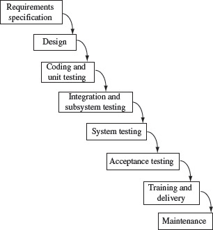
Figure 1.15 Testing in the waterfall model. Arrows indicate the “flow” of documents from one to the next. For example, design documents are input to the coding phase. The waterfall nature of the flow led to the name of this model.

Testing in the V model: The V-model, as shown in Figure 1.16, explicitly specifies testing activities associated with each phase of the development cycle. These activities begin from the start and continue until the end of the life cycle. The testing activities are carried out in parallel with the development activities. Note that the V-model consists of the same development phases as in the waterfall model; the visual layout and an explicit specification of the test activities are the key differentiators. It is also important to note that test design begins soon after the requirements are available.

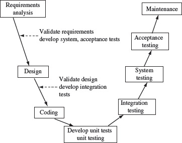
Figure 1.16 Testing in the V model.

Spiral testing: The term “spiral testing” is not to be confused with spiral model, though they are both similar as both can be visually represented as a spiral of activities as in Figure 1.17. The spiral model is a generic model that can be used to derive process models such as the waterfall model, the V-model, and the incremental development model. While testing is a key activity in the spiral model, spiral testing refers to a test strategy that can be applied to any incremental software development process especially where a prototype evolves into an application. In spiral testing the sophistication of test activities increases with the stages of an evolving prototype.

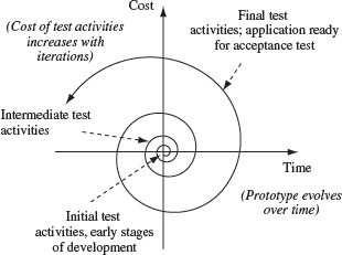
Figure 1.17 A visual representation of spiral testing. Test activities evolve over time and with the prototype. In the final iteration, the application is available for system and acceptance testing.

In the early stages, when a prototype is used to evaluate how an application must evolve, one focuses on test planning. The focus at this stage is on how testing will be performed in the remainder of the project. Subsequent iterations refine the prototype based on a more precise set of requirements. Further test planning takes place and unit and integration tests are performed. In the final stage, when the requirements are well defined, testers focus on system and acceptance testing. Note that all test generation techniques described in this book are applicable in the spiral testing paradigm. Note from Figure 1.17 that the cost of the testing activities (vertical axis) increases with subsequent iterations.

Agile testing: This is a name given to a test process that is rarely well defined. One way to define it is to specify what agile testing involves in addition to the usual steps such as test planning, test design, and test execution. Agile testing promotes the following ideas: (a) include testing related activities throughout a development project starting from the requirements phase, (b) work collaboratively with the customer who specifies requirements in terms of tests, (c) testers and developers must collaborate with each other rather than serve as adversaries, and (d) test often and in small chunks.

While there exist a variety of models for the test process, the test generation and adequacy techniques described in this are applicable to all. Certainly, focus on test process is an important aspect of the management of any software development process.

The next example illustrates how some of the different types of testing techniques can be applied to test the same piece of software. The techniques so used can be easily classified using one or more of the classifiers described above. 

Example 1.21   Consider a web service W to be tested. When executed, W converts a given value of temperature from one scale to another, for example from the Fahrenheit scale to the Celsius scale. Regardless of the technique used for test generation, we can refer to the testing of W as web-services testing. This reference uses the C4 classifier to describe the type of testing.

Next, let us examine various types of test generation techniques that could be used for testing W. First, suppose that tester A tests W by supplying sample inputs and checking the outputs. No specific method is used to generate the inputs. Using classifier C1, one may say that A has performed black-box testing and used an ad-hoc, or exploratory, method for test data generation. Using classifier C2 one may say that A has performed unit testing on W, assuming that W is a unit of a larger application. Given that W has a GUI to interface with a user, one can use classifier C3 and say that A has performed GUI testing.

Now suppose that another tester Β writes a set of formal specifications for W using the Ζ notation. The tester generates, and uses, tests from the specification using techniques described in Volume 2. In this case, again using classifier C1, one may say that tester Β has performed black-box testing and used a set of specification-based algorithms for test data generation.

Let us assume that we have a smarter tester C who generates tests using the formal specifications for W. C then tests W and evaluates the code coverage using one of the several code coverage criteria. C finds that the code coverage is not 100%, that is, some parts of the code inside W have remained uncovered, that is, untested, by the tests generated using the formal specification. C then generates and runs additional tests with the objective of exercising the uncovered portions of W. We say that here, C has performed both black-box and white-box testing. C has used specification-based test generation and enhanced the tests so generated to satisfy some control-flow based code coverage criteria.

Now, suppose that tester D tests W as a component of a larger application. Tester D does not have access to the code for W and hence uses only its interface, and interface mutation, to generate tests. Using classifier C1 one may say that tester D has performed black-box testing and used interface mutation to generate tests (also see Exercise 1.17).

It should be obvious from the above example that simply using one classifier to describe a test technique might not provide sufficient information regarding details of the testing performed. To describe the set of testing techniques used to test any software object, one must clearly describe the following:

1. Test generation methods used; number of tests generated; number of tests run; number of tests failed and number passed.
2. Test adequacy assessment criteria used; results of test assessment stated in quantitative terms.
3. Test enhancement: number of additional tests generated based on the outcome adequacy assessment; number of additional tests run; number of additional failures discovered.

Note that test generation, adequacy assessment, and enhancement must be treated as a set of integrated activities. It is the sophistication of these activities, and their execution, that constitutes one important determinant of the quality of the delivered product.

1.14  The Saturation Effect

The saturation effect is an abstraction of a phenomenon observed during the testing of complex software systems. Refer to Figure 1.18 to understand this important effect. The horizontal axis in the figure indicates the test effort that increases over time. The test effort can be measured as, for example, the number of test cases executed or total person days spent during the test and debug phase. The vertical axis refers to the true reliability (solid lines) and the confidence in the correct behavior (dotted lines) of the application under test. Note that the application under test evolves with an increase in test effort due to error correction.

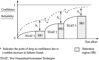
Figure 1.18 The saturation effect observed during the testing of complex software systems.

The vertical axis can also be labeled as the “cumulative count of failures” that are observed over time, that is, as the test effort increases. The error correction process usually removes the cause of one or more failures. However, as the test effort increases additional failures may be found that causes the cumulative failure count to increase though it saturates as shown in the figure.

1.14.1  Confidence and true reliability

“Confidence” in Figure 1.18 refers to the confidence of the test manager in the true reliability of the application under test. An estimate of reliability, obtained using a suitable statistical method, can be used as a measure of confidence. “Reliability” in the figure refers to the probability of failure-free operation of the application under test in its intended environment. The “true” reliability differs from the estimated reliability in that the latter is an estimate of the application reliability obtained by using one of the many statistical methods. A 0 indicates lowest possible confidence and 1 the highest possible confidence. Similarly, a 0 indicates the lowest possible true reliability and a 1 indicates the highest possible true reliability.

1.14.2  Saturation region

Now suppose that application A is in the system test phase. The test team needs to generate tests, encapsulate them into appropriate scripts, set up the test environment, and run A against the tests. Let us assume that the tests are generated using a suitable test generation method (referred to as TGAT1 in Figure 1.18) and that each test either passes or fails. Each failure is analyzed and fixed, perhaps by the development team, if it is determined that A must not be shipped to the customer without fixing the cause of this failure. Whether the failure is fixed soon or later after it is detected, does not concern us in this discussion.

The true reliability of A, with respect to the operational profile used in testing, increases as errors are removed. Certainly, the true reliability could decrease in cases where fixing an error introduces additional errors–a case that we ignore in this discussion. If we measure the test effort as the combined effort of testing, debugging, and fixing the errors, the true reliability increases as shown in Figure 1.18 and eventually saturates, that is, stops increasing. Thus, regardless of the number of tests generated, and given the set of tests generated using TGAT1, the true reliability stops increasing after a certain amount of test effort has been spent. This saturation in the true reliability is shown in Figure 1.18 as the shaded region labeled SR1. Inside SR1, the true reliability remains constant while the test effort increases.

No new faults are found and fixed in the saturation region. Thus, the saturation region is indicative of wasted test effort under the assumption that A contains faults not detected while the test phase is in the saturation region.

1.14.3  False sense of confidence

The discovery and fixing of previously undiscovered faults might increase our confidence in the reliability of A. It also increases the true reliability of A. However, in the saturation region when the expenditure of test effort does not reveal new faults, the true reliability of A remains unchanged though our confidence is likely to increase due to a lack of observed failures. While in some cases this increase in confidence might be justified, in others it is a false sense of confidence.

This false sense of confidence is due to the lack of discovery of new faults, which in turn is due to the inability of the tests generated using TGAT1 to exercise the application code in ways significantly different from what has already been exercised. Thus, in the saturation region, the robust states of the application are being exercised, perhaps repeatedly, whereas the faults lie in other states.

The symbol Δ₁ in Figure 1.18 is a measure of the deviation from the true reliability of A and a test manager’s confidence in the correctness of A. While one might suggest that Δ₁ can be estimated given an estimate of the confidence and the true reliability, in practice it is difficult to arrive at such an estimate due to the fuzzy nature of the confidence term. Hence, we must seek a quantitative metric that replaces human confidence.

1.14.4  Reducing Δ

Empirical studies reveal that every single test generation method has its limitations in that the resulting test set is unlikely to detect all faults in an application. The more complex an application, the more unlikely it is that tests generated using any given method will detect all faults. This is one of the prime reasons why testers use, or must use, multiple techniques for test generation.

Suppose that a black-box test generation method is used to generate tests. For example, one might express the expected behavior of A using a finite state model and generate tests from the model as described in Chapter 5. Let us denote this method as TGAT1 and the test set so generated as T1.

Now, suppose that after having completed the test process using T1, we check how much of the code in A has been exercised. There are several ways to perform this check, and suppose that we use a control flow-based criterion, such as the MC/DC criterion described in Chapter 7. It is likely that T1 is inadequate with respect to the MC/DC criterion. Hence, we enhance T1 to generate T2, which is adequate with respect to the MC/DC criterion and T1 ⊂ T2. We refer to this second method of test generation as TGAT2.

Enhancement of tests based on feedback received from adequacy assessment leads to tests that are likely to move A to at least a few states that were never covered when testing using T1. This raises the possibility of detecting faults that might lie in the newly covered states. In the event, a failure occurs as a consequence of executing A against one or more tests in T2, the confidence exhibits a dip while the true reliability increases, assuming that the fault that caused the failure is removed and none introduced. Nevertheless, the true reliability once again reaches the saturation region, this time SR2.

The process described above for test enhancement can now be repeated using a different and perhaps a more powerful test adequacy criterion. The new test generation and enhancement technique is referred to in Figure 1.18 as TGAT3. The test set generated due to enhancement is T3 and T2 ⊂ T3. Once again we observe a dip in confidence, an increase in the true reliability, and eventually entry into the saturation region–SR3 in this case. Note that it is not always necessary that enhancement of a test set using an adequacy criteria will lead to a larger test set. It is certainly possible that T1=T2 or that T2=T3. However, this is unlikely to happen in a large application.

Theoretically the test generation and enhancement procedure described above can proceed almost forever especially when the input domain is astronomical in size. In practice, however, the process must terminate so that the application can be released. Regardless of when the application is released, it is likely that Δ > 0 implying that while the confidence may be close to the true reliability, it is unlikely to be equal.

1.14.5  Impact on test process

A knowledge and appreciation of the saturation effect will likely be of value to any test team while designing and implementing a test process. Given that any method for the construction of functional tests will likely lead to a test set that is inadequate with respect to the code-based coverage criteria, it is important that tests be assessed for their goodness.

Various goodness measures are discussed in Chapters 7 and 8. It is some code coverage criterion that leads to saturation shown in Figure 1.18. For example, execution of additional tests might not lead to the coverage of any uncovered conditions. Enhancing tests using one or more code-based coverage criteria will likely help in moving out of a saturation region.

As the assessment of the goodness of tests does not scale well with the size of the application, it is important that this be done incrementally and using the application architecture. This aspect of test assessment is also covered in Chapters 7 and 8.

1.15  Principles of Testing

A principle, according to a definition, is a law that is usually followed. Principles can exist in several forms. A principle could be as a cause. For example, there exists principle of causality, or as a scientific law, a moral law, etc. Principles of software testing can be derived from experience, mathematical facts, and empirical studies. This section enumerates a few principles of software testing. In 2009, Bertrand Meyers postulated seven principles of software testing. The principles listed below are different from those proposed by Meyers, though one may find some similarity.

Principle 1: Definition

Testing is the activity of assessing how well a program behaves in relation to its expected behavior.

Complex software, such as an OS or a database system, can rarely be proven correct. Testing is the means to gain confidence in the correctness of the software. The level of confidence so gained depends on the individual viewing the test results as well as the number of successes and failures.

Principle 2: Reliability and confidence

Testing may increase one’s confidence in the correctness of a program though the confidence may not match with the program’s reliability.

A program’s reliability is a statistical measure of its probability of successful operation in a given environment. It is estimated on a random test derived from an operational profile. Unless the operational profile is a close estimation of the expected usage scenario, a rare practical occurrence, the estimated reliability would likely be higher than the “true” reliability. Thus, while a diminishing rate of failures during testing increases reliability estimates, it may not necessarily increase the “true” reliability.

Principle 3: Coverage

A test case that tests untested portions of a program enhances or diminishes one’s confidence in the program’s correctness depending on whether the test passes or fails.

Principle 4: Orthogonality

Statistical measurements of the reliability of an application and the code coverage obtained by the tests used for measuring the reliability are orthogonal.

When an untested portion of the program passes a test, it increases one’s confidence in the program correctness while a failure decreases the confidence. This implies that a good test suite consists of tests that test different portions of the code further implying that each test improves code coverage in some way.

Principle 5: Test suite quality

Code coverage is a reliable metric for the quality of a test suite.

Indeed, obtaining 100% code coverage does not imply correctness. However, tests that pass and improve code coverage lead to increased confidence in program correctness. A test suite adequate with respect to a coverage metric is likely to be better in terms of its error-revealing capability than another adequate with respect to a less powerful coverage metric.

Principle 6: Requirements and tests

Tests derived manually from requirements alone are rarely complete.

Complex systems are likely to have complex requirements. A complex set of requirements is difficult to understand in its entirety by any single individual. Thus, while a team of testers might generate tests to cover each requirement at least once, generating tests to cover the complex interactions across the individual requirements becomes an almost impossible task. This observation makes it important for test organizations to create one or more objective measures of test completeness.

Principle 7: Random testing

Random testing may or may not outperform nonrandom testing.

Random testing is a useful strategy to assess the robustness of a program. There is no guarantee that randomly generated tests will work better than a much smaller suite of tests generated using formal methods and aimed at functional testing. However, in many cases, random testing can outperform nonrandom testing especially when the aim is to check for any undesirable extreme behavior of a program such as a crash or a hang.

Principle 8: Saturation effect

The saturation effect is real and can be used as an effective tool for the improvement of test generation strategies.

Regardless of the test generation technique used, the rate at which latent faults are discovered is likely to be zero after a certain number of tests have been executed. To improve the “true” reliability of the program, it is best to switch to a different strategy for test generation.

Principle 9: Automation

Test automation aids in reducing the cost of testing and making it more reliable, but not necessarily in all situations.

Running a large number of tests manually and checking the outcome is indeed costly and error prone. Thus, test automation ought to be considered seriously in any system test environment. However, the cost of automating the test process needs to be weighed carefully against the benefits. While there exist several tools that automate the process of test generation, they do not overcome the problem of automating the process of generating an oracle that determines whether an automatically generated test passes or not.

Principle 10: Metrics

Integrating metrics into the entire test process aids in process improvement.

An organization-wide metrics program ought to include metrics related to all aspects of the test process. Such metrics, collected with help from tools, is helpful in assessing the improvement of, or otherwise, the quality of the test process and the released products.

Principle 11: Roles

Every developer is also a tester.

A developer is expected to write correct code, that is code that meets the requirements. While a developer could use model checking and other formal methods for proving the correctness of the written code, these are no substitutes for thorough testing. Thus, every developer ought to assume the role of a tester to ensure quality units that are to be integrated into a system.

1.16  Tools

A sample of tools useful for various types of testing that are not covered in any significant detail in this book is enumerated below. These include tools for performance, load, and stress testing, and for test management.

 

Tool: WinRunner (HP Functional Testing)

Link: http://en.wikipedia.org/wiki/HP_Application_Lifecycle_Management#HP_Functional_Testing

Description

 

A well-known load-testing tool named “WinRunner” is now integrated into HP Functional Test suite. This suite consists of several tools for business process testing, functional, load, performance testing as well as for test data management.

 

Tool: JMeter

Link: http://jmeter.apache.org/

Description

 

JMeter is an open source Java application intended for load testing. It can load a variety of servers including HTTP, HTTPS, SOAP, and IMAP. It is multithreaded and hence allows concurrent sampling of various testing functions. JMeter has a GUI through which a test is controlled. JMeter serves as a master controller that controls multiple slave JMeter servers. Each server can send test commands to the target systems under test. Thus, JMeter serves to perform distributed testing.

 

Tool: JavaMetrics

Link: http://www.semdesigns.com/products/metrics/JavaMetrics.html

Description

 

JavaMetrics is sold by Semantic Designs. It calculates a variety of metrics from Java programs. The metrics include Source Lines of Code (SLOC), number of methods, decision density, cyclomatic complexity, and others. The same company makes similar tool for other languages including C#, COBOL, and VBScript.

 

Tool: COCOMO II

Link: http://diana.nps.edu/madachy/tools/COCOMOII.php

Description

 

COCOMO (Constructive Cost Model) II is a tool for estimating software development effort and cost. This is an online tool that asks a user to enter a set of parameters that describe the software under development. These parameters are divided into two categories: scale drivers and cost drivers. Scale drivers include parameters such as development flexibility and process maturity. Cost drivers include parameters such as product complexity, programmer capability, application experience, and multisite development.

 

Tool: Bugzilla

Link: http://www.bugzilla.org/

Description

 

Bugzilla is a freely available application for tracking defects. It allows developers and testers to keep track of defects in their application. It allows communications among team members. The Mozilla Foundation, developer of Firefox, uses Bugzilla regularly.

 

Tool: Testopia

Link: http://www.mozilla.org/projects/testopia/

Description

 

This tool is an extension of the bug reporting and management tool Bugzilla. It allows the integration of test results with bug reports.

 

Tool: IBM Rational ClearCase

Link: http://en.wikipedia.org/wiki/IBM_Rational_ClearCase

Description

 

ClearCase is a family of tools that support test configuration management. It can be used to specify configurations using one of two use models: Unified Change Management (UCM) and base ClearCase.

 

Exercises

1.1 The following statement is often encountered: “It is impossible to test a program completely.” Discuss the context in which this statement is true. Under what definition of “completely” is the statement true ? (Note: Try answering this question now and return to it after having read Chapter 7.)

1.2 Describe at least one case in which a “perceived” incorrect behavior of a product is not due to an error in the product.

1.3 How many years will it take to test max exhaustively on a computer that takes 1 picosecond (= 10^–12 seconds) to input a pair of integers and execute max ?

1.4 It is required to develop a strategy to test whether or not a joke is excellent, good, or poor. What strategy would you propose? Would statistical techniques be useful in categorizing a joke?

1.5 Estimate the reliability of Ρ of Example 1.12 given that (a) the input pair (0, 0) appears with probability 0.6 and the remaining two pairs appear with probability 0.2 each and (b) Ρ fails on the input (– 1, 1).

1.6 According to the ANSI/IEEE Std 729-1983, is it possible for a program to have a reliability of 1.0 even when it is infected with a number of defects ? Explain your answer.

1.7 Suppose that the sort program in Example 1.13 is known to fail with probability 0.9 when alphanumeric strings are input and that it functions correctly on all numeric inputs. Find the reliability of sort with respect to the two operational profiles in Example 1.13.

1.8 Suggest one possible coding of sort that will lead to the behavior given in Example 1.9.

1.9 Consider a Web site that allows its visitors to search for items in a database using arbitrary search strings. Suppose we focus our attention only on three operations allowed by this site: search, previous, and next. To invoke the search operation, a search string is typed and the Go button clicked. When the search results are displayed, the Previous and Next buttons show up and may be clicked to move to the next or the previous page of search results. Describe how an oracle will determine whether or not the three functions of the Web site are implemented correctly. Can this oracle be automated ?

1.10 Suggest a procedure to estimate the efficiency of a test set.

1.11 Let T₁ and T₂ be test sets designed to test how well program Ρ meets requirements R. Suppose that the efficiency of both test sets is the same, (a) What features of the two test sets would you use to decide which one to select?

1.12 (a) Compute the cyclomatic complexity of the CFG in Figure 2.2 of the next chapter. (b) Prove that for CFGs of structured programs, the cyclomatic complexity is the number of conditions plus one. A structured program is one that uses only single entry and single exit constructs. GOTO statements are not allowed in a structured program.

1.13 For the two programs P1.1 and P1.2 compute Halstead’s software science metrics. Discuss the relative complexity of the two programs using the metrics you have computed. Note the following while computing the software science metrics: (i) each token in a program, excluding semicolon (;) and braces, is to be considered as either an operator or an operand, (ii) each declaration keyword is an operator and the variable declared an operand, Thus, for example, keywords such as if and else, and function calls, are operators and so are the traditional arithmetic and relational symbols such as < and +.

1.14 Consider two applications A₁ and A₂. Suppose that the testability of these applications is measured using a static complexity measure such as the cyclomatic complexity. Now suppose that the cyclomatic complexity of both applications is the same. Construct an example to show that despite the same cyclomatic complexity the testability of A₁ and A₂ might differ significantly. (Hint: Think of embedded applications.)

1.15 Consider a 2-input NAND gate in Figure 1.11 (a) with the following faults: (i) input A stuck at 0 and output Ο stuck at 1, (ii) input A stuck at 0 and output Ο stuck at 0, (iii) inputs A and Β stuck at 1, (iv) inputs A and Β stuck at 0, and (v) input A stuck at 1 and Β stuck at 0. For each of the five cases enumerated above, does there exist a test vector that reveals that the gate is faulty ?

1.16 Why would tests designed for testing a component of a system not be usable during system test ?

1.17 Company X is renowned for making state-of-the-art steam boilers. The latest model of gas or oil-fired boiler comes with a boiler control package that is being marketed as an ultra-reliable piece of software. The package provides software for precise control of various boiler parameters such as combustion. The package has a user-friendly GUI to help with setting the appropriate control parameters. Study the following description and identify the test techniques used.

When contacted, the company revealed that the requirements for portions of the entire package were formally specified using the statechart graphical notation. The remaining portions were specified using the Ζ notation. Several test teams were assembled to test each component of the package.

The GUI test team’s responsibility was to ensure that the GUI functions correctly and is user-friendly. The statechart and the Ζ specification served as a source of tests for the entire system. The tests generated from these specifications were assessed for adequacy using the MC/DC control flow-based coverage criterion. New tests were added to ensure that all feasible conditions were covered and the MC/DC criterion was satisfied. In addition to the tests generated from formal and graphical specifications, one test team used combinatorial designs to generate tests that would exercise the software for a variety of combinations of input parameters.

Individual components of the package were tested separately prior to integration. For each component, tests were designed using the traditional techniques of equivalence partitioning and boundary value analysis. Cause–effect graphing was used for some components. System test was performed with the help of tests generated.

1.18 List a few reasons that underlie the existence of the saturation effect.