
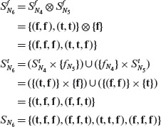
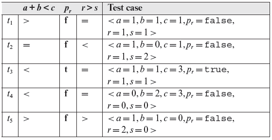
4
Predicate Analysis
CONTENTS
The purpose of this chapter is to introduce techniques for the generation of test data from requirements specified using predicates. Such predicates are extracted either from the informally or formally specified requirements or directly from the program under test. There exist a variety of techniques to use one or more predicates as input and generate tests. Some of these techniques can be automated while others may require significant manual effort for large applications. It is not possible to categorize such techniques as either black or white box technique. Depending on how the predicates are extracted, a technique could be termed as a black or white box technique.
4.1 Introduction
The focus of this chapter is the generation of tests from informal as well as rigorously specified requirements. These requirements serve as a source for the identification of the input domain of the application to be developed. A variety of test generation techniques are available to select a subset of the input domain to serve as test set against which the application will be tested.
Figure 3.1 lists some techniques described in this chapter. The figure shows requirements specification in three forms: informal, rigorous, and formal. The input domain is derived from the informal and rigorous specifications. The input domain then serves as a source for test selection. Various techniques, listed in the figure, are used to select a relatively small number of test cases from a usually very large input domain.
4.2 Domain Testing
Path domains and domain errors have been introduced in Chapter 2. Recall that a program contains a domain error if on an input it follows an incorrect path due to incorrect condition or incorrect computation. Domain testing is a technique for generating tests to detect domain errors. The technique is similar to boundary value analysis discussed earlier. However in domain testing, the requirements for test generation are extracted from the code. Hence domain testing could also be considered as a white-box testing technique. While domain testing is also an input domain partitioning technique, it is included in this chapter due to its focus on predicate analysis.
Domain testing aims at selecting tests from the input domain to detect any domain errors. A domain error is said to occur when an incorrect path leads to an incorrect or a correct path leads an incorrect output.
4.2.1 Domain errors
As mentioned earlier, a path condition consists of a set of predicates that occur along the path in a conditional or a loop statement. A path condition gives rise to a path domain that has a boundary. The boundary consists of one or more border segments, also known as borders. There is one border corresponding to each predicate in the path condition. An error in any of the predicates in a path condition leads to a change in the boundary due to border shift. It is such border shifts, probably unintended, the determination of which is the target of domain testing.
Every path in a program has a condition associated with it. This condition is known as a path condition and must hold for the path to be traversed.
Considering only linear predicates without any Boolean conditions such as AND and OR, the boundary and its borders can be shown as in Figure 4.1. The figure shows three types of domain errors corresponding to the correct path domain in Figure 4.1(a). A border shift occurs as shown in Figure 4.1(b) and (c). The border shift in Figure 4.1(b) is parallel whereas in Figure 4.1(c) it is tilted. The method described here does not depend on the kind of border shift. Figure 4.1(d) shows an extra border corresponding to the condition y < 0.5. Figure 4.1(e) shows a missing border due to a missing condition y < x + 1.
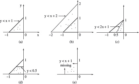
Figure 4.1 Types of domain errors. (a) Correct boundary corresponding to the path condition y < x + 1 ∧ y > 0 ∧ x < 0. (b) and (c) Boundary shifted due to error in y < x + 1. (d) Extra border due to the inclusion of y < 0.5 in the path condition. (e) Missing border due to missing y < x + 1. The dots indicate points inside the boundary.
4.2.2 Border shifts
As mentioned earlier, and illustrated in Figure 4.1, a domain error occurs due to a possibly unintended shift in the border. Thus, the idea underlying domain testing is to sample points inside and outside the displaced area in the hope that the error would be detected. This idea is independent of whether or not a border is linear or non-linear.
A border shift occurs due to an incorrect condition. The shift refers to a change in the boundary of path domain due to an error in the coding of the path condition.
As we now know, in the case of linear constraints in two dimensions, a path domain is specified by a set of one or more straight line borders. A border is a line corresponding to a simple predicate. A border that corresponds to a predicate using any of the operators ≤,≥, and =, is considered closed. Thus, points that lie on a closed border are part of the path domain. A border that corresponds to a predicate using any of the operators <, > or ≠ is considered open. Points that lie on the open border are not part of the path domain.
Note that a border is always defined using equality. However, whether or not points defined by a predicate lie in or out of the path domain is determined by the actual relational operator in the predicate. For example, the predicate y – x < 0 defines an open border. Hence all points that satisfy the relation y – x = 0 are not included in the path domain while those that satisfy the inequality are. However, for a predicate y – x ≤ 0, all points that satisfy the equality are included in the path domain.
4.2.3 ON-OFF points
Testing for boundary shifts is done with the help of ON and OFF points. An ON point must satisfy the path condition associated with the border. It need not be exactly on the given border but should be near. An OFF point must be as close as possible to the ON point for that border. It lies outside the border and hence does not satisfy the condition associated with the border.
An ON point occurs on or near a boundary. An OFF point is close to an OFF point but lies outside the border and does not satisfy the path condition.
While testing for a boundary shift error, only one ON and one OFF point is needed for inequality constraints. For an equality (=) or non-equality (≠) constraint one ON point and two OFF points are selected; the OFF points lie on the opposite sides of the border. The following examples illustrate the selection of ON and OFF points and the detection of domain errors.
The number of ON and OFF points needed to test a path condition depends on whether an equality or an inequality constraint occurs in the condition.
Example 4.1 Consider the following contrived function ƒ that we assume to be incorrect. The two domain errors in ƒ are indicated alongside the erroneous statements. Depending on the inputs ƒ displays a string consisting of a sequence of integers from 1 through 4. The displayed sequence depends on the values of its input parameters x and y.
1 String f (int x, int y){
2 String s=" ";
3 if(y<x+1) // Error 1: this should be y < x + 2
4 s=s+"1";
5 if(y>0)
6 s=s+"2";
7 if(x<=0) // Error 2: this should be x < y
8 s=s+"3";
9 s=s+"4";
10 return s;
11 }
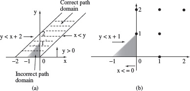
For the sake of simplicity let us consider the following path p through function ƒ : 1, 2, 3, 4, 5, 6, 7 , 9, 10. The path condition c is y < x + 1 ∧ y > 0 ∧ x ≤ 0. Given that ƒ has two errors, the correct path condition c′ is y < x + 2 ∧ y > 0 ∧ x < y. Figure 4.2(a) shows the path domains corresponding to c and c′. The shaded area in the figure denotes the incorrect path domain while the dashed area the correct one. Generation of tests for the path condition proceeds as follows.
ON and OFF points are generated for each simple predicate in a path condition. It is best to avoid the reuse of points.
- Generate ON and OFF points for each predicate in the path condition. It is best to avoid the reuse of points to increase chances of finding errors.
- For each point determine the expected value of the program under test. Each point, together with the expected output, constitutes a test case.
- Run the program under test on each test case and determine if the actual output is the same as the expected output.
Figure 4.2(b) shows a scaled version of the incorrect path domain and the corresponding ON and OFF points. Given that x and y are integers, the shaded area is empty in the sense that there are no points inside this area.
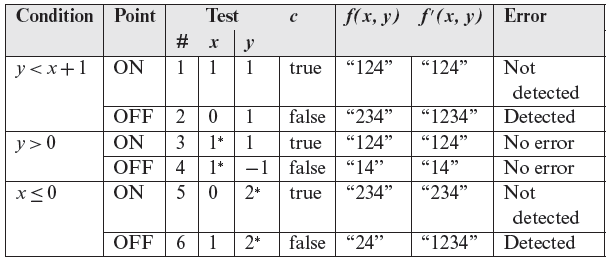
The following table lists the outcome of generating the ON and OFF points and executing ƒ against these tests. In the table ƒ denotes the function under test and ƒ′ the correct function. Obviously, ƒ′ is not known during testing. However, we assume it is possible to determine the expected output f′(x, y), from the requirements.
Figure 4.2 (a) Path domains corresponding to the incorrect and correct path conditions in Example 4.1. (b) Incorrect path domain, scaled up, and the ON-OFF points.
*Any value will satisfy the requirement imposed by the point type.
The rightmost three columns in the above table show the outcome of executing ƒ against the four tests and the expected outcome. Note that in this case both errors are detected by the OFF points.
The above example is simple and used for illustrating how tests are determined using the ON and OFF points. Notice that all conditions along a path are independent in the sense that the outcome of a condition does not depend on that of any other condition. In practice, this may not be true. Exercise 4.1 illustrates dependent predicates in a path condition.
A path condition might contain simple conditions that depend on each other. In such cases it is best to simplify the path condition prior to the generation ƒ ON and OFF points so that the revised path condition consists of independent simple conditions. Of course the original and the new conditions must be semantically equivalent.
Example 4.2 Suppose that the predicate x==y defines a border in a path domain for integer inputs x and y. This is an equality border and we need one ON and two OFF points. Following are the test cases for testing any border shift corresponding to this border.
ON: (x=1, y=1)
OFF1: (x=1, y=2)
OFF2: (x=2, y=1)
Note that the two OFF points are on the opposite sides of the border and close to the ON point. Now suppose that the correct border is defined by the condition x==y+1. In this case, the test cases corresponding to the ON and OFF2 points lead to different outcomes for the two conditions. For any other equality, the ON point leads to different outcomes for the two conditions.
4.2.4 Undetected errors
Domain testing as described above is not guaranteed to detect errors due to shifted boundaries. An error might go undetected when the correct boundary lies between the incorrect boundary and the OFF point. The next example illustrates such a situation.
An error might go undetected when the correct boundary lies between the two incorrect boundaries.
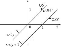
Example 4.3 Suppose that the incorrect path condition in the following function is x < y. The correct condition is assumed to be x < y + 1.
1
2 int f (double x, double y){
3 if (x<y) // Correct condition is x < y + 1
4 return 1;
5 else
6 return 2;
7 }
One possible set of ON and OFF points derived from the incorrect condition are: ON: (x = 1, y = 1.001) and OFF: (x = 1.5, y = 0.4). Note that, as required, the ON point satisfies the border condition and is close to the border. Again, as required, the OFF point does not satisfy the border condition. However, the OFF point is not close to the ON point.
For both test cases, the correct and the incorrect path conditions evaluate to the same truth values and hence the error goes undetected. As shown in Figure 4.3, the correct border corresponding to x < y + 1 passes between the incorrect border and the OFF point.
Figure 4.3 Path domains corresponding x < y (incorrect) and x < y + 1 (correct). ON and OFF points shown do not detect the error. Note that the correct border lies between the incorrect border and the OFF point. OFF′ point does detect the error as it lies between the incorrect and the correct borders (see Example 4.3.)
Now suppose we select the OFF point very near the incorrect border, as it should have been. Thus, for example, OFF: (x = 1, y = 0.999). In this case, the OFF point lies between the correct and the incorrect borders. The error is now detected because the incorrect condition evaluates to false but the correct condition evaluates to true.
4.2.5 Coincidental correctness
Coincidental correctness may also cause an error to go undetected. This happens when the expected and the actual outcomes of executing a program match despite a program error.
Coincidental correctness occurs when the expected and the actual output of a program match despite the execution of an incorrect path.
Example 4.4 Consider the following function.
1 int f (int z){
2 if (z>15) // Error: The condition should be z>=15.
3 return z-10;
4 else
5 return z%10;
6 }
Now suppose that the function above is invoked with the value of z as 15. In this case, the function would return 5 regardless of whether the path condition is as given or the correct one. Thus, the error is not revealed. Notice that the error is revealed by several other values of z, for example, for z = 5. Also see Exercise 4.19 for another example.
4.2.6 Paths to be tested
The generation of tests using domain testing starts with the selection of a path. The path selected then determines the predicates that lie on it and hence the path domain. A tester may select a path based on a variety of criteria. For example, there might be a path that is considered critical to the application under test. This could become a selected path.
Most programs have an exorbitantly large number of paths. A tester needs to decide one or more suitable criteria to select which of the many paths are to be tested.
In general, one needs to pick a suitable criterion to decide what paths to select. Several useful criteria are introduced in Chapter 7. As an example, one could use the boundary-interior coverage criterion. The selected paths must start from the beginning of the program and ensure that each loop is executed zero times along one path and once along the other. The execution of the body zero times corresponds to the boundary condition. The execution of the body once corresponds to the interior condition. In some cases only one selected path might satisfy the condition though it is likely that at least two will be needed.
4.3 Cause-Effect Graphing
We described two techniques for test selection based on equivalence partitioning and boundary value analysis. One is based on unidimensional partitioning and the other on multidimensional partitioning of the input domain. While equivalence classes created using multidimensional partitioning allow the selection of a large number of input combinations, the number of such combinations could be astronomical. Further, many of these combinations, as in Example 4.8, are infeasible and make the test selection process tedious.
Cause-effect graphing is a visual technique for modeling the relationships between inputs and output of a program. The inputs (cases) could be specified as conditions and the output (effects) in terms of expected values or behavior.
Cause-effect graphing, also known as dependency modeling, focuses on modeling dependency relationships amongst program input conditions, known as causes, and output conditions, known as effects. The relationship is expressed visually in terms of a cause-effect graph. The graph is a visual representation of a logical relationship amongst inputs and outputs that can be expressed as a Boolean expression. The graph allows selection of various combinations of input values as tests. The combinatorial explosion in the number of tests is avoided by using certain heuristics during test generation.
A cause is any condition in the requirements that may effect the program output. An effect is the response of the program to some combination of input conditions. It may be, for example, an error message displayed on the screen, a new window displayed, or a database updated. An effect need not be an “output” visible to the user of the program. Instead, it could also be an internal test point in the program that can be probed during testing to check if some intermediate result is as expected. For example, the intermediate test point could be at the entrance into a method to indicate that indeed the method has been invoked.
A requirement such as “Dispense food only when the DF switch is ON” contains a cause “DF switch is ON” and an effect “Dispense food.” This requirement implies a relationship between the “DF switch is ON” and the effect “Dispense food.” Of course, other requirements might require additional causes for the occurrence of the “Dispense food” effect. The following generic procedure is used for the generation of tests using cause-effect graphing.
- Identify causes and effects by reading the requirements. Each cause and effect is assigned a unique identifier. Note that an effect can also be a cause for some other effect.
- Express the relationship between causes and effects using a cause-effect graph.
- Transform the cause-effect graph into a limited entry decision table, hereafter referred to simply as decision table.
- Generate tests from the decision table.
The basic notation used in cause-effect graphing and a few illustrative examples follow.
4.3.1 Notation used in cause-effect graphing
The basic elements of a cause-effect graph are shown in Figure 4.4. A typical cause-effect graph is formed by combining the basic elements so as to capture the relations between causes and effects derived from the requirements. The semantics of the four basic elements shown in Figure 4.4 is expressed below in terms of the if-then construct; C, C1, C2, and C3 denote causes and Ef denotes an effect.
Figure 4.4 Basic elements of a cause-effect graph: implication, not (~), and (∧), or (∨). C, C1, C2, and C3 denote causes and Ef denotes effect. An arc is used, for example in the and relationship, to group three or more causes.
|
C implies Ef : |
if (C) then Ef ; |
|
not C implies Ef : |
if (¬C) then Ef ; |
|
Ef when C1 and C2 and C3 : |
if (C1 && C2 && C3) then Ef ; |
|
Ef when C1 or C2 : |
if (C1 ǁ C2) then Ef ; |
There often arise constraints amongst causes. For example, consider an inventory control system that tracks the inventory of various items that are stocked. For each item, an inventory attribute is set to “Normal,” “Low,” and “Empty.” The inventory control software takes actions as the value of this attribute changes. When identifying causes, each of the three inventory levels will lead to a different cause listed below.
Constraints among conditions (effects) can be specified in a cause-effect graph.
Constraints among causes are Ε (Exclusive), I (inclusive), R (required), and Ο (one and only one). These constraints, except R, are n-ary meaning that they hold among two or more causes. The R constraint is considered binary.
C1 : “Inventory is normal”
C2 : “Inventory is low”
C3 : “Inventory is zero”
However, at any instant, exactly one of C1, C2, C3 can be true. This relationship amongst the three causes is expressed in a cause-effect graph using the “Exclusive (E)” constraint shown in Figure 4.5. In addition, shown in this figure are the “Inclusive (I),” “Requires (R),” and “One and only one (O),” constraints. The I constraint between two causes C1 and C2 implies that at least one of the two must be present. The R constraint between C1 and C2 implies that C1 requires C2. The Ο constraint models the condition that one, and only one, of C1 and C2 must hold.
Figure 4.5 Constraints amongst causes (E, I, O, and R).
The table below lists all possible values of causes constrained by Ε, I, R, and O. A 0 or a 1 under a cause implies that the corresponding condition is, respectively, false and true. The arity of all constraints, except R, is greater than 1, i.e., all except the R constraint can be applied to two or more causes; the R constraint is applied to two causes.
In addition to the constraints on causes, there could also be constraints on effects. The cause-effect graphing technique offers one constraint, known as “Masking (M)” on effects. Figure 4.6 shows the graphical notation for the masking constraint. Consider the following two effects in the inventory example mentioned earlier.

Figure 4.6 The masking constraint amongst effects.
Constraints could also be specified among the effects. One such constraint is Μ (masking) that indicates that a given effect masks another.
Eƒ1: Generate “Shipping invoice.”
Eƒ2: Generate an “Order not shipped” regret letter.
Effect Eƒ1 occurs when an order can be met from the inventory. Effect Eƒ2 occurs when the order placed cannot be met from the inventory or when the ordered item has been discontinued after the order was placed. However, Eƒ2 is masked by Eƒ1 for the same order, i.e. both effects cannot occur for the same order.
A condition that is false (true) is said to be in the “0 state” (1 state). Similarly, an effect can be “present” (1 state) or “absent” (0 state).
4.3.2 Creating cause-effect graphs
The process of creating a cause-effect graph consists of two major steps. First, the causes and effects are identified by a careful examination of the requirements. This process also exposes the relationships amongst various causes and effects as well as constraints amongst the causes and effects. Each cause and effect is assigned a unique identifier for ease of reference in the cause-effect graph.
A cause-effect graph is derived from causes and effects derived from the requirements.
In the second step, the cause-effect graph is constructed to express the relationships extracted from the requirements. When the number of causes and effects is large, say over 100 causes and 45 effects, it is appropriate to use an incremental approach. An illustrative example follows.
Example 4.5 Let us consider the task of test generation for a GUI based computer purchase system. A web-based company is selling computers (CPU), printers (PR), monitors (M), and additional memory (RAM). An order configuration consists of one to four items as shown in Figure 4.7. The GUI consists of four windows for displaying selections from CPU, Printer, Monitor, and RAM and one window where any free giveaway items are displayed.
Figure 4.7 Possible configurations of a computer system sold by a web-based company. CPU: CPU configuration, PR: Printer, M: Monitor. RAM: memory upgrade.
For each order, the buyer may select from three CPU models, two printer models, and three monitors. There are separate windows one each for CPU, printer, and monitor that show the possible selections. For simplicity we assume that RAM is available only as an upgrade and that only one unit of each item can be purchased in one order.
Monitors Μ 20 and Μ 23 can be purchased with any CPU or as a stand-alone item. Μ 30 can only be purchased with CPU 3. PR 1 is available free with the purchase of CPU 2 or CPU 3. Monitors and printers, except for Μ 30, can also be purchased separately without purchasing any CPU. Purchase of CPU 1 gets RAM 256 upgrade, purchase of CPU 2 or CPU 3 gets a RAM 512 upgrade. The RAM 1G upgrade and a free PR 2 is available when CPU 3 is purchased with monitor Μ 30.
When a buyer selects a CPU, the contents of the printer and monitor windows are updated. Similarly, if a printer or a monitor is selected, contents of various windows are updated. Any free printer and RAM available with the CPU selection is displayed in a different window marked “Free.” The total price, including taxes, for the items purchased is calculated and displayed in the “Price” window. Selection of a monitor could also change the items displayed in the “Free” window. Sample configurations and contents of the “Free” window are given below.
Items purchased
“Free” window
Price
CPU 1
RAM 256
$499
CPU 1. PR 1
RAM 256
$628
CPU 2. PR 2. M23
PR 1, RAM 512
$2257
CPU 3. M30
PR 2, RAM 1G
$3548
The first step in cause-effect graphing is to read the requirements carefully and make a list of causes and effects. For this example, we will consider only a subset of the effects and leave the remaining as an exercise. This strategy also illustrates how one could generate tests using an incremental strategy.
A cause in a cause-effect graph could be a condition such as “Purchase an item” or “Deposit money”. An effect could be, for example, “Print invoice” or “Update account balance.” An effect could become a cause for another effect.
A careful reading of the requirements is used to extract the following causes. We have assigned a unique identifier, C1 through C8 to each cause. Each cause listed below is a condition that can be true or false. For example, C8 is true if monitor Μ 30 is purchased.
C1 : Purchase CPU 1.
C2 : Purchase CPU 2.
C3 : Purchase CPU 3.
C4 : Purchase PR 1.
C5 : Purchase PR 2.
C6 : Purchase M 20.
C7 : Purchase M 23.
C8 : Purchase M 30.
Note that while it is possible to order any of the items listed above, the GUI will update the selection available depending on which CPU, or any other item, is selected. For example, if CPU 3 is selected for purchase then monitors Μ 20 and Μ 23 will not be available in the monitor selection window. Similarly, if monitor Μ 30 is selected for purchase, then CPU 1 and CPU 2 will not be available in the CPU window.
Next, we identify the effects. In this example, the application software calculates and displays the list of items available free with the purchase and the total price. Hence the effect is in terms of the contents of the “Free” and “Price” windows. There are several other effects related to the GUI update actions. These effects are left for the exercise (see Exercise 4.4).
Calculation of the total purchase price depends on the items purchased and the unit price of each item. The unit price is obtained by the application from a price database. The price calculation and display is a cause that creates the effect of displaying the total price. For simplicity, we ignore the price related cause and effect. The set of effects in terms of the contents of the “Free” display window are listed below.
Eƒ1 : RAM 256.
Eƒ2 : RAM 512 and PR 1.
Eƒ3 : RAM 1G and PR 2.
Eƒ4 : No giveaway with this item.
Now that the causes, effects, and their relationships have been identified, we can begin to construct the cause-effect graph. Figure 4.8 shows the complete graph that expresses the relationships between C1 through C8 and effects Eƒ1 through Ef4.
Once the conditions (causes) and the expected outcome (effects) have been identified, the relationship amongst them can be expressed using a cause-effect graph.
From the cause-effect graph in Figure 4.8 we notice that C1, C2, and C3 are constrained using the Ε (exclusive) relationship. This expresses the requirement that only one CPU can be purchased in one order. Similarly, C3 and C8 are related via the R (requires) constraint to express the requirement that monitor Μ 30 can only be purchased with CPU 3. Relationships amongst causes and effects are expressed using the basic elements shown earlier in Figure 4.4.
Notice the use of an intermediate node labeled 1 in Figure 4.8. Though not necessary in this example, such intermediate nodes are often useful when an effect depends on conditions combined using more than one operator, for example, (C1 ∧ C2) ∨ C3. Note also that purchase of printers and monitors without any CPU leads to no free item (Ef4).
The relationships between effects and causes shown in Figure 4.8 can be expressed in terms of Boolean expressions as follows:
Figure 4.8 Cause-effect graph for the web-based computer sale application. C1, C2, and C3 denote the purchase of, respectively, CPU 1, CPU 2, and CPU 3. C4 and C5 denote the purchase of printers PR 1 and PR 2, respectively. C6, C7, and C8 denote the purchase of monitors Μ 20, Μ 23, and Μ 30, respectively.
Eƒ1 = C1
Eƒ2 = C2 ∨ C3
Eƒ3 = C3 ∧ C8
Eƒ4 = C4 ∧ C5 ∧ C6 ∧ C7
4.3.3 Decision table from cause-effect graph
We will now see how to construct a decision table from a cause-effect graph. Each column of the decision table represents a combination of input values, and hence a test. There is one row for each condition and effect. Thus the decision table can be viewed as an N × Μ matrix with Ν being the sum of the number of conditions and effects and Μ the number of tests.
A decision table is a tabular representation of a cause-effect graph. It makes it easy to generate tests.
Each entry in the decision table is a 0 or a 1 depending on whether or not the corresponding condition is false or true, respectively. For a row corresponding to an effect, an entry is 0 or 1 if the effect is not present or present, respectively. Following is a procedure to generate a decision table from a cause-effect graph.
Procedure for generating a decision table from a cause-effect graph.
|
Input: |
A cause-effect graph containing causes C1, C2,…, Cp and effects Eƒ1, Eƒ2, … ,Eƒq. |
|
A decision table DT containing N = p + q rows and Μ columns, where Μ depends on the relationship between the causes and effects as captured in the cause-effect graph. |
Procedure: CEGDT
|
/* |
i is the index of the next effect to be considered. |
|
|
next_dt_col is the next empty column in the decision table. |
|
|
Vk: a vector of size p + q containing 1’s and 0’s. Vj, 1 ≤ j ≤ p, indicates the state of condition Cj and Vl, p < l ≤ p + q, indicates the presence or absence of effect Efl–p. |
|
*/ |
|
|
Step 1 |
Initialize DT to an empty decision able. |
|
|
next_dt_col = 1. |
|
Step 2 |
Execute the following steps for i = 1 to q. |
|
2.1 |
Select the next effect to be processed. |
|
|
Let e = Efi. |
|
2.2 |
Find combinations of conditions that cause e to be present. |
|
|
Assume that e is present. Starting at e, trace the cause-effect graph backwards and determine the combinations of conditions C1, C2, . . .,Cp that lead to e being present. Avoid combinatorial explosion by using the heuristics given in the text following this procedure. Make sure that the combinations satisfy any constraints amongst the causes. |
|
|
Let V1, V2, …, Vmi be the combinations of causes that lead to e being present. There must be at least one combination that makes e to be present, i.e. in 1 state, and hence mi≥ 1. Set Vk(l), p < l ≤ p + q to 0 or 1 depending on whether effect Efl–p is present or not for the combination of all conditions in Vk. |
|
2.3 |
Update the decision table. |
|
|
Add V1, V2,…,Vmi to the decision table as successive columns starting at next_dt_col. |
|
2.4 |
Update the next available column in the decision table. |
|
|
next_dt_col = next_dt_col + mi. At the end of this procedure, next_dt_col – 1 is the number of tests generated. |
End of Procedure CEGDT
Determination of a combination of conditions that lead to the presence of an effect is done by tracing backwards in the cause-effect starting at an effect and stopping when the truth values of all relevant conditions have been determined.
Procedure CEGDT can be automated for the generation of tests. However, as indicated in Step 2.2, one needs to use some heuristics in order to avoid combinatorial explosion in the number of tests generated. Before we introduce the heuristics, we illustrate through a simple example the application of procedure CEGDT without applying the heuristics in Step 2.
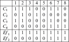
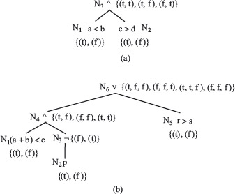
Example 4.6 Consider the cause-effect graph in Figure 4.9. It shows four causes labeled d,C1, C2, C3, and C4 and two effects labeled Ef1 and Ef2. There are three intermediate nodes labeled 1, 2, and 3. Let us now follow procedure CEGDT step-by-step to generate a decision table.
In Step 1 we set next_dt_col = 1 to initialize the decision table to empty. Next, i = 1 and, in accordance with Step 2.1, e = Ef1 Continuing further and in accordance with Step 2.2, trace backwards from e to determine combinations that will cause e to be present. e must be present when node 2 is in 1-state. Moving backwards from node 2 in the cause-effect graph, note that any of the following three combinations of states of nodes 1 and C3 will lead to e being present: (0, 1), (1, 1), and (0, 0).
Node 1 is also an internal node and hence move further back to obtain the values of C1 and C2 that effect node 1. Combination of C1 and C2 that brings node 1 to the 1-state is (1, 1) and combinations that bring it to 0-state are (1, 0), (0, 1), and (0, 0). Combining this information with that derived earlier for nodes 1 and C3, we obtain the following seven combinations of C1, C2, and C3 that cause e to be present.
1 0 1
0 1 1
0 0 1
Figure 4.9 A cause-effect graph to illustrate procedure CEGDT.
1 0 0
0 1 0
0 0 0
Next, from Figure 4.9, note that C3 requires C1 which implies that C1 must be in 1-state for C3 to be in 1-state. This constraint makes infeasible the second and third combinations above. In the end, we obtain the following five combinations of the four causes that lead to e being present.
1 0 1
1 1 1
1 0 0
0 1 0
0 0 0
Setting C4 to 0 and appending the values of Efl and Ef2, we obtain the following five vectors. Note that m1 = 5 in Step 2. This completes the application of Step 2.2, without the application of any heuristics, in the CEGDT procedure.
V1 1 0 1 0 1 0
V2 1 1 1 0 1 0
V3 1 0 0 0 1 0
V4 0 1 0 0 1 0
V5 0 0 0 0 1 0
The five vectors are transposed and added to the decision table starting at column next_dt_col which is 1. The decision table at the end of Step 2.3 follows.
We update next_dt_col to 6, increment i to 2 and get back to Step 2.1. We now have e = Ef2. Tracing backwards, we find that for e to be present, node 3 must be in the 1-state. This is possible with only one combination of node 2 and C4, which is (1, 1).
Earlier we derived the combinations of C1, C2, and C3 that lead node 2 into the 1-state. Combining these with the value of C4 we arrive at the following combination of causes that lead to the presence of Ef2.
1 0 1 1
1 1 1 1
1 0 0 1
0 1 0 1
0 0 0 1
From Figure 4.9 we note that C2 and C4 cannot be present simultaneously. Hence, we discard the second and the fourth combinations from the list above and obtain the following three feasible combinations.
1 0 1 1
1 0 0 1
0 0 0 1
Appending the corresponding values of Ef1 and Ef2 to each of the above combinations, we obtain the following three vectors.
V1 1 0 1 1 1 1
V2 1 0 0 1 1 1
V3 0 0 0 1 1 1
Transposing the vectors listed above and appending them as three columns to the existing decision table, we obtain the following.
Next we update nxt_dt_col to 9. Of course, doing so is useless as the loop set up in Step 2 is now terminated. The decision table listed above is the output obtained by applying procedure CEGDT to the cause-effect graph in Figure 4.9.
4.3.4 Heuristics to avoid combinatorial explosion
While tracing back through a cause-effect graph we generate combinations of causes that set an intermediate node, or an effect, to a 0 or a 1 state. Doing so in a brute force manner could lead to a large number of combinations. In the worst case, if n causes are related to an effect e, then the maximum number of combinations that bring e to a 1-state is 2n.
A brute force method to determine conditions that will cause an effect to be present will likely generate a large number of tests. A few simple heuristics can be used to avoid a combinatorial explosion.
As tests are derived from the combinations of causes, large values of n could lead to an exorbitantly large number of tests. We avoid such a combinatorial explosion by using simple heuristics related to the “AND” (∧) and “OR” (∨) nodes.
Certainly, the heuristics described below are based on the assumption that certain types of errors are less likely to occur than others. Thus, while applying the heuristics to generate test inputs will likely lead to a significant reduction in the number of tests generated, it may also discard tests that would have revealed a program error. Hence, one must apply the heuristics with care and only when the number of tests generated without their application is too large to be useful in practice.
While the application of heuristics will likely reduce the number of tests, it might also reduce the error detection effectiveness of the generated test suite.
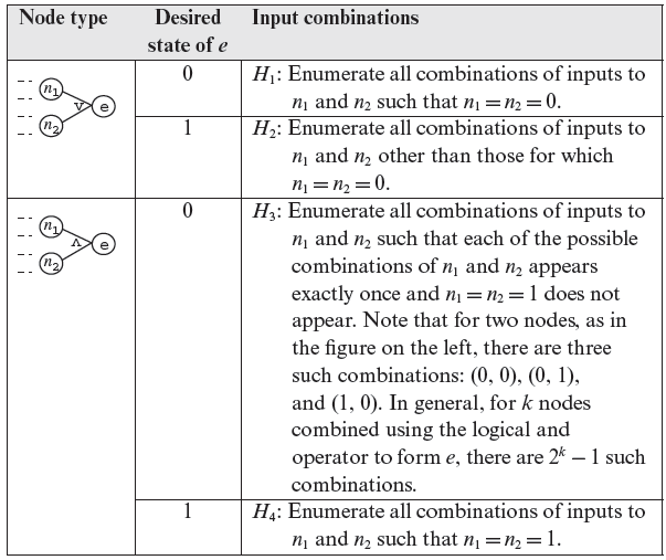
A set of four heuristics labeled H1 through H4, is given in Table 4.1. The leftmost column shows the node type in the cause-effect graph, the center column is the desired state of the dependent node, and the rightmost column is the heuristic for generating combinations of inputs to the nodes that effect the dependent node e.
For simplicity we have shown only two nodes n1 and n2 and the corresponding effect e; in general there could be one or more nodes related to e. Also, each of n1 and n2 might represent a cause or may be an internal node with inputs, shown as dashed lines, from causes or other internal nodes. The next example illustrates the application of the four heuristics shown in Table 4.1.
Table 4.1 Heuristics used during the generation of input combinations from a cause-effect graph.
Example 4.7 Consider the cause-effect graph in Figure 4.10. We have at least two choices while tracing backwards to derive the necessary combinations: derive all combinations first and then apply the heuristics and derive combinations while applying the heuristics. Let us opt for the first alternative as it is a bit simple to use in this example.
Figure 4.10 Cause-effect graph for Example 4.7.
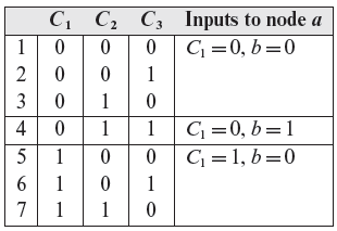
Suppose that we require node e to be 1. Tracing backwards, this requirement implies that node a must be a 0. If we trace backwards further, without applying any heuristic, we obtain the following seven combinations of causes that bring e to 1 state. The last column lists the inputs to node a. The combinations that correspond to the inputs to node a listed in the rightmost column are separated by horizontal lines.
One may apply the heuristics while generating the conditions for an effect to be present or not present. Alternately one may first generate the conditions using a brute force method and then apply the heuristics to remove the undesirable conditions as shown here.
Let us now generate tests using the heuristics applicable to this example. First we note that node a matches the OR-node shown in the top half of Table 4.1. As we want the state of node a to be 0, heuristic H1 applies in this situation. H1 asks us to enumerate all combinations of inputs to node a such that C1 and node b are 0. (0, 0) is the only such combination and is listed in the last column of the following table.
Let us begin with (0, 0). No heuristic applies to C1 as it has no preceding nodes. Node b is an AND-node as shown in the bottom half of Table 4.1. We want node b to be 0 and therefore H3 applies. In accordance with H3 we generate three combinations of inputs to node b: (0, 0), (0, 1), and (1, 0). Notice that combination (1, 1) is forbidden. Joining these combinations of C2 and C3 with C1 = 0, we obtain the first three combinations listed in the preceding table.
Though not required here, suppose that we were to consider the combination C1 = 0,b = 1. Heuristic H4 applies in this situation. As both C2 and C3 are causes with no preceding nodes, the only combination we obtain now is (1, 1). Combining this with C1 = 0 we obtain sequence 4 listed in the preceding table.
We have completed the derivation of combinations using the heuristics listed in Table 4.1. Note that the combinations listed above for C1 = 1, b = 0 are not required. Thus, we have obtained only three combinations instead of the seven enumerated earlier. The reduced set of combinations is listed below.
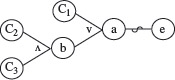
Let us now examine the rationale underlying the various heuristics for reducing the number of combinations. Heuristic H1 does not save us on any combinations. The only way an OR-node can cause its effect e to be 0 is for all its inputs to be 0. H1 suggests that we enumerate all such combinations. Heuristic H2 suggests that we use all combinations that cause e to be 1 except those that cause n1 = n2 = 0. To understand the rationale underlying H2 consider a program required to generate an error message when condition c1 or c2 is true. A correct implementation of this requirement is given below.
if(c1 ∨ c2) print(“Error”);
Application of a heuristic may or may not save on tests.
Now consider the following erroneous implementation of the same requirement.
if(c1 ∨ ¬c2) print(“Error”);
A test that sets both c1 and c2 true will not be able to detect an error in the implementation above if short circuit evaluation is used for Boolean expressions. However, a test that sets c1= 0 and c2 = 1 will be able to detect this error. Hence H2 saves us from generating all input combinations that generate the pair (1, 1) entering an effect in an OR-node (see Exercise 4.6).
Heuristics H3 saves us from repeating the combinations of n1 and n2. Once again this could save us a lot of tests. The assumption here is that any error in the implementation of e will be detected by tests that cover different combinations of n1 and n2. Thus, there is no need to have two or more tests that contain the same combination of n1 and n2.
Lastly, H4 for the AND-node is analogous to H1 for the OR-node. The only way an AND-node can cause its effect e to be 1 is for all its inputs to be 1. H4 suggests that we enumerate all such combinations. We stress, once again, that while the heuristics discussed above will likely reduce the set of tests generated using cause-effect graphing, they might also lead to useful tests being discarded. Of course, in general and prior to the start of testing, it is almost impossible to know which of the test cases discarded will be useless and which ones useful.
4.3.5 Test generation from a decision table
Test generation from a decision table is relatively straightforward. Each column in the decision table generates at least one test input. Note that each combination might be able to generate more than one test when a condition in the cause-effect graph can be satisfied in more than one way. For example, consider the following cause:
C: x < 99.
Tests are generated from the decision table obtain from a cause-effect graph. Each combination of conditions may generate more than one test case.
The condition above can be satisfied by many values such as x = 1, and x = 49. Also, C can be made false by many values of x such as x = 100 and x = 999. Thus, one might have a choice of values of input variables while generating tests using columns from a decision table.
While one could always select values arbitrarily as long as they satisfy the requirement in the decision table, it is recommended that the choice be made so that tests generated are different from those that may have already been generated using some other technique such as, for example, boundary value analysis. Exercise 4.8 asks you to develop tests for the GUI-based computer purchase system in Example 4.5.
4.4 Tests Using Predicate Syntax
In this section, we introduce techniques for generating tests that are aimed at detecting faults in the coding of conditions. The conditions from which tests are generated might arise from requirements or might be embedded in the program to be tested.
Cause-effect graphing is a visual method for capturing the requirements and then generating tests. Another way to generate tests from predicates, which are conditions in a cause-effect graph, is to use abstract syntax trees as a representation of a predicate. The syntax tree is then used to derive tests using one of three procedures described here.
A condition is represented formally as a predicate. For example, consider the requirement “if the printer is ON and has paper then send the document for printing.” This statement consists of a condition part and an action part. The following predicate, denoted as pr, represents the condition part of the statement.
pr: (printer_status=ON) ∧ (printer_tray= ¬ empty)
The predicate pr consists of two relational expressions joined with the ∧ Boolean operator. Each of the two relational expressions uses the equality (=) symbol. A programmer might code pr correctly or might make an error thus creating a fault in the program. We are interested in generating test cases from predicates such that any fault, that belongs to a class of faults, is guaranteed to be detected during testing. Testing to ensure that there are no errors in the implementation of predicates is also known as predicate testing.
We begin our move towards the test generation algorithm by first defining some basic terms related to predicates and Boolean expressions. Then we will examine the fault model that indicates what faults are the targets of the tests generated by the algorithms presented. This is followed by an introduction to constraints and tests and then the algorithm for which you would have waited so long.
4.4.1 A fault model
Predicate testing, as introduced in this chapter, targets three classes of faults: Boolean operator fault, relational operator fault, and arithmetic expression fault. A Boolean operator fault is caused when (i) an incorrect Boolean operator is used, (ii) a negation is missing or placed incorrectly, (iii) parentheses are incorrectly placed, and (iv) an incorrect Boolean variable is used. A relational operator fault occurs when an incorrect relational operator is used. An arithmetic expression fault occurs when the value of an arithmetic expression is off by an amount equal to ϵ.
Predicate testing is useful in detecting errors in the use of Boolean and relational operators as well as off-by-1 errors in arithmetic expressions used in a condition.
Given a predicate pr and a test case t, we write p(t) as an abbreviation for the truth value obtained by evaluating pr on t. For example, if pr is a < b ∧ r > s and t is < a = 1, b = 2, r = 0, s = 4 >, then p(t) = false. Let us now examine a few examples of the faults in the fault model used in this section.
Boolean operator fault: Suppose that the specification of a software module requires action to be performed when the condition (a < b) ∨ (c > d) ∧ e is true. Here a, b, c, and d are integer variables and e a Boolean variable. Three incorrect codings of this condition, each containing a Boolean operator fault, are given below.
|
(a < b)∧(c > d)∧e |
Incorrect Boolean operator |
|
(a < b)∨¬(c > d)∧e |
Incorrect negation operator |
|
(a < b)∧(c > d)∨e |
Incorrect Boolean operators |
|
(a < b)∨(c > d)∧f |
Incorrect Boolean variable (f instead of e). |
The incorrect use of a Boolean operator is known as a Boolean operator fault.
Notice that a predicate might contain a single or multiple faults. The third example above is a predicate containing two faults.
Relational operator fault: Examples of relational operator faults follow.
|
(a == b)∨(c > d)∧e |
Incorrect relational operator; < replaced by ==. |
|
(a == b)∨(c ≤ d)∧e |
Two relational operator faults. |
|
(a == b)∨(c > d)∨e |
Incorrect relational and Boolean operators. |
The incorrect use of a relational operator is known as a relational operator fault.
Arithmetic expression fault: We consider three types of off-by-ϵ fault in an arithmetic expression. These are referred to as off-by-ϵ, off-by-ϵ*, and off-by-ϵ+. To understand the differences between these three faults, consider a correct relational expression Ec to be e1 relop1 e2 and an incorrect relational expression Ei to be e3relop2 e4. We assume that the arithmetic expressions e1, e2, e3, and e4 contain the same set of variables. The three fault types are defined below.
- Ei has an off-by-ϵ fault if |e3 – e4| = ϵ for any test case for which e1 = e2.
- Ei has an off-by-ϵ* fault if |e3 – e4| ≥ ϵ for any test case for which e1 = e2.
- Ei has an off-by-ϵ + fault if |e3 – e4| > ϵ for any test case for which e1 = e2.
The arithmetic expression fault models off-by-1 or, in general, off-by “some small amount” errors in arithmetic expressions that are used in a condition.
Suppose that the correct predicate Ec is a < b + c, where a and b are integer variables. Assuming ϵ = 1, three incorrect versions of Ec follow.
|
a < b |
Assuming that c = 1, there is an off-by-1 fault in Ei as |a − b| = 1 for any value of a and b that makes a = b + c. |
|
a < b + 1 |
Assuming that c ≥ 2, there is an off-by-1* fault in Ei as |a − (b + 1)| ≥ 1 for any value of a and b that makes a = b + c. |
|
a < b − 1 |
Assuming that c > 0, there is an off-by-1+ fault in Ei as |a − (b − 1)| > 1 for any value of a and b that makes a = b + c. |
Given a correct predicate pc, the goal of predicate testing is to generate a test set Τ such that there is at least one test case t ϵ Τ for which pc and its faulty version pi, evaluate to different truth values. Such a test set is said to guarantee the detection of any fault of the kind in the fault model introduced above.
As an example, suppose that pc :a < b + c and pi :a > b + c. Consider a test set Τ = {t1, t2} where t1 :< a = 0, b = 0, c = 0 > and t2 :< a = 0, b = 0, c = 1 >. The fault in pi is not revealed by t1 as both pc and pi evaluate to false when evaluated against t1. However, the fault is revealed by the t2 as pc evaluates to true and pi to false when evaluated against t2.
4.4.2 Missing or extra Boolean variable faults
Two additional types of common faults have not been considered in the fault model described above. These are the missing Boolean variable and the extra Boolean variable faults.
A missing or extra Boolean variable leads to an incorrect path condition.
As an illustration, consider a process control system in which the pressure Ρ and temperature T of a liquid container is being measured and transmitted to a control computer. The emergency check in the control software is required to raise an alarm when any one of the following conditions is true: Τ > Tmax and Ρ > Pmax. The alarm specification can be translated to a predicate pr : Τ > Tmax ∨ P > Pmax which when true must cause the computer to raise the alarm, and not otherwise.
Notice that pr can written as a Boolean expression a + b where a = T > Tmax and b = P > Pmax. Now suppose that the implementation of the control software codes pr as a and not as a ∨ b. Obviously, there is a fault in coding pr. We refer to this fault as the missing Boolean variable fault.
Next, assume that the predicate pr has been incorrectly coded as a + b + c where c is a Boolean variable representing some condition. Once again we have a fault in the coding of pr. We refer to this fault as extra Boolean variable fault.
The missing and extra Boolean variable faults are not guaranteed to be detected by tests generated using any of the procedures introduced in this chapter.
4.4.3 Predicate constraints
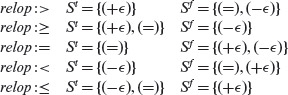
Let BR denote the following set of symbols {t, f, <, =, >, +ϵ, –ϵ}. Here “BR” is an abbreviation for “Boolean and Relational.” We shall refer to an element of the BR set as a BR-symbol.
A BR symbol specifies a constraint on a simple condition. For example, the symbol “f” can be used as a constraint for a < b. To satisfy this constraint, values of a and b must be chosen such that the condition is false.
A BR symbol specifies a constraint on a Boolean variable or a relational expression. For example, the symbol “+ϵ” is a constraint on the expression Ε′ : e1 < e2. Satisfaction of this constraint requires that a test case for Ε′ ensure that 0 < e1 – e2 ≤ ϵ. Similarly, the symbol “–ϵ” is another constraint on E′. This constraint can be satisfied by a test for Ε′ such that –ϵ ≤ e1 – e2 < 0.
A constraint C is considered infeasible for predicate pr if there exist no input values for the variables in pr that satisfy C. For example, constraint (>, >) for predicate a > b ∧ b > d requires the simple predicates a > b and d > a to be true. However, this constraint is infeasible if it is known that d > a.
A simple condition is constrained to a specific truth value by a predicate constraint. Thus, a compound condition has as many predicate constraints as there are simple condition in it.
Example 4.8 Consider the relational expression E : a < c + d. Now consider constraint “C : (=)” on E. While testing Ε for correctness, satisfying C requires at least one test case such that a = c + d. Thus the test case < a = 1, c = 0, d =1 >ϵ satisfies the constraint C on E.
As another example, consider the constraint C : (+ϵ) on expression Ε given above. Let ϵ = 1. A test to satisfy C requires that 0 < a – (c + d) ≤ 1. Thus, the test case < a = 4, c = 2, d = 1 > satisfies constraint (+ϵ) on expression E.
Similarly, given a Boolean expression Ε : b, the constraint “t” is satisfied by a test case that sets variable b to true.
BR symbols t and f are used to specify constraints on Boolean variables and expressions. A constraint on a relational expression is specified using any of the three symbols <, =, and >. Symbols t and f can also be used to specify constraints on a simple relational expression when the expression is treated as a representative of a Boolean variable. For example, expression pr : a < b could serve as a representative of a Boolean variable z in which case we can specify constraints on pr using t and f.
A predicate constraint for a condition is considered infeasible if it cannot be satisfied by any value of the variables in the condition.
We will now define constraints for entire predicates that contain Boolean variables and relational expressions joined by one or more Boolean operators.
Let pr denote a predicate with n, n > 0, ∧ and ∨ operators. A predicate constraint C for predicate pr is a sequence of (n + 1) BR symbols, one for each Boolean variable or relational expression in pr. When clear from context, we refer to “predicate constraint” as simply constraint.
A predicate constraint for a compound predicate having n simple conditions is a sequence of (n + l) BR symbols, one for each simple condition.
We say that a test case t satisfies C for predicate pr, if each component of pr satisfies the corresponding constraint in C when evaluated against t. Constraint C for predicate pr guides the development of a test for pr, i.e. it offers hints on the selection of values of the variables in pr.
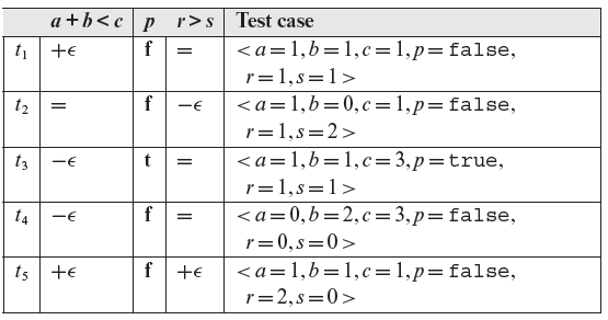
Example 4.9 Consider the predicate pr : b ∧ r < s ∨ u ≥ v. One possible BR-constraint for pr is C : (t, =, >). Note that C contains three constraints one for each of the three components of pr. Constraint t applies to b, = to r < s, and > to u ≥ v. The following test case satisfies C for pr.
<b = true, r = 1, s = 1, u = 1, v = 0>
Several other test cases also satisfy C for pr. The following test case does not satisfy C for pr.
<b = true, r = 1, s = 1, u = 1, v = 2>
as the last of the three elements in C is not satisfied for the corresponding component of pr which is u ≥ v.
Given a constraint C for predicate pr, any test case that satisfies C makes pr either true or false. Thus, we write pr(C) to indicate the value of pr obtained by evaluating it against any test case that satisfies C. A constraint C for which pr(C) = true is referred to as a true constraint and the one for which pr(C) evaluates to false is referred to as a false constraint. We partition a set of constraints S into two sets St and Sf such that S = St ∪ Sf . The partition is such that for each C ϵ St, pr(C) = true and for each C ϵ Sf , pr(C) = false.
A test case that satisfies a true constraint makes the corresponding predicate evaluate as true. Similarly, a test case that satisfies a false constraint makes the corresponding predicate evaluate as false.
Example 4.10 Consider the predicate pr : (a < b)∧(c > d) and constraint C1 : (=, >) on pr for ϵ = 1. Any test case that satisfies C1 on pr, makes pr evaluate to false. Hence C1 is a false constraint. Consider another constraint C2 : (<,+ϵ) for ϵ = 1 on predicate pr. Any test case that satisfies C2 on pr, makes pr evaluate to true. Hence C2 is a true constraint. Now, if S = {C1, C2} is a set of constraints on predicate pr, then we have St = {C2} and Sf = {C1}.
4.4.4 Predicate testing criteria
We are interested in generating a test set Τ from a given predicate pr such that (a) Τ is minimal and (b) Τ guarantees the detection of any fault in the implementation of pr that conforms to the fault model described earlier. Towards the goal of generating such a test set, we define three criteria commonly known as the BOR, BRO, and BRE testing criteria. The names BOR, BRO, and BRE correspond to, respectively, “Boolean Operator,” “Boolean and Relational Operator,” and “Boolean and Relational Expression.” Formal definitions of the three criteria follow.
A BOR adequate test set is guaranteed to detect all errors that correspond to our fault model. Tests that are BRO and BRE adequate are likely to detect errors that correspond to our fault model.
- A test set Τ that satisfies the BOR testing criterion for a compound predicate pr, guarantees the detection of single or multiple Boolean operator faults in the implementation of pr. Τ is referred to as a BOR-adequate test set and sometimes written as TBOR.
- A test set Τ that satisfies the BRO testing criterion for a compound predicate pr, is likely to detect single Boolean operator and relational operator faults in the implementation of pr. Τ is referred to as a BRO-adequate test set and sometimes written as TBRO.
- test set Τ that satisfies the BRE testing criterion for a compound predicate pr, is likely to detect single Boolean operator, relational expression, and arithmetic expression faults in the implementation of pr. Τ is referred to as a BRE-adequate test set and sometimes written as TBRE.
The term “guarantees the detection of” is to be interpreted carefully. Let Tx, x ϵ {BOR, BRO, BRE}, be a test set derived from predicate pr. Let pf be another predicate obtained from pr by injecting single or multiple faults of one of three kinds: Boolean operator fault, relational operator fault, and arithmetic expression fault. Tx is said to guarantee the detection of faults in pf if for some t ϵ Tx, p(t) ≠ pf(t). The next example shows a sample BOR-adequate test set and its fault detection effectiveness.
Example 4.11 Consider the compound predicate pr : a < b ∧ c > d. Let S denote a set of constraints on pr; S = {(t, t), (t, f), (f, t)}. The following test set Τ satisfies constraint set S and the BOR testing criterion.
As Τ satisfies the BOR testing criterion, it guarantees that all single and multiple Boolean operator faults in pr will be revealed. Let us check this by evaluating pr, and all its variants created by inserting Boolean operator faults, against Τ.
Table 4.2 Fault detection ability of a BOR-adequate test set Τ of Example 4.11 for single and multiple Boolean operator faults. Results of evaluation that distinguish the faulty predicate from the correct one are underlined.
Table 4.2 lists pr and a total of 7 faulty predicates obtained by inserting single and multiple Boolean operator faults in pr. Each predicate is evaluated against the three test cases in T. Note that each faulty predicate evaluates to a value different from that of pr for at least one test case.
It is easily verified that if any column is removed from Table 4.2, at least one of the faulty predicates will be left indistinguishable by the tests in the remaining two columns. For example, if we remove test t2 then the faulty predicate 6 cannot be distinguished from pr by tests t1 and t3. We have thus shown that Τ is minimal and BOR adequate for predicate pr.
Exercise 4.11 is similar to the one above and asks you to verify that the two given test sets are BRO and BRE adequate, respectively. In the next section we provide algorithms for generating BOR, BRO, and BRE adequate tests.
4.4.5 BOR, BRO, and BRE adequate tests
We are now ready to describe the algorithms that generate constraints to test a predicate. The actual test cases are generated using the constraints. Recall that a feasible constraint can be satisfied by one or more test cases. Thus, the algorithms we describe are to generate constraints and do not focus on the generation of the specific test cases. The test cases to satisfy the constraints can be generated manually or automatically. Let us begin by describing how to generate a BOR constraint set for a give predicate.
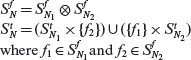
Consider the following two definitions of set products. The product of two finite sets A and B, denoted as Α × Β is defined as follows.
We need another set product in order to be able to generate minimal sets of constraints. The onto set product operator, written as ⊗, is defined as follows. For finite sets A and Β, A ⊗ Β is a minimal set of pairs (u, ν) such that u ϵ A, ν ϵ B, and each element of A appears at least once as u and each element of Β appears at least once as v. Note that there are several ways to compute A ⊗ Β when both A and Β contain two or more elements.
The cross product of two sets is unique. However, the onto product of two sets may not be unique.
Example 4.12 Let A = {t, =, >} and B = {f, <}. Using the definitions of set product and the onto product, we get the following sets:
Notice that there are six different ways to compute A ⊗ B. The algorithms described next select any one of the different sets.
Given a predicate pr, the generation of the BOR, BRO, and BRE constraint sets requires the abstract syntax tree for pr denoted as AST(pr). Recall that (a) each leaf node of AST(pr) represents a Boolean variable or a relational expression and (b) an internal node of AST(pr) is a Boolean operator such as ∧, ∨, , and ¬ known as an AND node, OR node, XOR node, and NOT node, respectively.
We now introduce four procedures for generating tests from a predicate. The first three procedures generate BOR, BRO, and BRE adequate tests for predicates that involve only singular expressions. The last procedure, named BOR-MI, generates tests for predicates that contain at least one non-singular expression. See Exercise 4.20 for an example that illustrates the problem in applying the first three procedures below to a non-singular expression.
The BOR constraint set
Let pr be a predicate and AST(pr) its abstract syntax tree. We use letters such as N, N1, and N2 to refer to various nodes in the AST(pr). SN denotes the constraint set attached to node N. As explained earlier, ![]() and
and ![]() denote, respectively, the true and false constraint sets associated with node N;
denote, respectively, the true and false constraint sets associated with node N; ![]() The following algorithm generates the BOR constraint set for pr.
The following algorithm generates the BOR constraint set for pr.
An abstract syntax tree (AST) captures the syntactic relationships among the constituent elements of a predicate. The well-known parsing technique, often used in compilers, can be used to construct an AST for any predicate.
Procedure for generating a minimal BOR constraint set from an abstract syntax tree of a predicate pr.
|
Input: |
An abstract syntax tree for predicate pr, denoted by AST(pr). pr, contains only singular expressions. |
|
Output : |
BOR constraint set for pr attached to the root node of AST(pr). |
Procedure: BOR-CSET
|
Step 1 |
Label each leaf node Ν of AST(pr) with its constraint set S(N) for each leaf SN = {t, f}. |
|
Step 2 |
Visit each non-leaf node in AST(pr) in a bottom up manner. Let N1 and N2 denote the direct descendants of node N, if N is an AND- or an OR-node. If N is a NOT-node, then N1 is its direct descendant. SN1 and SN2 are the BOR constraint sets for nodes N1 and N2, respectively. For each non-leaf node N, compute SN as follows |
|
2.1 |
N is an OR-node: |
|
|
|
|
2.2 |
N is an AND-node: |
|
|
|
|
2.3 |
N is NOT-node: |
|
|
|
|
Step 3 |
The constraint set for the root of AST(pr) is the desired BOR constraint set for pr. |
End of Procedure BRO-CSET
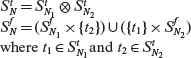
A BOR constraint set consists of n-tuples of BR symbols t and f, where n is the number of simple conditions in the predicate.
The BOR constraint set is generated by assigning constraints to the leaf nodes of an abstract syntax tree. Constraints at the leaves are then propagated up the tree using rules defined in the algorithm. The derived constraint set as available at the root node.
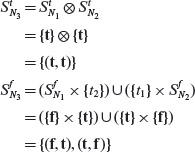
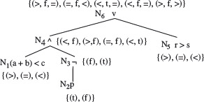
Example 4.13 Let us apply the procedure described above to generate the BOR-constraint sets for the predicate p1 : a < b ∧ c > d used in Example 4.11. The abstract syntax tree for p1 is shown in Figure 4.11(a).
Figure 4.11 BOR constraint sets for predicates (a) a < b ∧ c > d and (b) (a + b) < c ∧ ¬p ∨ (r > s). The constraint sets are listed next to each node. See the text for the separation of each constraint set into its true and false components.
N1 and N2 are the leaf nodes. The constraint sets for these two nodes are given below.
Traversing AST(p1) bottom up, we compute the constraint set for non-leaf N3 which is an AND-node.
Thus, we obtain SN3 = {(t, t), (f, t), (t, f} which is the BOR-constraint set for predicate p1. We have now shown how SN3, used in Example 4.11, is derived using a formal procedure.
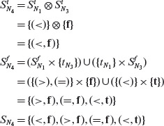
Example 4.14 Let us compute the BOR constraint set for predicate p2 : (a + b < c) ∧ ¬p ∨ (r > s) which is a bit more complex than predicate p1 from the previous example. Note that the ∧ operator takes priority over the ∨ operator. Hence p2 is equivalent to the expression ((a + b < c) ∧ (¬p)) ∨ (r > s).
An AST is traversed bottom-up to derive the BOR constraint set for a predicate. Given that the onto set product is used in the construction of the constraint set, the resulting set may not be unique.
First, as shown in Figure 4.11(b), we assign the default BOR constraint sets to the leaf nodes N1, N2, and N5. Next we traverse AST(p2) bottom up and breadth first. Applying the rule for a NOT node, we obtain the BOR constraint set for N3 as follows:
The following BOR constraint set is obtained by applying the rule for the AND-node.
Using the BOR constraint sets for nodes N4 and N5 and applying the rule for OR-node, we obtain the BOR constraint set for node N6 as follows:
Notice that we could select any one of the constraints (f, f) or (t, t) for fN4. Here we have arbitrarily selected (f, f). Sample tests for p2 that satisfy the four BOR constraints are given in Table 4.3. Exercise 4.13 asks you to confirm that indeed the test set in Table 4.3 is adequate with respect to the BOR testing criterion.
Table 4.3 Sample tests cases that satisfy the BOR constraints for predicate p2 derived in Example 4.14.
A test set for a predicate is derived from its BOR constraint set by selecting suitable values of the variables involved in the predicate.
The BRO constraint set
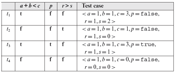
Recall that a test set adequate with respect to a BRO constraint set for predicate, pr, is very likely to detect all combinations of single or multiple Boolean operator and relational operator faults. The BRO constraint set S for a relational expression e1 relop e2 is {(>), (=), (<)}. As shown below, the separation of S into its true and false components depends on relop.
The BRO constraint set is useful when deriving tests for predicates that involve relational operators.
We now modify Procedure BOR-CSET introduced earlier for the generation of the minimal BOR constraint set to generate a minimal BRO constraint set. The modified procedure follows.
Procedure for generating a minimal BRO constraint set from an abstract syntax tree of a predicate pr.
|
Input: |
An abstract syntax tree for predicate pr, denoted by AST(pr). pr, contains only singular expressions. |
|
BRO constraint set for pr attached to the root node of AST(pr). |
Procedure: BRO-CSET
|
Step 1 |
Label each leaf node Ν of AST(pr) with its constraint set SN. For each leaf node that represents a Boolean variable, SN = {t, f}. For each leaf node that is a relational expression, SN = {(>), (=), (<)}. |
|
Step 2 |
Visit each non-leaf node in AST(pr) in a bottom up manner. Let N1 and N2 denote the direct descendants of node N, if N is an AND- or an OR-node. If N is a NOT-node, then N1 is its direct descendant. SN1 and SN2 are the BRO constraint sets for nodes N1 and N2, respectively. For each non-leaf node N, compute SN as per Steps 2.1, 2.2, and 2.3 in Procedure BRO-CSET. |
|
Step 3 |
The constraint set for the root of AST(pr) is the desired BRO constraint set for pr. |
End of Procedure BRO-CSET
The algorithm for deriving a BRO constraint set is similar to that for deriving a BOR constraint set. The primary difference is in the constraints assigned to the leaf nodes.
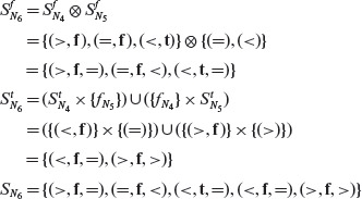
Example 4.15 Let us construct a BRO constraint set for predicate pr : (a + b) < c ∧ ¬p ∨ (r > s). Figure 4.12 shows the abstract syntax tree for pr with nodes labeled by the corresponding BRO constraint sets. Let us derive these sets using Procedure BRO-CSET.
First, the leaf nodes are labeled with the corresponding BRO constraint sets depending on their type. Next we traverse the tree bottom up and derive the BRO constraints for each node from those of its immediate descendants. The BRO constraint set for node N3, as shown in Figure 4.12, is derived using Step 2.3 of Procedure BOR-CSET.
Figure 4.12 BRO constraint set for predicate pr = (a + b) < c ∧ ¬p ∨ (r > s). The constraint sets are listed next to each node. See the text for the separation of each constraint set into its true and false components.
Next we construct the BRO constraint set for the AND node N4 using Step 2.2.
Finally we construct the BRO constraint set for the root node N6 by applying Step 2.1 to the BRO constraint sets of nodes N4 and N5.
Sample tests for pr that satisfy the five BRO constraints are given in Table 4.4. Exercise 4.14 asks you to confirm that indeed the test set in Table 4.4 is adequate with respect to the BRO testing criterion.
Table 4.4 Sample tests cases that satisfy the BRO constraints for predicate pr derived in Example 4.15.
The BRE constraint set
We now show how to generate BRE constraints that lead to test cases which are likely to detect any Boolean operator, relation operator, arithmetic expression, or a combination thereof, faults in a predicate. The BRE constraint set for a Boolean variable remains {t, f} as with the BOR and BRO constraint sets. The BRE constraint set for a relational expression is {(+ϵ), (=), (–ϵ)}, ϵ > 0. The BRE constraint set S for a relational expression e1 relop e2 is separated into subsets St and Sf based on the following relations.
A BRE constraint set is useful when deriving tests for relational expressions that contain arithmetic operator and are to be tested for errors such as “off by 1”.
Constraint |
Satisfying condition |
|---|---|
+ϵ |
0 < e1 − e2 ≤ +ϵ |
–ϵ |
–ϵ ≤ e1 − e2 < 0 |
Based on the conditions listed above, constraint S into its true and false components as follows:
The procedure to generate a minimal BRE-constraint set is similar to Procedure BRO-CSET. The key difference in the two procedures lies in the construction of the constraint sets for the leaves. Procedure BRE-CSET follows.
Procedure for generating a minimal BRE constraint set from an abstract syntax tree of a predicate pr.
|
Input: |
An abstract syntax tree for predicate pr, denoted by AST(pr). pr contains only singular expressions. |
|
|
|
Output: |
BRE constraint set for pr attached to the root node of AST(pr). |
|
Step 1 |
Label each leaf node Ν of AST(pr) with its constraint set SN. For each leaf node that represents a Boolean variable, SN = {t, f}. For each leaf node that is a relational expression, SN = {(+ϵ), (=), (–ϵ)}. |
|
Step 2 |
Visit each non-leaf node in AST(pr) in a bottom up manner. Let N1 and N2 denote the direct descendants of node N, if Ν is an AND- or an OR-node. If Ν is a NOT-node, then N1 is its direct descendant. SN1 and SN2 are the BRE constraint sets for nodes N1 and N2, respectively. For each non-leaf node N, compute SN as in Steps 2.1, 2.2, and 2.3 in Procedure BOR-CSET. |
|
Step 3 |
The constraint set for the root of AST(pr) is the desired BRE constraint set for pr. |
End of Procedure BRE-CSET
Example 4.16 Consider the predicate p : (a + b) < c ∧ ¬p ∨ r > s. The BRE constraint set for pr is derived in Figure 4.13. Notice the similarity of BRE and BRO constraints listed against the corresponding nodes in Figures 4.12 and 4.13.
Note that tests t1 through t4 in Table 4.5 are identical to the corresponding tests in Table 4.4. However, t5 in Table 4.4 does not satisfy the (+ϵ) constraint. Hence, we have a different t5 in Table 4.5. Exercise 4.17 asks you to compare the test cases derived from constraints using BRO-CSET and BRE-CSET.
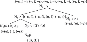
Figure 4.13 BRE constraint set for predicate (a + b) < c ∧ ¬p ∨ (r > s).
Table 4.5 Sample tests cases that satisfy the BRE constraints for predicate pr derived in Example 4.16 ϵ = 1.
4.4.6 BOR constraints for non-singular expressions
As mentioned earlier, the test generation procedures described in the previous sections generate BOR, BRO, and BRE adequate tests for predicates that do not contain any non-singular expressions. However, the presence of non-singular expressions might create conflicts while merging constraints during the traversal of the abstract syntax tree (see Exercise 4.20). Resolution of such conflicts leads to a constraint set that is not guaranteed to detect all Boolean operator faults that might arise in the implementation of the predicate under test. In this section, we generalize the BOR-CSET procedure to handle predicates that might contain non-singular expressions.
While constraint sets for non-singular predicates can be constructed directly by applying the procedures given earlier, more effective procedures are available.
A non-singular expression contains multiple occurrences of one or more literals. The BOR-CSET algorithm needs to be modified to generate constraints for such an expression.
Recall from Section 2.1 that a non-singular expression is one that contains multiple occurrences of a Boolean variable. For example, we list below a few non-singular expressions and their disjunctive normal forms; note that we have omitted the AND operator, used + to indicate the OR operator, and the over bar symbol to indicate the complement of a literal.
Predicate (pr) |
DNF |
Mutually singular components of pr |
|---|---|---|
ab(b + c) |
abb + abc |
a; b(b + c) |
a(bc + bd) |
abc + abd |
a; (bc + bd) |
a(bc + |
abc + a |
a; bc + |
There are standard algorithms for converting expressions from DNF to CNF form and vise-versa. These algorithms are not described in this book.
The modified BOR strategy to generate tests from predicate pr uses the BOR-CSET procedure and another procedure which we refer to as the Meaning Impact, or simply MI, procedure. Before we illustrate the BOR-MI strategy, we introduce the MI procedure for generating tests from any Boolean expression pr, singular or non-singular. The predicate pr must be in its minimal disjunctive normal form. If pr is not in DNF, then it needs to be transformed into one prior to the application of the MI-CSET procedure described next; there are standard algorithms for transforming any Boolean expression into an equivalent minimal DNF.
Procedure for generating a minimal constraint set from a predicate possibly containing non-singular expressions.
|
Input: |
A Boolean expression Ε = e1 + e2 + ..... en in minimal disjunctive normal form containing n terms. Term ei, 1 ≤ i ≤ n contains li > 0 literals. |
|
|
|
Output: |
A set of constraints SE that guarantees the detection of missing or extra NOT operator fault in a faulty version of E. |
Procedure: MI-CSET
|
Step 1 |
For each term ei, 1 ≤ i ≤ n, construct Tei as the set of constraints that make ei true. |
|
Step 2 |
Let |
|
Step 3 |
Construct |
|
Step 4 |
Let |
|
Step 5 |
Let |
|
Step 6 |
Construct |
|
Step 7 |
Construct the desired constraint set for E as |
End of Procedure MI-CSET
A logical expression, i.e. a predicate, is in disjunctive normal form when its constituents are combined using the OR logical operator. For example, if x, y, and z denote simple conditions, then (x OR y or z) is in disjunctive normal form and can also be written as (x + y + z).
The MI-CSET procedure generates a minimal constraint set for a predicate expressed in minimal disjunctive form. Tests generated from such constraint set guarantee the detection of missing or extra negation (NOT) operator.
Example 4.17 Let
where a, b, c, and d are Boolean variables. Note that Ε is non-singular as variable b occurs twice. The DNF equivalent of Ε is e1 + e2, where e1 = abc and
We now apply Procedure MI-CSET to generate sets
First, let us construct Te1 and Te2.
Next we construct TSe1 and TSe2.
Notice that as Te1 and Te2 are disjoint, we get TSe1 = Te1 and TSe2 = Te2. Selecting one test each from TSe1 and TSe2, we obtain a minimal set of constraints that make Ε true and cover each term of Ε as follows:
Note that there exist four possible
Next we construct constraints
, 1 ≤ i ≤ 2, 1 ≤ j ≤ 3. We have three terms corresponding to e1, namely
and
Similarly, we get three terms for e2, namely,
Next we remove from the above six sets any test cases that belong to any of the sets Tek,1 ≤ k ≤ n sets.
The test set that makes Ε false is now constructed by selecting tests from the six sets listed above such that
is minimal and covers each FS.
The set of constraints SE generated by the MI-CSET procedure for expression Ε contains a total of six constraints as follows:
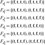
We are now ready to introduce the BOR-MI-CSET procedure for generating a minimal constraint set from a possibly non-singular expression. The procedure described next uses the BOR-CSET and the MI-CSET procedures described earlier.
Procedure for generating a minimal constraint set for a predicate possibly containing non-singular expressions.
|
Input: |
A Boolean expression E. |
|
Output: |
A set of constraints SE that guarantees the detection of Boolean operator faults in E. |
Procedure: BOR-MI-CSET
|
Step 1 |
Partition Ε into a set of n mutually singular components E ={E1,E2, . . . En}. |
|
Step 2 |
Generate the BOR constraint set for each singular component in Ε using the BOR-CSET procedure. |
|
Step 3 |
Generate the MI-constraint set for each non-singular component in Ε using the BOR-CSET procedure. |
|
Step 4 |
Combine the constraints generated in the previous two steps using Step 2 from the BOR-CSET procedure to obtain the constraint set for E. |
End of Procedure BOR-MI-CSET
The BOR-MI-CST procedure generates constraint set for a possibly non-singular logical expression. Tests generated from such a constraint set guarantee the detection of Boolean operator faults.
The following example illustrates the BOR-MI-CSET procedure.
Example 4.18 As in Example 4.17, let
, where a, b, c, and d are Boolean variables. Note that Ε is non-singular as variable b occurs twice. We follow the BOR-MI-CSET procedure to generate the constraint set SE.
From Step 1, partition Ε into components e1 and e2 , where e1 = a is a singular expression and
is a non-singular expression. In accordance with Step 2, use the BOR-CSET procedure to find Se1 as follows:
Next apply the MI-CSET procedure to generate the MI constraints for e2. Note that e2 is a DNF expression and can be written as e2 = u + ν where u = bc and
Applying Step 1 we obtain the following:
Applying Step 2 from the MI-CSET procedure to Tu and Tν, and then Step 3, we obtain the following sets:
Notice that there are several alternatives for
from which we need to select one. Next, derive the false constraint set
by applying Steps 4, 5, and 6. The complemented subexpressions needed in these steps are
v1 = bd, and
Here is a summary of what we have derived so far by applying Steps 1, 2, and 3 from procedure BOR-MI-CSET.
Now apply Step 4 to the constraints sets generated for subexpressions e1 an e2 and obtain the BOR constraint set for the entire expression E. This process is illustrated in Figure 4.14. The sets

and SE are listed below.
Figure 4.14 Constraint set for predicate
derived using the BOR-MI-CSET procedure.
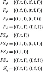
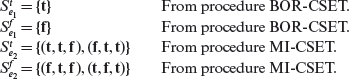
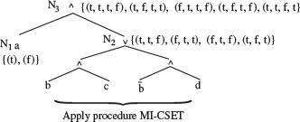
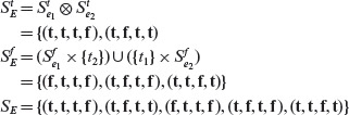
Notice that constraint set SE derived using the BOR-MI-CSET procedure contains only five constraints as compared to the six constraints in SE derived using the MI-CSET procedure in Example 4.17. It is generally the case that the constraint sets derived using the BOR-MI-CSET procedure are smaller, and more effective in detecting faults, than those derived using the MI-CSET procedure. Exercises 4.23 and 4.24 should help you sharpen your understanding of the BOR-MI-CSET procedure and the effectiveness of the tests generated.
4.4.7 Cause-effect graphs and predicate testing
Cause-effect graphing, as described in Section 4.3 is a requirements modeling and test generation technique. Cause-effect relations are extracted from the requirements. Each “cause” portion of a cause-effect relation can be expressed as a predicate. The “effect” portion is used to construct the oracle which decides if the effect does occur when the corresponding cause exists.
To test if the condition representing the cause in a cause-effect graph has been implemented correctly, one could generate tests using either the decision table technique described in Section 4.3.3 or one of the four procedures described in this section.
Empirical studies have revealed that the BOR-CSET procedure generates smaller test sets than the cause-effect graphing technique. However, note that the BOR method only considers predicates and not their effects.
Several studies have revealed that the BOR-CSET procedure generates significantly smaller tests sets than the CEGDT procedure described in Section 4.3.3. The fault detection effectiveness of the tests generated using the BOR-CSET procedure is only slightly less than that of tests generated using the CEGDT procedure.
The combination of cause-effect graphs and predicate testing procedures described in this section is considered useful for two reasons. First, the cause-effect graphs are a useful tool for modeling requirements. Second, once the graphical model has been built, any one of the four predicate-based test generation procedures introduced in this section can be applied for test generation. Exercise 4.25 is to help you understand how the combination of cause-effect graphs and predicate testing works.
4.4.8 Fault propagation
We now explain the notion of fault propagation that forms the basis of the four predicate test generation algorithms described in this section. Let pr be a predicate, simple or compound, and pc a component of pr. Each node in the abstract syntax tree of a predicate is a component of that predicate. For example, as in Figure 4.13, predicate p : (a + b) < c ∧ ¬p ∨ r > s contains the following six components: a + b < c, ∧, ¬, p, ∨, and r > s.
A test for an incorrect predicate p is considered error revealing if the evaluation of p against t leads to a value different from that obtained by evaluating the correct version of p against t.
Let pf be a faulty version of pr. We say that a fault in any component of pf propagates to the root node of AST(pf), i.e. effects the outcome of pf, if p(t) ≠ pf(t) for some test case t. Test t is also known as an error revealing or fault revealing test for pf.
In predicate testing we are interested in generating at least one test case t that ensures the propagation of the fault in pf. The BOR, BRO, and BRE adequate test sets are very likely to guarantee certain kinds of faults, mentioned in earlier sections, propagate to the root node of the predicate under test. The next example illustrates the notion of fault propagation.
Example 4.19 Let p : (a + b) < c ∧ ¬p ∨ r > s and pf : (a + b) < c ∨ ¬p ∨ r > s be two predicates where pf is a faulty version of pr. pf has a Boolean operator fault created by the incorrect use of the ∨ operator. Table 4.3 lists four test cases that form a BOR-adequate test set.
Figure 4.15 Abstract syntax trees in (a) and (b) show the failure of test t1 to force the propagation of the ∧ operator fault. (c) and (d) show how test t4 ensures the propagation of the ∧ operator fault.
Figure 4.15 (a) and (b) show that test t1 in Table 4.3 fails to cause the ∧ operator fault to propagate to the root node of AST(pf) and thus we have p(t1) = pf(t1). However, as shown in Figure 4.15 (c) and (d), test t4 does cause the fault to propagate to the root node of AST(pf) and thus we have p(t4) ≠ pf(t4).
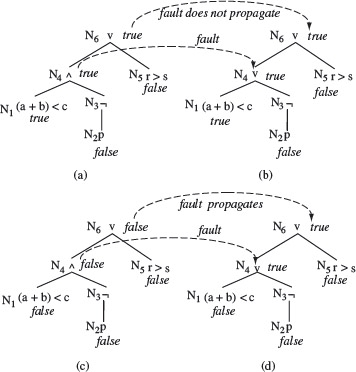
Given a predicate pr containing n AND/OR operators and Boolean variables, one can use a brute force method to generate a test set T with 2n tests. For example, predicate p : (a + b) < c ∧ ¬p ∨ r > s contains two Boolean AND/OR operators and one Boolean variable; thus n = 3. A test set Τ generated in a brute force manner will contain a total of eight tests cases that satisfy the following set S of eight constraints.
BOR, BRO, and BRE adequate test sets are generally smaller than those derived by enumerating all combinations of the truth values of the components of a compound predicate.
These eight constraints ensure that each relational expression and Boolean variable in pr will evaluate to true and false against at least one test case in Τ. Thus, Τ is obviously BOR, BRO, and BRE adequate. However, Τ is not minimal. Notice that while Τ contains eight test cases, a BRE adequate test set derived in Example 4.16 contains only five test cases.
A BOR, BRO, or BRE adequate test set contains 2*n +3 tests, where n is the number of AND or OR operators.
It can be shown that if a predicate pr contains n AND/OR operators, then the maximum size of the BOR adequate test set is n + 2. The maximum size of a BRO or BRE adequate test set for pr is 2 * n + 3 (see Exercise 4.18).
As indicated above, the size of BOR, BRO, and BRE adequate tests grows linearly in the number of AND/OR and Boolean variables in a predicate. It is this nice property of the test generation procedures introduced in this section, in addition to fault detection effectiveness, that distinguishes them from the brute force method and the cause-effect graph-based test generation introduced earlier in Section 4.3.
The linearity property mentioned above is the result of (a) using the abstract syntax tree of a predicate to propagate the constraints from leaves to the root node and (b) using the onto (⊗) product of two sets, instead of the set product (×), while propagating the constraints up through the abstract syntax tree (see Exercise 4.19).
4.4.9 Predicate testing in practice
Predicate testing is used to derive test cases both from the requirements and from the application under test. Thus it can be used for generating specification-based and program-based tests.
Specification-based predicate test generation
An analysis of application requirements reveals conditions under which the application must behave in specific ways. Thus, an analysis of application requirements might yield the following list of n conditions and the associated tasks.
Condition |
Task |
|---|---|
C1 |
Task1 |
C2 |
Task2 |
. . . |
|
Cn |
Taskn |
Such a list can be used to generate a test set Τ for the application under test. Note that each condition is represented by a predicate. The condition-task pairs in the list above are assumed independent in the sense that each task depends exclusively on the condition associated with it. The independence assumption does not hold when, for example, a condition, say C2, depends on C1 in the sense that C2 cannot be true if C1 is true. For example, two such dependent conditions are: C1 : a < b and C2 : a > b. Obviously, if Task1 and Task2 are associated exclusively with conditions C1 and C2, respectively, then only one of them can be performed for a given input.
As conditions can be compound and tasks can be conjoined, the independence requirement does not exclude the specification of two tasks to be performed when a condition is true, or that one task requires two conditions to hold. Two tasks could be conjoined to form one tasks corresponding to a condition. Similarly, two conditions could be combined to form a single condition associated with a single task.
For test generation, one first selects an appropriate test generation algorithm described in this section. Different algorithms could be used for different conditions. For example, if condition C2 is represented by a non-singular predicate, then the BOR-MI-CSET algorithm will likely be preferred.
Once the test generation procedure is selected for a predicate, one generates a distinct test set. The union of the test sets so generated is a consolidated test set Τ for the application. It is certainly possible that two conditions yield the same test set.
Testing the application against test cases in Τ guarantees the detection of certain faults, indicated in Section 4.4.1, due to the incorrect coding of conditions from which the tests are derived. However, such a guarantee is valid only under certain conditions. The next example illustrates why a test set might fail.
Example 4.20 Suppose that we are to test system X. Requirements for X indicate that task Task1 is to be performed when condition C1 : a < b ∧ c > d is true. Tests for C1 are derived in Example 4.13 and are guaranteed to detect any Boolean operator fault in C1.
Now consider an implementation of X whose structure is abstracted in Figure 4.16. Statement S1 contains a fault in the coding of C1· The condition coded is Cf : a < b ∨ c > d. Let us assume that S1 is unreachable for any test input.
Figure 4.16 An implementation to illustrate why a predicate test that is theoretically guaranteed to detect any Boolean operator fault, might fail to do so in practice.
Suppose that statement S2 has been added by mistake, it should not be in the program. The condition C in S2 is C ∧ u, where u is a Boolean variable input to X. Now suppose that u is set to true while testing X to check for the correct execution of Task1.
The first three rows in the table below show that the observed behavior of X for each of the tests derived using the BOR-CSET procedure for condition C is identical to the expected behavior. However, when X is tested with u = false and the BOR constraint (t, t), the error is revealed.
A test set that theoretically is guaranteed to detect an error in a predicate might fail to do so in practice. This could happen, for example, due to an infeasible path.
Thus we have shown an instance where a test generated using the BOR-CSET procedure is unable to reveal the error. Certainly, this example is not demonstrating any weakness in the error detection effectiveness of the BOR-CSET procedure. Instead, it demonstrates that some errors in the program might mask an error in the implementation of a predicate.
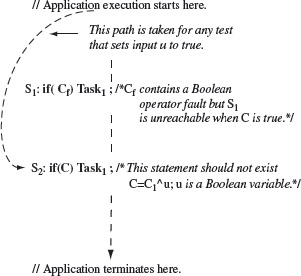
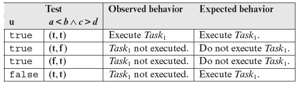
Program-based predicate test generation
Test sets can also be derived from predicates in the program. Test sets so derived are often referred to as white box tests. When executing such tests, one needs to ensure that the flow of control reaches the region in the program that implements the predicate being tested. As illustrated in the next example, this might cause some difficulty as several other conditions may need to be satisfied for the control to reach the desired region in the program.
Tests can be derived for predicates obtained from the requirements or from the code.
Example 4.21 Consider the following program that uses two conditions to control the execution of three tasks named task1, task2, and task3. Using inputs r and e, the program determines values of parameters a, b, c, and d.
Program P4.1
1 begin
2 int a, b, c, d, r, e;
3 input (r, e) ;
4 getParam (r, e);
5 if (e < 0)
6 then
7 task1 (a, b) ;
8 else
9 if (a < b&& c > d)
10 then
11 task2 (c, d) ;
12 else
13 task3 (c, d) ;
14 end
Suppose that the BOR-CSET procedure has been used to generate BOR-constraints from the predicate a < b && c > d. Satisfying these constraints would be relatively easier if the parameters a, b, c, and d were program inputs. However, as is the case in our example program, these four parameters depend on the values of r and e. Thus, satisfying these constraints will require a determination of the relationship between r, e, and the four parameters.
Further, one must ensure that all tests of P4.1 that correspond to the constraints force the program to reach the statement containing the predicate, i.e. line 9. While this seems easy for our example program, it might not be so in most real-life programs.
4.5 Tests Using Basis Paths
Recall from Chapter 2 that a basis set is a set of basis paths derived from the CFG of a program. The basis paths are linearly independent complete paths. The following procedure can be used for generating tests for program Ρ using basis paths.
Given a program P, one can find a set of basis paths that are linearly independent. All other paths in P can be derived as a linear combination of the basis paths. A path condition associated with a basis path serves as a source of tests.
- Generate the CFG G from P.
- Generate the basis set from G.
- Do the following for each path in the basis set:
- Find the path condition expressed in terms of the input variables.
- Select values of the input variables that make the path condition true.
- Determine the expected output for the input values selected above.
The above procedure will generate at least as many tests as there are basis paths. The next example illustrates the above process.
Example 4.22 Figure 4.17 shows the CFG of Program P3.1. The cyclomatic complexity of the CFG is 11 – 9 + 2 = 4. The following four basis paths are derived from this CFG.
Figure 4.17 CFG for Program P4.1. Numbers against each node in the CFG correspond to the lines of code that belong to the corresponding basic block. (t) indicates the portion of the code executed when the condition at the indicated line is true, t and f label, respectively, the true and false branches.
p1 (Start, 1, 2, End)
p2 (Start, 1, 3, 4, End)
p3 (Start, 1, 3, 5, 6, End)
p4 (Start, 1, 3, 5, 7, End)
The table below lists the path conditions, inputs that satisfy the conditions and expected response of the program. A “Don’t care” entry indicates that the value could be arbitrary. File names “Exists”, “DoesNotExist”, and “Empty” indicate, respectively, a file that exists, does not exist, and is empty. For p4 it is assumed that the given word appears four times in the input file.
Execution of the above tests requires the existence of two files, one that exists but is empty, and the other that exists and contains at least one occurrence of the given word. Processing of the exception raised by the first of the four tests above might lead to additional response items that are not shown above.
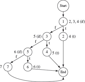
4.6 Scenarios and Tests
During system testing one often generates user-defined scenarios as tests. The assumption here is that a potential use of the system has an idea of how she wishes to use the system and hence can generate a few usage scenarios. Of course, a user in this case can also be the system tester.
A scenario is a story that describes the behavior of a system under certain constraints. User related scenarios derived from system requirements can be used to generate tests. Such kind of testing is useful when a complete system, or an application, is tested.
A scenario describes a likely use of the systems features. It is a partial behavioral description of the system under test. Thus, one scenario is likely to test several features of a system. A scenario is generated based on the system requirements. It is assumed that the user of the tester generating scenarios knows what the requirements are.
A scenario may consist of events such as “ignition key is inserted,” “ignition is turned ON,” “gear is changed from neutral to first,” and so on. In some cases a scenario might also consist of a sequence of activities where each activity is a sequence of events. Thus, a scenario becomes a kind of story line consisting of one or more events. The events could be natural, for example, earthquake, mechanical, for example, ignition turned ON, business, for example, order placed, or of any other kind.
An event-based scenario would be useful in testing a variety of devices, small or large such as a mobile phone or an automobile dashboard control software as well as business software, such as inventory management or finance management. A scenario is also useful in testing specific properties of a system. For example, a test scenario might be designed to check if the system can withstand a kind of attack such as denial of service or identity spoofing, or to test the performance of a system under certain conditions.
For a scenario to serve as a test case, each event in the scenario must be described explicitly. An event could be a user action or an input from another application in its environment.
For a scenario to be used as a test case, each event in the scenario must correspond to an observable response from the system under test. This leads to a scenario being a sequence of event-response pairs. Each event in the pair is input to the system manually or automatically. In the latter case some kind of a scenario simulator is needed that will create and apply the events, observe and analyze the system response to the event, and log it for future analysis.
Example 4.23 iDatify is a web-based tool for asking structured questions. Once created, a question can be made available to all users of the internet or to a specific community of people. Thus, two significant use-cases of iDatify are: question creation and community creation. Once a community has been created, questions can be created and associated with this community.
Event/Activity
Response
Start iDatify
Login window visible.
Login
Home page for the user visible.
Select “Create community”
“New Community” form visible
Fill the form, select “Create”
Confirmation message displayed
Select “Ask a question”
“New Question” page visible
Add a question with response fields.
Create question visible
Select “Submit”
Question submitted confirmation message displayed.
Select “My communities”
Community just created is displayed.
Select “Ask a New Question”
“New Question” page visible
Add another question with response fields.
Create question visible
Select “Submit”
Question submitted confirmation message displayed.
Select “My communities”
Community just created is displayed.
Select the community just created
Community displayed. Both questions should be visible.
Below is a scenario to test the question and community creation features of iDatify. The scenario below is described in terms of user actions (events) and iDatify responses and may not be valid for any version of iDatify other than Version 0.23.
The underlined keywords above indicate an event or an activity. Notice that some activities, for example creating a question, are repeated. Repetition of events or activities within a scenario is intended to expose errors of initialization of variables.
Testing of complex system may require a large number of scenarios. Some of these scenarios ought to be aimed at testing the robustness of the system under test.
Testing of most complex systems will likely require hundreds or thousands of test scenarios. Manual execution of the test scenarios might be practically impossible as well as error prone. Thus, it is almost necessary to automate the process of scenario-based testing. For such systems, even the generation of scenarios is best done automatically from formal specifications such as finite state machines, UML diagrams, statecharts, and Z.
SUMMARY
In this chapter we have introduced another class of foundational techniques for generating tests. As in the previous chapter, the techniques in this chapter also partition the input domain, the focus is primarily the analysis of predicates to generate tests. A fault model for predicate testing is introduced. The BOR, BRO, and BRE techniques fall under the general category of syntax-based test generation. While these three techniques aim to detect the same types of errors as detected by the techniques mentioned above, the method used for test generation makes explicit use of the predicate syntax to generate tests and hence is quite different from the others.
Exercises
4.1 Consider the following variant of the program in Example 4.1.
1 String f(int x, int y){
2 int q=0, z=0; String s= ‘‘ ’’;
3 if(y<x+1) // Error 1: this should be y<x+2
4 {s=s+‘‘1’’; q=y*2;}
5 if(q-x>0)
7 if(z<=0) // Error 2: this should be z<0
8 s=s+‘‘3’’;
9 s=s+‘‘4’’;
10 return s;
11 }
Develop path condition for a path that goes through all three if statements. Generate tests as ON and OFF points for the path domain. Execute f against all tests and determine whether or not the errors are detected.
4.2 Consider the following incorrect function that contains a nonlinear path-condition.
1 int f(double x, double y){
2 if(x*x<y) // Correct condition is x*x < y*y
3 return 1;
4 else
5 return 2;
6 }
Using the domain testing method develop test cases for the above function. Under what conditions will the generated tests detect the error?
4.3 An internet-enabled automatic Dog Food Dispenser, referred to as iDFD, consists of two separate dispensers: a food dispenser (FD) and a water dispenser (WD). Each dispenser is controlled by a separate timer which has a default setting of 8 hours and can also be set to a different period. Upon a timer interrupt the iDFD dispenses water or food depending on whether it is a water-timer or a food-timer interrupt. A fixed amount of food or water is dispensed.
The iDFD has two sets of three identical indicators, one for the food and the other for water. The indicators are labeled “Okay”, “Low”, and “Empty.” After each dispensation, the iDFD checks the food and water levels and updates the indicators.
The iDFD can be connected to the internet via a secure connection. It allows an authorized user to set or reset the timers and also determine the water and food level in the respective containers. An email message is sent to the authorized dog sitter when food or water dispensation results in the corresponding indicators to show “Low” or “Empty.”
The iDFD is controlled by an embedded microprocessor, and the iDFD control software, that is responsible for the correct operation of all the functions mentioned above. You are required to generate test inputs to test the control software in the following three steps:
- Identify all causes and effects.
- Relate the causes and effects through a cause-effect graph.
- Create a decision table from the cause-effect graph you have generated.
- Generate test inputs from the decision table.
While executing the steps above, you may need to resolve any ambiguities in the requirements. Also, consider separating the test inputs from water and food dispensers.
4.4 In Example 4.5 we ignored the effects of buyer selections on the GUI updates. For example, when a user selects CPU 3, the monitor window contents change from displaying all three monitors to displaying only monitor Μ 30. (a) Identify all such GUI related effects in the GUI-based computer purchase system in Example 4.5. (b) Draw a cause-effect graph that relates the causes given in the example to the effects you have identified. (c) Transform your cause-effect graph to a decision table, (d) Generate test data from the decision table.
4.5 Consider the four cause-effect graphs in Figure 4.18. (a) For each graph in the figure, generate combinations of input conditions (causes) that bring Ef to 1-state. Do not apply the heuristics given in Section 4.3.4. (b) Now reduce the combinations generated in (a) by applying the heuristics. How much reduction, measured in terms of the number of combinations discarded, do you achieve in each case ? (c) Are the combinations generated in (b) unique in the sense that another set of combinations would also be satisfactory and as small in number ?
Figure 4.18 Cause-effect graphs for Exercise 4.5.
4.6 Construct a sample implementation I to show that the application of heuristic H2 from Table 4.1 will leave out at least one test that would have detected the error in I.
4.7 Consider the following modified versions of heuristics H1 and H4 given in Table 4.1.
H1: Enumerate any one combination of inputs to n1 and n2 such that n1= n2 = 0.
H4: Enumerate all combinations of inputs to n1 and n2 such that n1 = n2 = 1.
Discuss why the above modifications are undesirable (or desirable).
4.8 Complete Example 4.5 by (a) creating a decision table using procedure CEGDT; apply heuristics from Table 4.1 while generating the decision table. (b) Generate a set of tests from the decision table.
4.9 Complete Example 4.6 by reducing the combinations in the decision table using heuristics given in Table 4.1. Generate a set of tests given the following causes.
C1: A user selects Save As.
C2: A user selects Open.
C3: A user types in an integer greater than 99 in the relevant window.
C4: A user selects any one of the following values from a list: High or Medium.
4.10 Consider the following relational expression Ec: 2 * r < s + t, where r, s, and t are floating point variables. Construct three faulty versions of Ec that contain, respectively, the off-by-ϵ, off-by-ϵ*, and off-by-ϵ+ faults. Select a suitable value for ϵ.
4.11 Consider the condition C : (a + 1 > b)∧ (C = d), where a, b, c, and d are type compatible variables. (a) Let S1 = {(>, =), (>, >), (>, <), (=, =),(<, =)} be a set of constraints on C. As in Example 4.11, construct a test set T1 that satisfies S1 and show that T is BRO-adequate. (b) Now consider the constraint set S2 = {(+ϵ, =), (=, –ϵ), (–ϵ, =), (+ϵ, +ϵ)} on C. Construct a test set T2 that satisfies S2. Is T BRE adequate ? Assume that ϵ = 1.
4.12 Let A = {(<, =), (>, <)} and Β = {(t, =), (t, >), (f, <)} be two constraint sets. Compute A × B and A ⊗ B.
4.13 Consider the predicate p2 : (a + b) < c ∧ ¬p ∨(r > s) in Example 4.14. Confirm that any predicate obtained by inserting a Boolean operator fault in p2 will evaluate to a value different from that of p2 on at least one of the five test cases derived in Example 4.14.
4.14 Consider the predicate pr : (a + b) < c ∧ ¬p ∨ (r > s) in Example 4.15. Confirm that any predicate obtained by inserting single or multiple Boolean operator and relational operator faults in pr will evaluate to a value different from that of pr on at least one of the four test cases derived in Example 4.15.
4.15 For predicate pr, the BRO adequate test set TBRO in Table 4.4 contains one more test case than the BOR adequate test set TBRO in Table 4.3. (a) Is there a faulty predicate obtained from pr that will be distinguished from pr by TBRO and not by TBOR ? (b) Is there a faulty predicate obtained from pr that will be distinguished from pr by TBOR and not by TBRO ? Constrain your answer to the fault model in Section 4.4.1.
4.16 Consider a predicate pr and test sets TBRO and TBRE that are, respectively, BRO and BRE-adequate for pr. For what value of ϵ are TBRO and TBRE equivalent in their fault detection abilities ?
4.17 (a) Show that a BRE constraint set can derived from a BRO constraint set simply by replacing constraint (>) by (+ϵ), (<) by (–ϵ) and retaining (=). (b) Explain why a BRO-adequate test set might not be BRE-adequate. (c) Is a BRE-adequate test set always BRO-adequate ? BOR-adequate ? (d) Is a BRO-adequate test set always BOR-adequate ?
4.18 Let pr be a predicate that contains at most n AND/OR operators. Show that |TBOR| ≤ n + 2, |TBRO| ≤ 2 * n + 3, and |TBRE| ≤ 2 * n + 3.
4.19 Procedures BOR-CSET, BRO-CSET, and BRE-CSET use the ⊗ operator while propagating the constraints up through the abstract syntax tree. Show that larger test sets would be generated if instead the × operator is used.
4.20 What confdict(s) might arise when applying any of procedures BOR-CSET, BRO-CSET, and BRE-CSET to a predicate containing one or more non-singular expressions ? Answer this question using predicate pr : (a + b)(bc) and applying any of the three procedures.
4.21 Use the BOR-CSET procedure to generate tests from the predicate pr : a + b. (a) Do the tests generated guarantee the detection of the missing Boolean variable fault that causes the implementation of pr to be a ? (b) Do the tests generated guarantee the detection of the extra Boolean variable fault in coding pr that causes the implementation to be a + b + c, where c is the extra Boolean variable ?
4.22 In procedure MI-CSET in Section 4.4.6, show that (a) ![]() for 1 ≤ i ≤ n and (b)
for 1 ≤ i ≤ n and (b) ![]() for different terms in pr may not be disjoint and may be empty.
for different terms in pr may not be disjoint and may be empty.
4.23 Use the constraint set SE derived in Example 4.18 to show that the following faulty versions of the predicate ![]() evaluate differently than Ε on at least one test case derived from SE.
evaluate differently than Ε on at least one test case derived from SE.
4.24 (a) Use the BOR-MI-CSET procedure to derive the constraint set for the following predicate pr.
(a < b)∧ (((r > s) ∧ u) ∨ (a ≥ b) ∨ ((c < d) ∨ (f = g)) ∧ (v ∧ w)),
where a, b, c, d, f, g, r, and s are integer variables and u, v, and w are Boolean variables.
(b) Using the constraint set derived in (a), construct a test set Τ for pr. (c) Verify that Τ is able to distinguish the following faulty versions from pr.
- (a < b) ∧ ((¬(r > s)∧ u) ∨ (a ≥ b) ∨ ((c < d) ∨ (f = g)) ∧ (v ∧ w)); Incorrect NOT operator.
- (a < b) ∧ (((r > s) ∧ u) ∨ (a ≥ b)∨((c < d) ∨ (f = g))∧(
 ∧ w); Incorrect NOT operator.
 - (a < b) ∨ (((r > s) ∨ u) ∨ (a ≥ b) ∨ ((c < d) ∨ (f = g)) ∧ (v ∧ w)); Two incorrect OR operator.
- (a < b) ∨ (((r > s) ∧ ū) ∨ (a ≥ b) ∨ ((c < d) ∨ (f = g)) ∧ (v ∧ w)); Incorrect OR and NOT operators.
4.25 Consider the cause-effect graph shown in Figure 4.19 that exhibits the relationship between several causes and effect E.
- Derive a test set TCEG to test the implementation of Ε using the test generation procedure described in Section 4.3.3.
Figure 4.19 A cause-effect graph for Exercise 4.25. Variables a, b, c and d are integers, u : a < b, ν : c > d, and w is a Boolean variable.
- Construct a Boolean expression pr from the Figure 4.19 that represents the condition for the effect to occur. Select one of the four procedures BOR-CSET, BRO-CSET, BRE-CSET, and BRO-MI-CSET, and apply it to construct a test set from pr. Assume that there might be errors in the relational expressions that represent various causes effecting E. Construct a test set TB from the constraints you derive.
- Suppose that u is incorrectly implemented as a < b + 1. Does TCEG contains an error-revealing test case for this error ? How about TB?
4.26 Construct at least two different scenarios that capture the behavior of a user of an Automated Teller Machine (ATM).
4.27 Construct a program where testing a feature twice, without restarting the program, will lead to failure.
4.28 Give one example of a situation where a new scenario can be generated by combining two existing scenarios. Suggest a few different ways of combining scenarios.