A2.1. Circumcenter of a finite set

DEFINITION A2.1.– Consider points z₁,…, z_m in the Euclidean space . A point x is called the circumcenter of {z₁,…, z_m} if:

1. 1) point x is equidistant from z₁,…, z_m, i.e. ||x — z₁| = ||x — z₂|| = … = ||x — z_m||;
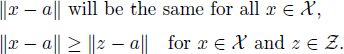
2. 2) point x is the closest to {z₁,…, z_m} among all equidistant points, i.e.

In other words, the circumcenter is the solution to the optimization problem

[A2.1]

The circumcenter may exist and may not exist, because the constraints in the optimization problem can be incompatible. However, if it exists, it is unique, as shown in the following lemma.

LEMMA A2.1.– If the constraints in optimization problem [A2.1] are compatible, problem [A2.1] has a unique solution.

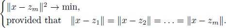
PROOF.– A point x satisfies the constraints in optimization problem [A2.1] if and only if and only if

which is equivalent to

[A2.2]

Thus, the constraint set is defined by a system of linear equations and is an affine subspace in . Since the constraint set is closed and non-empty and the criterion function is continuous and tends to , the constrained minimum exists. As the constraint set is convex and the criterion function ||x — z_m||² is strictly convex, the constrained minimum is reached at a unique point.

□

DEFINITION A2.2.– Let z₁,…, z_m be the points in . The sphere : ||z — a|| = R} of the minimal radius on which all the points z_i are located is called the circumsphere of {z₁,…, z_m}.

The circumsphere exists if and only if the circumcenter exists. The circumcenter is the center of the circumsphere.

Now find the circumcenter of {z₁,…, z_m} under the assumption that the points z₁,…,z_m are affinely independent, i.e. for , the equalities and imply that w_i =0 for all i. Let x be the solution to the problem [A2.1]. Then, x minimizes ||x — z_m||² under constraints that will be used in form [A2.2]. The Lagrange function is

where are the Lagrange multipliers. The Lagrange equation is

[A2.3]

Substitute [A2.3] into constraints [A2.2]:

[A2.4]

Denote n x (m — 1) matrix Z and m—1-dimensional vector

[A2.5]

Note that ||z_i — z_m||² is a diagonal element of the matrix Z^⊤Z. With this notation, equation [A2.4] can be rewritten as

[A2.6]

where diag(Z^⊤Z) is a vector created of diagonal elements of the matrix Z^⊤Z, and equation [A2.3] can be rewritten as

[A2.7]

Affine independence of the vectors z_i implies that the matrix Z is of full rank (this seems to be obvious; however, the formal proof is presented in section A2.2) and equation [A2.6] has a unique solution

[A2.8]

THEOREM A2.1.– If m ≥ 2 and the points z₁,…, z_m are affinely independent, then the circumcenter of {z₁,…, z_m} exists and is equal to

[A2.9]

where the matrix Z is defined in [A2.5].

PROOF.– First, we prove that the constraints in optimization problem [A2.1] are compatible. Vector defined in [A2.8] and vector x defined in [A2.7] satisfy equations [A2.3], [A2.4] and [A2.6] and constraints in problem [A2.1]. Thus, constraints in [A2.1] are compatible.

By Lemma A2.1, the solution to optimization problem [A2.1] exists. By [A2.6] and [A2.7], it satisfies [A2.9].

□

Due to Theorem A2.1, the following algorithm finds the circumcenter of points z₁,…, z_m as long as z₁,…, z_m are affinely independent. We present the algorithm in two formats: here as a sequence of steps, and in section A2.5 in pseudocode (see Algorithm A2.1).

Algorithm for finding the circumcenter of a finite set :

Step 1. If m = 1, then take the trivial solution z₁ as the circumcenter and stop.

Step 2. Create n × (m — 1) matrix

Step 3. Set

Step 4. Set . Take x as the circumcenter.

A2.2. Constrained least squares

The problem of finding a minimal-norm point in the convex hull of a finite number of affinely independent points is studied in [WOL 76], together with the algorithm for solving the problem. Another version of the algorithm is presented in [CHA 03, Section 10.3].

A point in the convex hull of a finite set {x₁,…, x_m} can be represented as with non-negative coefficients w_i, which satisfy the constraint . Finding the coefficients w_i of the minimal-norm element is regarded as the FCLS (see the definition later in this section, equation [A2.15]).

A2.2.1. Two constrained least squares problems: SCLS and FCLS

Let X be an n × m matrix with affinely independent columns. The affine independence of the columns means that

[A2.10]

Hence, be a vector.

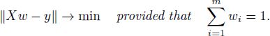
DEFINITION A2.3.– Sum-constrained least squares (SCLS) problem is the problem of finding the vector that minimizes ||Xw — y|| under the constraint :

[A2.11]

Here, ||Xw — y|| is the norm in Euclidean space, so that the norm of the vector y equals

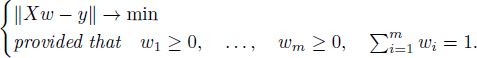
DEFINITION A2.4.– The FCLS problem is the problem of finding the vector w ∈ with non-negative elements that minimizes ||Xw — y|| under the constraint

[A2.12]

Denote x₁, x₂,…, x_m the columns of the matrix X:

If w is the solution to the SCLS problem [A2.11], then Xw is the projection of the point y onto the affine subspace spanned by the points x₁, x₂,…, x_m. If w is the solution to the FCLS problem [A2.12], then Xw is the point from the convex hull of x₁, x₂,…, x_m that is nearest to y.

Denote

[A2.13]

Then, under the constraints of either [A2.11] or [A2.12], we have

Hence, the SCLS problem [A2.11] is equivalent to

and the FCLS problem [A2.12] is equivalent to

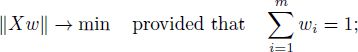
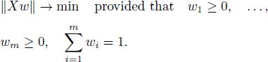
Thus, without loss of generality, we can assume that y = 0. Therefore, consider the SCLS and FCLS problems with y = 0:

[A2.14]

[A2.15]

THEOREM A2.2.– Provided that the columns of the matrix X are affinely independent, both the SCLS and FCLS problems have a unique solution.

PROOF.– First, prove the theorem for the case y = 0.

On the constraint sets (for the SCLS problem) and (for the FCLS problem), the equality (1,…, 1)w = 1 holds true, whence

Hence, the alternative criterion function

coincides with the squared criterion function ||Xw||² on the constraint sets. Since Q₁(w) is continuous and tends to +∞ as ||w|| → ∞, and the constraint sets for the SCLS and FCLS problems are closed and non-empty, the solutions to the SCLS [A2.14] and FCLS [A2.15] problems exist. Since Q₁(w) is a strictly convex set and the constraint sets are convex, the solution to any of the SCLS and FCLS problems is unique.

Let us establish that the assumption y = 0 does not lead to loss of generality. Under the constraint , we have that , where the matrix X₁ is defined in [A2.13]. Therefore, we can transform the optimization problem to an equivalent one with y = 0 by changing the matrix X. It remains to prove that if the columns of the matrix X are affinely independent, then the columns of the matrix X₁ are also affinely independent. The rest of the proof is devoted to the latter implication.

Because of the equality

[A2.16]

(where I is the n × n identity matrix, so is a non-singular matrix), the ranks of matrices in [A2.16] are equal:

We have the following equivalent properties: the matrix X has affinely independent columns if and only if

which holds true if and only if

which in turn holds true if and only if the matrix X₁ has affinely independent columns.

□

A2.2.2. SCLS algorithm

Now, construct the solution to the SCLS problem [A2.14]. Denote m×(m−1) matrix T and m-dimensional vector e_m:

Then

[A2.17]

is a representation of the vector w that satisfies the constraint from [A2.14]. Equation [A2.17] establishes one-to-one correspondence between and the constraint set

Affine independence of the columns of the matrix X implies the linear independence of the columns of the matrix XT. Indeed, we have that (1,…, 1)T = 0, whence

[A2.18]

The factors on the right-hand side of [A2.18] are matrices with linearly independent columns. Therefore, their product is also a matrix with linearly independent columns, and

Thus, XT is a full-rank matrix with linearly independent columns.

Substitute [A2.17] into [A2.14]. The resulting unconstrained minimization problem

[A2.19]

has a solution

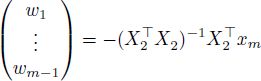
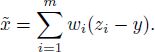
Denote

and note that X_em = x_m. Then, the minimizer in [A2.19] is equal to

[A2.20]

LEMMA A2.2.– If is the minimizer in the SCLS problem [A2.14], then all the elements of the vector X^⊤ Xw are equal.

PROOF.– Here, the notations and T are the same as above. Vector minimizes , whence

The minimizer w is represented as , whence

The null space of the matrix T^⊤ consists of m-dimensional vectors with all elements equal. Thus, all the elements of the vector X^⊤ Xw are equal.

□

Now we present the algorithm for solving problem [A2.14]. If m = 1, then the constraint set consists of a single point and the solution is trivial, i.e. w = 1. Otherwise, we solve [A2.20] and [A2.17]. It is described in Algorithm A2.2, section A2.5.

Algorithm for solving the SCLS problem to minimize ||Xw|| under constraint has the following steps:

Step 1. If X is a one-column matrix (i.e. if m = 1), then take the trivial solution w = 1 and stop.

Step 2. Construct an m—1-column matrix X₂:

where x₁,…, x_m are columns of the matrix X.

Step 3. Construct m-dimensional vector w, whose first m — 1 elements are equal to the elements of the vector

and the last element is equal to

A2.2.3. FCLS algorithm

Now we solve the FCLS problem [A2.15]. Let D be any convex set in . Also let be the projection of the set D onto jth axis.

DEFINITION A2.5.– 1) The point w₀ is called a feasible point of a minimization problem

if w₀ satisfies the constraints, i.e. if w₀ ∈ D.

1. 2) For the function and for the fixed index 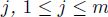, the function defined by formula

is called the profile of the function f.

The profile of a convex function is a convex function.

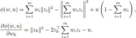
LEMMA A2.3.– The vector w is a solution to the FCLS problem if and only if the following holds true: w is the feasible point in the sense that w_i ≥ 0 for i = 1,…, m and , and the elements of the vector satisfy the condition

[A2.21]

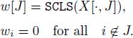
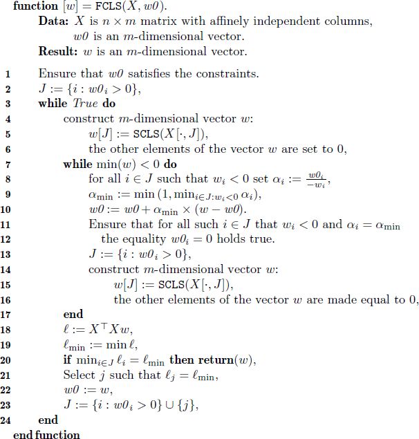
Now we present the algorithm for finding the minimizer in the FCLS problem [A2.14]. In the algorithm, letter J means the set, J ⊂ {1, 2,…, m}; X[·, J] is the submatrix of the matrix X constructed of the columns of the matrix X with indices within the set J; w[J] = (w_i, i ∈ J) is the vector made of the elements of vector w with indices within J.

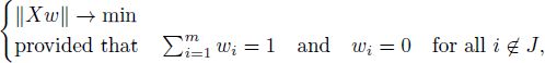
Algorithm for solving the FCLS problem [A2.15], which consists of the minimization of ||Xw|| under constraints and w_i ≥ 0 for i = 1,…, m, has the following form:

Step 1. Create an m-dimensional vector w0 that satisfies the constraints [A2.15].

Step 2. Put

Step 3. In order to find the minimizer in the problem

[A2.22]

we consider m-dimensional vector w with elements

Step 4. If all the elements of vector w are non-negative, go to step 6. Otherwise, go to step 5.

Step 5. Move w0 toward w as far as it satisfies the constraints. Make sure that after the movement, all the elements of w0 are non-negative. Also make sure that at least one element of w0 that was previously positive becomes 0. Go to step 2.

Step 6. Calculate the vector

Step 7. If the minimal element of the vector ℓ is reached for some index i ∈ J, i.e. if

then fix w as the result and terminate the algorithm. Otherwise, go to step 8.

Step 8. Select an index j such that

Step 9. Set w0 = w.

Step 10. Let the set J consist of indices i for which either w0_i > 0 or i = j:

Go to step 3.

The FCLS algorithm is presented in section A2.5 as Algorithm A2.3. In the structured representation of the algorithm, step 5 is explained in detail in lines 8–12.

THEOREM A2.3.– Let X be the matrix with affinely independent columns. If all the computations are exact, then Algorithm A2.3 ends and gives the solution to problem [A2.15].

PROOF.– First, prove that if the algorithm ends, then the vector w, which it calculates, will be the solution to the FCLS problem [A2.15]. When the algorithm ends, all the elements of vector w are non-negative,, and for vector , we have that

[A2.23]

Thus, , and vector w satisfies the constraints of optimization problem [A2.15].

Due to Lemma A2.2, all elements of the vector are equal. Since

all the elements of the vector are equal. Due to [A2.23],

whence [A2.21] follows.

Thus, vector w satisfies Lemma A2.3 and minimizes [A2.15].

Now prove that the algorithm ends. On every iteration of the inner cycle, the finite set J becomes smaller. Hence, on each iteration of the outer cycle, the inner cycle is iterated only a finite number of times. Thus, it is enough to prove that the outer cycle is iterated only a finite number of times. Below we prove this fact.

At lines 4–6 or at lines 14–16 of Algorithm A2.3 in section A2.5, w becomes the minimizer of problem [A2.22].

After the execution of line 1, w0 is a feasible point. Indeed, it is ensured that all elements of w0 are non-negative, and after line 1. On execution of line 10, w0 becomes a convex combination of its previous value and vector w, which satisfies . At line 22, we set w0 = w. Thus, the equality never becomes false.

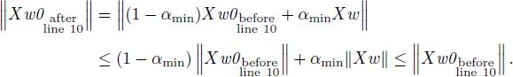
During the execution of the algorithm, ||X w0|| never increases. Indeed, after line 6 or 16, w minimizes [A2.22] while w0 satisfies the constraints in [A2.22].

Then, . We set w0 = w at line 22 and at line 10. The norm ||Xw|| is a convex function in w. Hence

Now prove that ||Xw0|| strictly decreases on each iteration of the outer cycle starting from the second one. Note that before line 23 Denote for i ∈ J on line 18 (for all i ∈ J, the elements ℓ_i of the vector ℓ are equal). After line 21, . For j obtained in line 21 and J obtained in line 23 and any denote

[A2.24]

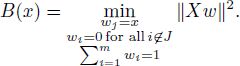
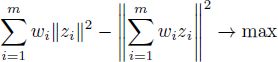
The function B(x) is convex as the profile of a convex function. If x = 0, then the minimum in [A2.24] is reached for w = w0, so that after line 21. Later on, w is redefined in lines 4–6. With tedious computations, we can prove that the derivative of B(x) at x = 0 is equal to , whence

Then, after lines 4–6

If the inner cycle is skipped, then ||Xw0|| strictly decreases on line 22. Otherwise, on the first iteration of the inner cycle 0 and ||Xw0|| strictly decreases on line 10. Thus, ||Xw0|| strictly decreases on each iteration of the outer cycle.

The vector w can reach only a finite number of different values because there are only a finite number of sets Thus, ||Xw|| can reach only a finite number of different values. After line 22, w0 = w, and because ||Xw0|| strictly decreases on each iteration of the outer cycle, ||Xw|| strictly decreases between runs of line 22. Hence, line 22 is performed only a finite number of times. The outer cycle has only a finite number of iterations, and as it was discussed earlier, the algorithm ends.

□

A2.2.4. Relation between solutions to the SCLS and FCLS problems

Here, we consider the SCLS [A2.14] and FCLS [A2.15] problems.

LEMMA A2.4.– Let X be an n × m matrix with affinely independent columns. Let w_SCLS and w_FCLS be the solutions to the SCLS and FCLS problems, respectively. Then, one of the following statements holds true:

1. 1) the equality w_SCLS = w_FCLS holds true (as a result, all the elements of the vector w_SCLS are non-negative);
2. 2) an index i exists for which w_SCLS,i < 0 and w_FCLS,i = 0.

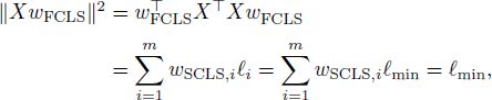
PROOF.– Assume that statement 2) does not hold true, i.e.

[A2.25]

Let us prove that statement 1) holds true, i.e. w_SCLS = w_FCLS. Indeed, by Lemma A2.2, all elements of the vector are equal. Denote ℓ_SCLS the element of . Then

[A2.26]

Denote

and

Then, by Lemma A2.3 (see equality [A2.21]),

[A2.27]

We use equalities [A2.26] and [A2.27] in the following transformations. Since , we have that

and

whence

[A2.28]

On the one hand, we can evaluate as follows:

[A2.29]

On the other hand,

[A2.30]

The inequality

[A2.31]

can be verified by considering two cases. If w_FCLS,i > 0, then [A2.31] becomes the equality due to [A2.27]. Otherwise, if w_FCLS,i = 0, then [A2.31] follows from assumption [A2.25].

It follows from [A2.28], [A2.29], [A2.30] and [A2.31] that ℓ_SCLS = ℓ_min. Hence, w_FCLS is also a solution to the SCLS problem. By Theorem A2.2, w_FCLS = w_SCLS.

□

A2.3. Dual problem

The Chebyshev center of the non-empty finite set {z₁, z₂,…, z_m} minimizes the functional

The Chebyshev center of a non-empty finite set exists and is unique (see Definition 1.2 and Corollary 1.6 in section 1.8.2).

THEOREM A2.4.– Let z₁,…,z_m and x be the points in . Then, the following statements are equivalent:

1. I) x is the Chebyshev center of {z₁, z₂,…,z_m}.
2. II) Non-negative numbers w₁,…, w_m and R exist such that:
   
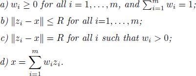
3. III) The set can be split into two subsets and (which we call the set of active points and the set of passive points) as follows:
   1. a) x belongs to the convex hull of the active set ;
   2. b) x is a center of the smallest sphere that contains the active set ; i.e. x is the circumcenter of the active points (see the definition of circumcenter in section A2.1);
   3. c) the passive points lie closer to x than the active points, i.e. the passive points lie inside or on the circumsphere of the active points.

REMARK A2.1.– In Theorem A2.4, condition III(c) means that

However, under condition III(b), this is equivalent to

In order to prove Theorem A2.4, we will verify the Karush–Kuhn–Tucker conditions, implementing this verification via the following version of the Karush–Kuhn–Tucker theorem.

THEOREM A2.5.– Let g, f₁, …, f_m be concave differentiable functions on . Suppose the following condition holds true:

[A2.32]

Then, is the maximizer of the optimization problem

[A2.33]

if and only if exists such that for the function

[A2.34]

the following conditions hold true:

[A2.35]

[A2.36]

For the proof, we refer to [KUH 51, Theorems 1, 2, and Section 8]. See also [COT 12].

REMARK A2.2.– For necessity (the “only if” part of Theorem A2.5), the concavity of the function g(x) is not needed. For sufficiency (the “if” part of Theorem A2.5), condition [A2.32] is not needed.

PROOF OF THEOREM A2.4.– The Chebyshev center is the minimizer of the function Q(y). The function Q(y) is not “everywhere” differentiable. Hence, we reduce the minimization of Q to a constrained maximization problem that involves only differentiable functions.

The maximum in is equal to the least R₂ that satisfies inequalities

[A2.37]

Therefore, among all pairs (R₂, x) that satisfy

the minimal component R₂ is equal to min Q(y), and the corresponding x is the minimizer of Q.

Thus, the problem of unconstrained minimization of Q(x) is reduced to the following constrained maximization problem:

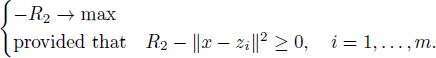
Here, we have n + 1 unknown variables: one is and the other n are the elements of the vector x.

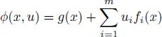
In order to describe the maximizer, we apply Theorem A2.5. The functions g and f_i are

these functions are concave and differentiable. Obviously, inequalities hold true if x = 0 and . The function φ form [A2.34] has a form

The necessary and sufficient maximality conditions are provided by Theorem A2.5. Condition [A2.35] takes the form

[A2.38]

[A2.39]

while condition [A2.36] takes the following form: for all i = 1,…,m

[A2.40]

[A2.41]

[A2.42]

Obviously, R₂ ≥ 0. Conditions [A2.38]–[A2.42] are equivalent to the conditions in statement II with . Indeed, [A2.38] and [A2.41] are equivalent to II(a), and [A2.40] is equivalent to II(b). If [A2.41] holds true, then [A2.42] is equivalent to II(c). If [A2.38] holds true, then [A2.39] is equivalent to II(d).

Now prove that statements II and III are equivalent. Suppose that statement II holds true. Split the set {z_i, i = 1,…, m} as follows. Let the active set consist of the points z_i with positive weights w_i:

Then, III(a) follows from II(a) and II(d), III(b) follows from II(c) and III(a), and III(c) follows from II(b) and II(c). Thus, statement III holds true.

Now suppose that statement III holds true. Due to III(a), x is a convex combination of elements

and W_z ≥ 0 for all . Now choose the vector w. If all z_i’s are different, i.e. if , then let

Otherwise, if some vector z appears in {z₁,…, z_m} several times, we should be careful not to assign its weight W_z to multiple w_i’s. In that case, we put

Then, II(a) and II(d) hold true.

Point x is equidistant from all active points due to III(b). Denote this distance as R. Then, II(c) holds true.

Condition II(b) follows from II(c) and III(c). Thus, statement II holds true.

□

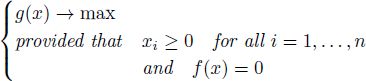
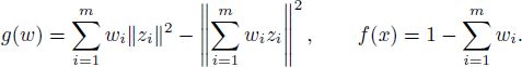
The dual optimization problem is to find the weights w₁,…, w_m that maximize the functional

[A2.43]

under the constraints

[A2.44]

If there exists a point y equidistant from z_i’s, i.e. if

then the dual problem is equivalent to minimizing the value

[A2.45]

under constraints [A2.44].

THEOREM A2.6.-

1. I) A point is the Chebyshev center of {z₁,…, z_m} if and only if non-negative numbers w₁,…, w_n exist such that:
   1. a) w₁,…, w_m maximize the functional [A2.43] under constraints [A2.44];
   2. b)
2. II) If there exists a point y equidistant from z₁,…,z_m, then a point is the Chebyshev center of {z₁,…,z_m} if and only if non-negative numbers w₁,…,w_n exist such that:
   1. a) w₁,…,w_m minimize the functional [A2.45] under constraints [A2.44];
   2. b)

In the proof of Theorem A2.6, we will use the following version of the Karush–Kuhn–Tucker theorem.

THEOREM A2.7.– Let g be a concave differentiable function , and let f be an affine function in the form for some fixed k₁,…, k_n, and h. Then, x⁰ is a maximizer of the problem

[A2.46]

if and only if u⁰ exists such that for the function

[A2.47]

the following conditions hold true

for all j = 1,…, n, and

For the proof, we again refer to [KUH 51, Theorems 1, 2, and Section 8].

PROOF OF THEOREM A2.6.– Part 1. We apply Theorem A2.7 to obtain a system of equations and inequalities that is equivalent to constrained maximization problem [A2.43]–[A2.44]. We have

Note that the function g is concave and the function f is affine. Function φ from [A2.47] and its partial derivatives equal

The necessary and sufficient optimality conditions now have a form:

[A2.48]

Conditions [A2.48] can be rewritten as follows: exists such that:

Since

with not depending on k, the optimality conditions (a)–(c) are equivalent to the following: C ≥ 0 exists such that:

With C = R² and , conditions (a’)–(c’) are the same as in part II of Theorem A2.4, which provides necessary and sufficient conditions for the point x to be a Chebyshev center.

Part 2. The point x minimizes the functional if and only if point minimizes the functional

Due to part 1 of the present theorem, minimizes if and only if there exist weights w₁,…, w_m that maximize

[A2.49]

under constraint [A2.44], and

[A2.50]

Due to the equidistance condition for all i = 1,…,m and the equality , we have

Hence, the constrained maximization of [A2.49] is equivalent to the constrained minimization of [A2.45]. Under the constraints, equality [A2.50], i.e.

holds true if and only if

□

A2.4. Algorithm for finding the Chebyshev center

We slightly modify the algorithm presented in [BOT 93]. As a prerequisite, we will require that the input points are affinely independent. During the computation, point a will stand for the approximation to the Chebyshev center, and will be the current active set. The active points will be equidistant from a, and the passive points are located not further, i.e.

The circumcenter of the active set will be denoted by o. It will be a projection of the current approximation a onto the hyperplane spanned by the active set. However, it may or may not lie in the convex hull of the active set.

In our algorithm for finding the Chebyshev center, two steps are used several times. In the deflate step, the approximation a is moved towards o as long as the largest distance between the approximation and passive points does not exceed the distance between the approximation and active points. In the other step, unnecessary points are removed from the set of active points.

A2.4.1. Deflate step

Recall the conditions that hold true during the process of the Chebyshev center algorithm:

• – is the fixed finite set, consisting of affinely independent points, the circumcenter of which we are evaluating;
• – is the set of active points;
• – the points o and a are equidistant from the active points (i.e. ||o – x|| is the same for all , and ||a — x|| is also the same for all );
  • – o is the circumcenter of ;
  • – o and a satisfy the inequality

[A2.51]

In the deflate step, we try to reduce (where x is an arbitrary point of the set ), keeping the conditions satisfied.

The set of points equidistant from the active points is an affine subspace, which is orthogonal to the affine subspace spanned by the active points, see the proof of Lemma A2.1. As a result, all the points of the segment [o, a] = are equidistant from the active points, i.e.

and vectors a — o and x — o are orthogonal, i.e. for all .

In the following, is some active point. The norms ||x — o||, ||x — a|| and ||o + λ(a − o)−x|| do not depend on x, so it does not matter which active point is chosen.

Find the point from the segment [o, a] for which ||a_new—x|| is minimal while inequality [A2.51] holds true. Since

the norm ||a_new — x|| decreases as λ ≥ 0 decreases. Hence, we find the minimal λ ≥ 0 for which

[A2.52]

Then, take a_new = o + λ(a — o) as the new value for a.

For a given , the inequality

is equivalent to

[A2.53]

Note that due to [A2.51], inequality [A2.52] holds true for λ = 1. Therefore, inequality [A2.53] holds true for λ = 1 and for all .

Now solve inequality [A2.53] for λ ∈ [0,1]. Consider three cases. If , then [A2.53] holds true for all λ ∈ [0,1], because it holds true for λ = 1. If and , then obviously [A2.53] holds true for all λ ∈ [0,1]. Otherwise, if and ||z — o||² — ||x — o||² > 0, then [A2.53] holds true for all

For fixed λ ∈ [0,1], inequality [A2.52] is satisfied if and only if inequality [A2.53] is satisfied for all , which is equivalent to

where K is a subset of ,

Note that .

If , then the minimal λ ∈ [0,1] for which [A2.52] holds true is 0. If then minimal λ for which [A2.52] holds true is

[A2.54]

In the former case, optimal a_new coincides with o. In the latter case, for with λ defined in [A2.54], for at least one z ∈ K the equality ||a_new — z|| = ||a_new — x|| holds true.

In the deflate step, we perform the following:

• – move a towards o as close as possible without ruining inequality [A2.51];
• – if the new point a does not coincide with o (this is the case , include points z ∈ K for which ||a — z|| = ||a — x|| into the active set ;
• – adjust the circumcenter o according to the new active set .

The algorithm of the deflate step is the following:

Step 1. Find the set and ||z — o||² — r² > 0}, where r² = ||x — o||² for all x ∈ X (the value of ||x — o||² does not depend on the choice of x ∈ X is used).

Step 2. If , put a := o and stop.

Step 3. For every z ∈ K, evaluate

Step 4. Put

Step 5. Ensure that λ_max ∈ [0,1]. Hence, if λ_max > 1 (which cannot occur if all the computations were exact, but may occur due to computational errors), then put λ_max := 1.

Step 6. Put

Step 7. Include into the active point set the element (or the elements) z ∈ K for which was adjusted in step 5):

Step 8. Evaluate the circumcenter of the active set and assign its value to o.

Then a, and o are the results. This is Algorithm A2.4 presented in section A2.5 in pseudocode.

Note the following fact: either the active point set does not change in the deflate step and a = o after the step, or the active point set strictly increases in the deflate step.

A2.4.2. Two algorithms for the evaluation of the Chebyshev center

In this section, we present two algorithms for the evaluation of the Chebyshev center of an affinely independent set . The affine independence makes the evaluation of the circumcenter of the input points (or of any of their subset) well defined.

Once we have Circumcenter and FCLS algorithms available, we can find the algorithm as follows.

The first algorithm for finding the Chebyshev center of an affine independent set is as follows:

Step 1. Find the circumcenter of the set :

Step 2. Construct the matrix

where z₁,…,z_m are the elements of the set .

Step 3. Choose an arbitrary vector w0 that satisfies the constraints [A2.44].

Step 4. Solve the FCLS problem:

Step 5. Put The point a is the Chebyshev center.

The weights evaluated in step 4 constitute the solution to the dual problem (see Theorem A2.6). As a result, the algorithm evaluates the Chebyshev center as expected.

The drawback of this algorithm is its instability if the points z_i are nearly affinely dependent. In this case, the circumcenter o can be a distant point, which may affect the precision of computation.

Hence, we propose another algorithm for finding the Chebyshev center. The inputs for this algorithm are the initial approximation a and the finite set The outputs are the Chebyshev center a and the final set of active points .

The second algorithm for finding the Chebyshev center of an affine independent set is as follows:

Step 1. Initialize the set of active points. It will consist of the point of , which are the most distant from the a:

Step 2. Evaluate the circumcenter of the active points:

Step 3. Repeat the deflate step

until a = o.

Step 4. Evaluate the weights in the convex combination o = . To do this, construct the matrix X_o of the form

where x₁,…, x_p are the elements of the active set and p is the number of elements in . Then, apply the SCLS algorithm:

Step 5. If all the elements of the vector w_SCLS are non-negative, take a as the Chebyshev center, as the final set of active points and stop.

Step 6. Solve the FCLS problem. Construct a vector w0 of the initial approximation:

Then, put

Step 7. In Lemma A2.4, the second alternative holds true. An index i exists such that w_SCLS,i < 0 and w_FCLS,i = 0. (Choose one if these hold true for multiple i’s.) Remove the point x that corresponds to such i from the active set . Go to step 2.

It is Algorithm A2.5 presented in pseudocode in section A2.5.

During the execution of the algorithm, the inequality

holds true. When the algorithm ends, a = o is a convex combination of the active points; moreover, it is the circumcenter of the set of the active points. By Theorem A2.4, a is the Chebyshev center of the set .

A2.5. Pseudocode of algorithms

Now we transform the algorithms previously presented as a sequence of steps into pseudocode in order to allow the reader to implement them in a structured programming language.

Algorithm A2.1.– Pseudocode of the algorithm for finding the center of the circumscribed sphere of a finite set (see the sequence of steps in section A2.1).

ALGORITHM A2.2.– Pseudocode of the algorithm for solving the SCLS problem (see the sequence of steps in section A2.2.2).

The lines of the following algorithm are referenced in the proof of Theorem A2.3.

ALGORITHM A2.3.– Pseudocode of the algorithm for solving the FCLS problem (see the sequence of steps in section A2.2.3).

Here, “Ensure that … the equality w0_i = 0 holds true” means the following. If computations are performed with errors, then set w0_i = 0. Otherwise, if all computations are exact, then do nothing.

ALGORITHM A2.4.– Pseudocode of the deflate step of the Chebyshev center algorithm (see the sequence of steps in section A2.4.1).

ALGORITHM A2.5.– Pseudocode of the second algorithm for finding the Chebyshev center (see the sequence of steps in section A2.4.2).