
Chapter 8
Solve That Problem
Computers are universal machines that can be programmed to perform almost any task. They allow us to automate solutions to problems. Such solutions can be performed by computers repeatedly, reliably, precisely, and with great speed. Not all problems lend themselves to automated solutions. But CT demands that we try to find solutions that can be automated.
The stages of computer automation are conceptualization, algorithm design, program design, and program implementation. In other words, programmers must devise solution strategies, implement algorithms, and write program code to achieve the desired results.
Specifying and implementing solution algorithms requires precise and water-tight thinking. Also required is anticipation of possible input as well as execution scenarios. Few are born with such talents. But, we all can become better problem solvers by studying cases, experimentation, and building our solution repertoire.
Often, there are multiple algorithms to solve a particular problem or to achieve a given task. Some may be faster than others. Some may use fewer resources. Others may be easier to program or less prone to mistakes. Analyzing and comparing different solution algorithms is an important part of problem solving.
Usually, we are after the fastest algorithm or one that uses the least amount of memory space. Problem-solving skills from computing can be useful in other areas, as well as in our daily lives.
8.1 Solving Puzzles
A good way to begin thinking about problem solving is perhaps by looking at a few puzzles.
8.1.1 Egg Frying
The Problem: A pan can fry up to two eggs at a time (Figure 8.1). We need to fry three eggs. Each egg must be fried for one minute on each side. Design an algorithm to fry the three eggs in as little pan-frying time as you can manage.
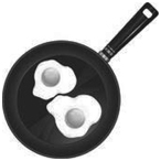
FIGURE 8.1 Egg Frying
The slowest method would fry one egg at a time, cooking each side for one minute. It would take a total of six minutes of pan-frying time.
A better method would fry two eggs, turning them over after a minute, and cook for another minute. After that, fry the third egg. This method takes a total of four minutes.
Is this the best we can do? Well, no. We can do better:
- Start with frying two eggs for one minute.
- Take one of the half-done eggs out of the pan, turn the other egg over, and add the third egg in the pan, fry for one minute.
- Take out the egg that is done, flip the other egg over, and add back the half-done egg, fry for one minute.
- Take both eggs out and terminate.
Each step takes one minute. The whole procedure takes three minutes to get the job done.
Again, is this the best we can do? Well, yes. How do we know? Can we prove that no method can be faster?
Here is a proof. The three eggs require six egg-side-minutes of frying. The pan can supply a maximum of two egg-side-minutes per minute. Thus, at least three minutes are needed to produce six egg-side-minutes, no matter how the frying is done.
8.1.2 Liquid Measuring
The Problem: We have a 7-oz cup and a 3-oz cup (Figure 8.2). Unfortunately, neither has any volume markings on it. We have a water faucet, but no other containers. Find a way to measure exactly 2 ounces of water.

FIGURE 8.2 Two Cups
We see the allowable operations are filling water from the faucet, pouring water from one cup to the other, and emptying the cups. Here is how we can proceed:
- Fill the 3-oz cup completely.
- Empty the 3-oz cup into the 7-oz one.
- Repeat steps 1 and 2 one more time.
- Fill the 3-oz cup again completely.
- Pour water from the 3-oz cup into the 7-oz cup until it is full.
- Two ounces of water now remain in the 3-oz cup.
What about measuring 5 or 6 ounces of water? If we switch the 7-oz cup to an 8-oz cup, can you solve the same problem? What if we switch it to a 6-oz cup? Try Demo: LiquidMeasure at the CT site.
8.1.3 A Magic Tray
The Problem: A magic tray is a perfect square and has four corner pockets (Figure 8.3) whose openings look exactly the same. Inside each pocket is a cup hidden from view. The tray also has a green light at the center.
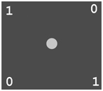
FIGURE 8.3 Magic Tray Puzzle
Cups inside the pockets can be either up (1) or down (0). The light will turn red automatically if all four cups are in the same orientation.
Your job is to turn the light red by performing a number of steps. Each step consists of reaching into one or two pockets to examine and optionally reorient the cups. No other operations are allowed. Remember, you can’t see the cups. Figure 8.3 shows one possible configuration to give you an idea.
To complicate things, the tray immediately spins wildly after each step. When it stops spinning, there is no way to tell which pockets you had examined in the last step.
Your job is to create an algorithm to turn the light red, no matter what the initial orientations of the cups are. Remember, an algorithm must specify exactly what to do at each step and guarantee termination after a finite number of steps. Therefore, keep reaching into pockets and turning cups up (or down) is not a solution because you may be extremely unlucky and reach into the same pockets every time.
One observation we can make is that we may choose to reach into pockets along a side or on a diagonal. But there is a chance, however small, that we may reach into the same side/diagonal all the time. Our algorithm must work even if it never ever examines all four pockets. This puzzle is fun and hits home the algorithm ideas perfectly. We will leave the reader to work out this algorithm. It should take no more than 7 steps. See Exercise 8.1 for a hint and Demo: MagicTray at the CT website for a solution.
8.2 Sorting
In automated data processing, the need to arrange a list of items into order often arises. In computer science, to sort is to arrange data items into a linear sequence (in memory) so individual items can easily be retrieved. In fact, we have seen the binary search algorithm for efficient retrieval from a sorted list (Section 1.8).
Sorting is a major topic in algorithm design. Many ways have been devised and research papers published for sorting.
8.2.1 Bubble Sort
Let’s present here the most basic bubble sort algorithm. We shall see how bubble sort rearranges the n elements of a sequence a 0 , an, ..., a n-1 to put them into ascending order:
Bubble sort performs a number of compare-exchange (CE) operations. Each compare-exchange operation compares two adjacent elements of the sequence, and exchanges them if necessary so the latter element is larger. Here is the pseudo code for exchanging any two values x and y.
Algorithm exchange(x,y) :
Input: Integer x, integer y
Effect: Values of x, y exchanged
- Set temp = y
- Set y = x
- Set x = temp
To describe bubble sort, let’s see how it sorts a sequence of eight elements, a 0, a2, ···, a7. Pass 1 performs seven CE operations (Figure 8.4): CE(a0, a1), CE(a1, a2), CE(a2, a3), CE(a3, a 4 ), CE(a4, a5), CE(a5, a6), and CE(a6, a7).

FIGURE 8.4 Bubble Sort
In a similar manner, pass 2 moves the largest value of a0, a1, ..., a 6 up into a 6 ; pass 3 moves the largest value of a0, a1, ..., a5 up into a5; and so on, until, finally, pass 7 moves the the largest value of a 0 and a 1 into a 1 to complete the sorting.
Let’s put bubble sort in an algorithmic form (CT: MAKE IT AN ALGORITHM, Section 1.8). The bubble sort pseudo code, using for loops (Section 3.5.2), is as follows:
Algorithm bubblesort:
Input: Array of integers a[0] ... a[n–1] and the array length n
Effect: The array elements are rearranged in ascending order
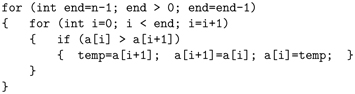
Note the CE operation in the body of the inner loop.
So how efficient is bubblesort? For the 8-element case, pass 1 performs 7 CE operations, pass 2 performs 6 CE operations, and so on. Thus, for sorting 8 elements, bubblesort performs:
CE operations. In general, for sorting n elements, bubblesort performs
CE operations.
8.2.2 Improved Bubble Sort
One of the basic activities in computing is finding more efficient ways to do things and to make improvements to the procedures we already have. Take the bubblesort in Section 8.2.1, for example. For any given input sequence of length n, it always requires CE operations, even if the given sequence is already in order!
For any algorithm, an input that causes the most number of operations is called a worst case. With bubble sort, the worst case, where the given sequence is in descending order, does require CE operations. But, can we do better in less bad cases?
Sure we can. Observe that for any single pass, if no exchange is done after CE on the first two elements, then the sequence is already in order and we can terminate the procedure. Let’s refer to this as the in-sequence condition.
We can modify the for loop in algorithm bubblesort to incorporate this improvement.

A logical variable go_on, originally set to true, is used to control the outer for loop. Immediately before each pass, go_on is set to false. Any exchange operation where i is greater than 0 causes go_on to become true. The go_on being false stops the looping from proceeding to the next pass. Trace the code and satisfy yourself that it works.
Before discussing more examples, let’s first give some general principles and approaches for problem solving.
CT: CUT IT DOWN
Solve a problem by reducing it to increasingly smaller and simpler problems.
For example, bubble sort chips away at the problem. With each pass, the length of the sequence to be sorted is reduced by one. And repeated chipping soon gets the job done.
When solving a problem, we generally have two approaches, the top-down approach and the bottom-up approach. Top-down problem solving involves taking a big and complicated problem and breaking it down into several smaller subproblems (divide and conquer). Each subproblem can either be solved directly or be broken down further. When all the subproblems are solved, the big problem is finished.
CT: BUILD IT UP
Combine basic known quantities and methods to build ever larger and more complicated components that can be applied to solve problems.
In contrast, the bottom-up approach of problem solving starts from given data, known quantities, and methods to build up components which can be combined to achieve a particular task or problem solution. The way modern digital computers work is a good example of the bottom up approach. Bits plus their basic logic operations (logic gates) combine to represent and manipulate data, eventually leading to programs that can solve all kinds of problems. The LEGO® toy is an excellent example of the bottom-up approach.
When trying to solve a problem, we often need to apply top-down as well as bottom-up thinking. Breaking the given problem down while also combining known data and techniques up can often help us find solutions.
CT: STEPWISE REFINEMENT
Set up the overall problem solving strategy and how different parts of the solution interact/cooperate. Make it work first. Then make improvements in the various steps to fine tune the algorithm or program.
When specifying the solution algorithm or implementing a program, it is easy to get lost in the details and not see the forest for the trees. The stepwise refinement methodology in computer science suggests that we focus on the big picture and get the solution framework going correctly first. Once we have a working algorithm/program, we can find many places to make refinements for better speed and efficiency.
Adding the in-sequence condition improvement to the basic bubble sort algorithm is an example. We’ll see more such examples later. However, we must understand at the same time, no amount of stepwise refinement can rescue an inefficient algorithm such as bubble sort.
CT: VERSION 2.O
Taking advantage of user experience and feedback, software evolves and improves constantly with time. So should we in what we do in our daily lives.
Every time we download an application update or purchase the next version of an operating system, it reminds us of the idea of “constant improvement.” For companies, organizations, and individuals, the question is, “Are you improving? Where is your version 2.0?”
8.3 Recursion
A circular definition is usually no good and to be avoided, because it uses the terms being defined in the definition, directly or indirectly. For example Bright: looks bright when viewed. Or Adult: person not a child and Child: person not an adult. A circular definition is like a dog chasing its tail. It goes on and on to no end. However, a term or concept can be defined recursively when the definition contains the same term or concept without becoming circular. A recursive definition has base cases that stop the circling at the end. For people first exposed to recursion, the concept can be confusing. But, it is simple once you understand it. Please read on.
In mathematics, a recursive function is a function whose expression involves the same function. For example, the factorial function
can be recursively defined as
For n =1, 1! = 1 (base case)
For n > 1, n! = n x (n — 1)! (recursive definition)
In computing, a recursive function or algorithm calls itself either directly or indirectly. Here is the pseudo code for a recursive factorial function.
Algorithm factorial(n) :
Input: Positive integer n
Output: Returns n!
- If n is 1, then return 1
- Return n x factorial(n–l)
The “return” operation terminates a function and may also produce a value. Step 2 returns the value n times the value of factorial(n–l), which is a call to the same function itself (Figure 8.5).

FIGURE 8.5 Recursive Calls and Returns
To solve a problem recursively, we reduce it to one or more smaller problems of the same nature. The smaller cases can then be solved by applying the same algorithm recursively until they become simple enough to solve directly.
CT: REMEMBER RECURSION
Think of recursion when solving problems. It can be a powerful tool.
To appreciate the power of recursion and to see how it is applied to solve nontrivial problems, we will study several examples.
Greatest Common Divisor
Consider computing the greatest common divisor (GCD) of two non-negative integers a and b, not both zero. Recall that gcd(a, b) is the largest integer that evenly divides both a and b. Mathematics gives gcd(a, b) the recursion
- If b is 0, then the answer is a
- Otherwise, the answer is gcd(b, a mod b)
Recall that a mod b is the remainder of a divided by b. Thus, a recursive algorithm for gcd(a, b) can be written directly:
Algorithm gcd(a,b):
Input: Non-negative integers a and b, not both zero
Output: The GCD of a and b
- If b is zero, return a
- Return gcd(b, a mod b)
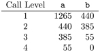
Note, the algorithm gcd calls itself, and the value for b gets smaller for each successive call to gcd (Table 8.1). Eventually, the argument b becomes zero and the recursion unwinds: The deepest recursive call returns, then the next level call returns, and so on until the first call to gcd returns.
TABLE 8.1 Recursion of gcd(1265,440) = 55
8.3.1 Quicksort
Another good example of recursive algorithms is the quicksort. Among many competing sorting algorithms, quicksort remains one of the fastest. It is much faster than bubble sort, which is not used in practice.
Let us consider sorting an array of integers into increasing order with quicksort. The idea is to split the array into two parts, smaller elements to the left and larger elements to the right. This is the partition operation, which first picks any element of the array as the partition element 1 , pe. By exchanging elements, the array can be arranged so all elements to the right of pe are greater than or equal to pe. Also, all elements to the left of pe are less than or equal to pe. The location of pe is called the partition point.
After partitioning, we have two smaller ranges to sort, one to the left of pe and one to the right of pe. The same method is now applied to sort each of the smaller ranges. When the size of a range becomes less than 2, the recursion terminates.
Algorithm quicksort(a, i, j):
Input: Array a, start index i, end index j
Effect: Elements a[i] through a[j] in increasing order
- If i greater than or equal to j, then return;
- Set k = partition(a, i, j)
- quicksort(a, i, k–1)
- quicksort(a, k+1, j)
Algorithm quicksort performs sorting on a range of elements in the array a. The range starts with index i and ends with index j, inclusive. To sort an array with 8 elements, the call is quicksort(a, 0, 7).
The algorithm starts with the base case: If i > j, the range is either empty or contains a single element, and there is nothing to do and the algorithm returns. If j is bigger than i, a partition operation is performed to split the range into two parts, as described earlier. The pe has found its final position on the array at index k. Then, quicksort is called recursively to sort each of the two smaller arrays on either side of the pe.

FIGURE 8.6 Partition in Quicksort
The partition function receives the array a and two indices, low and high, as input and performs these three steps.
- Picks a pe in the given range of elements, randomly or by some simple criteria. Exchange pe with a[high] so that pe is saved at the end of the range (Figure 8.6 A).
- Searches from both ends of the range (low, high-1) toward the middle for elements belonging to the other side, interchanging out-of-place entries in pairs, resulting in the configuration shown in Figure 8.6 B.
- Exchanges pe with the element at the partition point (Figure 8.6 C) and returns the pe index (k).
The pseudo code, using while loops (Section 3.5.1), for the partition function, can also be given.

In the unfortunate case where pe happens to be the largest (smallest) element in the range low to high, the partition position becomes high (low), and the split is not very effective. The split becomes more effective when the two subproblems are of roughly equal size (See Exercise 8.5).
Quicksort is efficient in practice, because it often reduces the length of the sequences to be sorted quickly. Note also that quicksort performs the reordering in place. No auxiliary array, as required by some other sorting algorithms, is used. The best way to understand how quicksort works is to try an example with less than 10 entries by hand.
8.4 Recursive Solution Formula
CT: APPLY THE RECURSION MAGIC
Answer two simple questions and you may have magically solved a complicated problem.
For many, recursion is a new way of thinking and brings a powerful tool for problem solving. To see if a recursive solution might be applicable to a given problem, you need to answer two questions:
- Do I know a way to solve the problem in case the problem is small and trivial?
- If the problem is not small or trivial, can it be broken down into smaller problems of the same nature whose solutions combine into the solution of the original problem?
If the answer is yes to both questions, then you already have a recursive solution!
A recursive algorithm is usually specified as a function that calls itself directly or indirectly. Recursive functions are concise and easy to write once you recognize their basic structure. All recursive solutions use the following sequence of steps.
- Termination conditions: Always begin a recursive function with tests to catch the simple or trivial cases (the base cases) at the end of the recursion. A base case (array size zero for quicksort and remainder zero for gcd) is treated directly and the function returns.
- Subproblems: Break the given problem into smaller problems of the same kind. Each is solved by a recursive call to the function itself passing arguments of reduced size or complexity.
- Recombination of answers (optional): Finally, take the answers from the subproblems and combine them into the solution of the original bigger problem. The function call now returns. The combination may involve adding, multiplying, or other operations on the results from the recursive calls.
For problems, like the GCD and quicksort, where no recombination is necessary, this step becomes a trivial return statement. However, in the factorial solution, we need to multiply by n the result of the recursive call factorial(n–1).
The recursion engine described here is deceptively simple. The algorithms look small and quite innocent, but the logic can be mind-boggling. To illustrate its power, we will consider the Tower of Hanoi puzzle.
8.5 Tower of Hanoi
Legend has it that monks in Hanoi spend their free time moving heavy gold disks to and from three poles made of black wood.
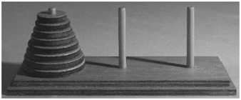
FIGURE 8.7 Tower of Hanoi Puzzle
The disks are all different in size and are numbered from 1 to n according to their sizes. Each disk has a hole at the center to fit the poles. In the beginning, all n disks are stacked on one pole in sequence, with disk 1, the smallest, on top, and disk n, the biggest, at the bottom (Figure 8.7). The task at hand is to move the disks one by one from the first pole to the third pole, using the middle pole as a resting place, if necessary. There are only three rules to follow:
- A disk cannot be moved unless it is the top disk on a pole. Only one disk can be moved at a time.
- A disk must be moved from one pole to another pole directly. It cannot be set down some place else.
- At any time, a bigger disk cannot be placed on top of a smaller disk.
To simplify our discussion, let us label the first pole A (source pole), the second pole B (the parking pole), and the third pole C (the target pole). If you have not seen the solution before, you might like to try a small example first, say, n = 3. It does not take long to figure out the following sequence.
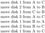
So it turns out that you need 7 moves for the case n = 3. As you get a feel of how to do three disks, you are tempted to do four disks, and so on. But you will soon find that there seems to be no rule to follow, and the problem becomes much harder with each additional disk. Fortunately, the puzzle becomes very easy if you think about it recursively.
Let us apply our recursion engine to this puzzle in order to generate a sequence of correct moves for the problem: Move n disks from pole A to C through B.
- Termination condition: If n =1, then move disk 1 from A to C and return.
- Subproblems: For n > 1, we shall do three smaller problems:
- Move n — 1 disks from A to B through C
- Move disk n from A to C
- Move n — 1 disks from B to C through A
There are two smaller subproblems of the same kind, plus a trivial step.
- Recombination of answers: This problem is solved after the subproblems are solved. No recombination is necessary.
Let’s write down the recursive function for the solution. Two recursive calls and a move of disk n is all that it takes.
Algorithm hanoi(n, a, b, c):
Input: Integer n (the number of disks), a (name of source pole), b (name of parking pole), c (name of target pole)
Output: Displays a sequence of moves
- If n = 1, display “Move disk 1 from a to c” and return.
- hanoi(n-1, a, c, b)
- Display “Move disk n from a to c”
- hanoi(n-1, b, a, c)
Each of steps 2 and 4 makes a recursive call. This looks almost too simple, doesn’t it? But it works. To obtain a solution for 7 disks, say, we make the call
hanoi(7, ‘A’, ‘B’, ‘C’)
During the course of the solution, different poles are used as the source, middle and target poles. This is the reason why the hanoi function has the a, b, c parameters in addition to n, the number of disks to be moved at any stage. Figure 8.8 shows the three-step recursive solution for n = 5:
- Move 4 disks from pole A to pole B (hanoi(4, ‘A’, ‘C’, ‘B’))
- Move disk 5 from pole A to pole C
- Move 4 disks from pole B to pole C (hanoi(4, ‘B’, ‘A’, ‘C’))
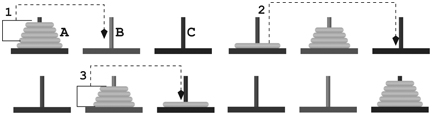
FIGURE 8.8 Tower of Hanoi (Five Disks)
Now, what is the number of moves needed for the hanoi algorithm for n disks? Let the move count be mc(n). Then we have:
- If n = 1, then mc(n) = 1.
- If n > 1, then mc(n) = 2 x mc(n — 1) + 1
The above definition for mc(n) is in the form of a recurrence relation, and it allows us to compute mc(n) for any given n.
But, we can also seek a close-form formula for mc(n)
Generally:
An interactive Tower of Hanoi game (Demo: Hanoi) can be found at the CT website. Because 2 n — 1 moves will be needed for n disks, you should test the program only with small values of n. But the monks in Hanoi are not so fortunate, they have 200 heavy gold disks to move, and the sun may burn out before they are finished!
But the logic behind the recursion engine provides a problem solving strategy unparalleled by other methods. Many seemingly complicated problems can be solved easily with recursive thinking.
8.6 Eight Queens
The Bavarian chess player Max Bezzel formulated the Eight Queens problem in 1848. The task is to place eight queens on a chess board so that no queen can attack another on the board. As you may know, a queen can attack another piece on the same row, column, or diagonal. And the question is how many solutions are there.
It turns out that there are 12 basic solutions (Figure 8.9 shows one). Other solutions can be derived from these by board rotations or mirror reflections for a total of 92 distinct solutions.

FIGURE 8.9 Eight Queens
We know a necessary condition for a solution is that each column and each row must contain one and only one queen. To satisfy this necessary condition, there are 8 possible column positions for row 1, 7 for row 2, and so on, for a total of 8! = 40320 queen placements. A brute-force way to find solutions is to check all 8! cases for diagonal attacks.
But we can do better than that by using a solution technique called backtracking. The idea is to place the queens, one at a time, making sure the next queen is placed in a nonattacking position in relation to previously placed queens. If the procedure finished placing all 8 queens, we have a solution. If it got stuck along the way, we backtrack to the previous queen and move it to its next possible position. If it has no next position, then we backtrack further. Compared to the brute-force method, backtracking examines far fewer cases.
To illustrate backtracking, let’s look at a Four Queens problem. We begin by placing the first queen in the first column at board position (1,a) (Figure 8.10 left). Next we place our second queen in the second column at board position (3,b). We then found that there is no place for the third queen in the third column. We are stuck.

FIGURE 8.10 Four Queens Backtracking
So, we go back and move the second queen to the next possible position in the column at board position (4,b). This allows us to place the third queen in the third column at position (2,c), only to find there is no position for the fourth queen (Figure 8.10 middle).
Again, we need to go back and change the position of a previous queen. It turns out that we have no next positions for the third or second queen. We are forced to move the first queen to its next possible position (2,a). From this position, proceeding in the same manner as before, we finally arrive at a solution (Figure 8.10 right). This is clearly faster than the brute-force approach. The efficiency of backtracking comes from abandoning further queen placements after getting stuck.
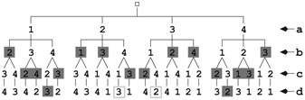
FIGURE 8.11 A Solution Tree
To illustrate the savings, let’s look at the solution tree (CT: LEARN FROM TREES, Section 4.8.2) for the Four Queens problem (Figure 8.11), where the first level nodes give the row positions for the first queen (in column a on the board), the second level positions for the second queen (column b), and so on.
The solid shaded nodes are deadends. The paths leading to the two boxed nodes represent the only two solutions. You can see in Figure 8.11 how many tree branches are pruned by backtracking, resulting in significant computational savings.
Backtracking Implementation
Let’s see how backtracking is applied to solve the Eight Queens problem by showing an algorithm for it. Our algorithm uses the following quantities:
- The size of the board is N by N; both rows and columns are numbered from 1 to N
- The integer array qn, with elements qn[0] through qn[N]
- The quantity qn[c] is the row position of the queen in column c, where 1 < c < N
The backtracking algorithm attempts to position a queen in each successive column and is specified as a recursive function queens:
Algorithm queens(r0, c):
Input: Integer r0 (starting row), c (current column)
Effect: queens(1,1) displays all solutions for the N queens problem
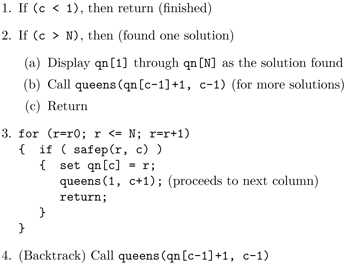
After setting N=8, the call queens(1, 1) produces all 92 solutions for the Eight Queens problem.
The function terminates (Step 1) if c is zero (backtracked to the left of column 1). Otherwise (Step 2), if c exceeds N (a queen in each column), it displays the solution and continues (Step 2b) to check for more solutions before returning.
When Step 3 is reached, the function tries to place a queen in column c at a valid row between r0 and N inclusive. After each successful row placement, it continues to the next column by calling queens(1, c+1). Finally (Step 4), having processed all rows between r0 and N, it backtracks to the previous column for more solutions.
The predicate safep checks the validity of position (r, c) for placing a queen and returns true or false.
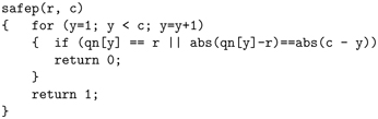
The function makes sure that the position (r, c) is not on an occupied row or diagonal by a queen in an earlier column.
See an interactive Demo: Queens at the CT site, where you can place queens on a board to find solutions interactively, and also see all 92 basic solutions for the Eight Queens problem.
8.7 General Backtracking
We used the Eight Queens problem to introduce the backtracking technique, which is generally applicable to solve problems by building a solution one element at a time. For a queens problem, we can place one queen at a time until all queens are placed. Other such problems include crossword and Sudoku puzzles. But backtracking is not just for games. It has wide applicability in solving practical problems, such as the knapsack problem, packing items of different weight or size into a container. The goal is to maximize the total dollar value, for example, of the packed items.
Similar to the queens problem, the knapsack problem is a type of combinatorial optimization problem where different combinations of items, satisfying given conditions known as constraints, are examined to optimize certain desired values. For the queens problem, we have the nonattacking constraint, and we want to find different ways to place the maximum number of queens on the board. For the knapsack problem, we want to find different ways to pack the given items in order to maximize the value of the packed items under certain measures.
8.8 Tree Traversals
We have talked about the organization of computer files in Section 4.8.2, where Figure 4.6 showed a typical file tree. A tree is a very useful way to organize hierarchical data (CT: LEARN FROM TREES, Section 4.8.2). Family trees are well-known. Internet domain names are also organized into a tree structure.

FIGURE 8.12 Windows File Search
On a computer, sometimes we need to search for a file because we have forgotten its folder location, or we are not sure of the file’s precise name. Or, we want to find all files whose name contains a certain character string. Most operating systems provide a way for users to do such searches. It can be as easy as typing in a substring of the file name (Figure 8.12) and a computer program will look for files with matching names in the entire file tree. This is very convenient, indeed. In fact, you can also find files containing certain words. That can come in handy when you remember parts of the file contents but not the file name.
But, how can such search operations be performed? Well, we need a systematic way to visit each node on the file tree, known as a tree traversal. A file tree traversal enables a program to visit all files, following folders and subfolders, and to match file names or contents with user input.
The two most common tree traversal algorithms are depth-first traversal (dft) and breadth-first traversal (bft). With bft, we visit the root, then its child nodes, then grandchild nodes, and so on. With dft, we visit the root, then we dft the first child branch, dft the 2nd child branch, and so on. Figure 8.13 shows the node-visit order for a tree using bft and dft.
Implementation of the bft is straightforward. Because dft is defined recursively, we can use a recursive algorithm to implement it.
Algorithm dft(nd):
Input: nd the starting node for dft traversal
Effect: visiting every node in the tree rooted at nd in dft order

FIGURE 8.13 Tree Traversals
- Visit nd
- If nd is a leaf node (no children), then return
- Otherwise, for each child node c of nd, from first child to last child, call dft(c)
Trace this algorithm when called on the root of the tree in Figure 8.13 and verify the dft order given in the figure.
CT: FORM TREE STRUCTURES
Keep the tree structure in mind. It can be found everywhere and can be used to advantage in many situations.
Let’s take a fresh look at the solution tree (Figure 8.11) for the Four Queens problem in Section 8.6. We see now that the backtracking algorithm employed there is simply a dft of the solution tree while applying the nonattacking condition at each node. A solution is found whenever a valid last level leaf is reached.
Tree traversal is important in programming because tree structures are found in many varied situations. For example, markup languages, including HTML (Hypertext Markup Language) (Section 6.5), organize a documents into a tree structure of the top element containing data and child elements that may in turn contain data and other elements.
8.9 Complexity
The speed of modern computers adds a new dimension to problem solving, namely by brute force. We are no longer limited by our own speed or processing capabilities. Instead, we can ask the computer to examine all cases, or explore all possibilities, even when their numbers become quite large.
For example, we can solve the Eight Queens problem by checking each of 8! ways of placing the queens. The backtracking algorithm is a faster way to explore all of the solution tree, which has 8! branches. However, if the number of queens, n, increases much beyond 8, then the brute-force method, even with backtracking, will soon prove to be too slow. This is because the number of possible solutions n! grows big very quickly as n increases.
CT: WEIGH SPEED VS. COMPLEXITY
Fast computers enable solutions by brute force. But, they are no match for rapidly growing problem complexities.
To get a feel of how fast n! grows as n increases, let’s consider a task of simply running a loop that does nothing for 20! iterations. Assuming a fast computer with a CPU (Central Processing Unit) clock rate of 10 GHz (1010 Hz), and each iteration takes just 1 clock cycle, we can compute how long the task will take:
That is more than 7.5 years! It will take much, much longer if each loop iteration actually does something.
The term complexity is used in computer science in two ways: (i) the inherent difficulty of computational problems, and (ii) the growth of time/space required by an algorithm as its input problem size increases.
Indeed, not all problems or algorithms are created equal. For example, binary search (Section 1.8) grows proportional to log 2 (n) in complexity, where n is the length of the sorted list. Finding the maximum/minimum value in an arbitrary list grows linearly with the list size. The bubble sort algorithm (Section 8.2.1) has complexity n2, while the quicksort algorithm (Section 8.3.1) has an average complexity of n x log 2 (n).
In computer science, the well-known traveling salesman problem asks this simple question: Given a set of cities and the distances between each pair of cities, what is the shortest route to visit each city and return to the starting city? Figure 8.14 shows an instance of this problem involving five cities. Such a problem has proven to be difficult when the number of cities grows. For n cities, there are (n — 1)! possible routes to check. This combinatorial growth is also seen in the the queens problem.

FIGURE 8.14 Traveling Salesman Problem
8.10 Heuristics
When faced with a high-complexity problem that quickly outstrips the computational powers of computers, what is a problem solver to do? Well, giving up is the last option. We must be resourceful and try our best to come up with something: a shortcut, an approximation, an oversimplification, or an experience-based rule of thumb. In other words, we will try heuristics.
In computer science, a heuristic is a technique to solve a problem more quickly or efficiently when brute-force or rigorous algorithmic methods are too expensive (practically impossible), or to get some solution instead of insisting on an exact or optimal one. This is often achieved by trading accuracy, precision, optimality, or completeness for computational feasibility.
In daily life, well-known examples of heuristics include stereotyping and profiling. Let’s look at some examples in computing. We already know that the Eight Queens puzzle becomes too big for a slightly larger number of queens. But, we can apply the following heuristic to at least get a solution.
CT: DEVISE HEURISTICS
Apply heuristics when problem complexity outstrips computational power.
Here is a queens heuristic, where we form a list, positions, of row positions for queen placement based on the number of queens:
- Let N > 4 be the number of queens. Let even = (2, 4, 6,...) be the list of even numbers, and odd = (1, 3, 5,...) be the list of odd numbers, less than or equal to N.
- If N mod 6 = 2, then swap 1 and 3 in odd and move 5 to the end
- If N mod 6 = 3, then move 2 to the end of even, and move 1 and 3 to the end of odd
- positions = even followed by odd
Applying this heuristic to N = 7, we get positions = (2, 4, 6,1, 3, 5, 7). For N = 8, we get positions = (2, 4, 6, 8, 3,1, 7, 5). For N = 20, we get
positions = (2, 4, 6, 8,10,12,14,16,18, 20, 3,1, 7, 9,11,13,15,17,19, 5), and we did not wait for years!
For the traveling salesman problem (TSP), there are quite a few heuristics. A TSP tour is a round trip visiting each city once and returning to the origin city. The simplest and most intuitive is the nearest city heuristic, which calls for always traveling to the nearest new city from the current city. To find the nearest city at every step, we need to perform a total of
comparisons. The number is proportional to n 2 .
The greedy heuristic sorts all, at most segments between city pairs and form a sorted list, L. It then constructs a tour, usually shorter than the nearest city heuristic, by adding segments, one at a time, to the tour and removing them from L:
- Add the shortest segment from L to the tour and remove it from L.
- From L, add the shortest valid segment to the tour. A segment is invalid if it causes a city to be visited twice unless it’s the nth segment.
- Repeat step 2 until the tour is complete.
Note that segments of the tour may not be connected until construction is complete.
Another TSP heuristic constructs a complete tour by forming disjoint neighborhood subtours and merging them together. A subtour is a tour involving a subset of the cities. The heuristic starts with n subtours, each consisting of an individual city. Then it merges subtours following these rules:
- From all current subtours, pick the two closest subtours and merge them into a larger subtour.
- When merging two subtours, find the best way that minimizes the merged subtour.
Figure 8.15 illustrates the neighborhood tour heuristic for TSP.
Finding good algorithms to automate problem solution is at the center of modern computing. There are many good techniques including, brute-force iteration, chipping away, recursion, top-down divide and conquer, bottom-up building blocks, tree traversal, backtracking, and others. For problems that are too complex, the challenge is to come up with clever heuristics to at least get some results.
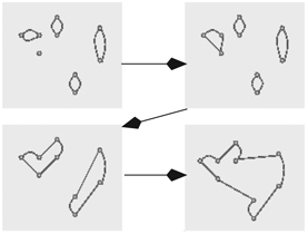
FIGURE 8.15 Neighborhood Tour Heuristic
In general, problem solving involves these steps:
- Precisely define the problem, task, or goal.
- Consider different ways to tackle the problem, perform the task, or achieve the goal. Take into account the effectiveness, efficiency, and degree of complexity of the solution method.
- Attempt to automate the solution by specifying it in an algorithmic form. This can make the solution more foolproof if not completely automatic.
While concepts and ideas in this chapter can help make you a better problem solver, don’t forget to search the Web for answers before inventing a solution of your own.
Exercises
- 8.1 Solve the Magic Tray puzzle in Section 8.1.3. Hint: The configuration shown in Figure 8.3 is one step away from being done.
- 8.2 Consider the Magic Tray puzzle in Section 8.1.3. If we reach into two random pockets at each step, what is the chance of missing a particular pocket after n steps?
- 8.3 Refer to the improved bubblesort algorithm in Section 8.2.2. Show that the variable go_on is true at the end of a pass if and only if no call to exchange is made for any i > 0 in the pass.
- 8.4 Consider the Eight Queens problem. Having positioned 7 queens, we are now trying to place the last queen. Is it true that there can be at most one valid position for the last queen? Why or why not?
- 8.5 Choice of the partition element (pe) is critical to the efficiency of quicksort. A strategy that works well in practice is to pick the first, middle, and last elements, and then choose the median value as the pe. Refine the partition function to implement this improvement (Section 8.3.1).
- 8.6 With your own words, explain the difference between an algorithm and a heuristic.
- 8.7 Study the Tower of Hanoi (Section 8.5) example and explain the power of recursion in your own way.
- 8.8 Computize: What are your own ideas about having a solution vs. having an algorithmic solution to a problem? Please explain at length.
- 8.9 Computize: Give two examples, not found in this book, of problems with a recursive solution.
- 8.10 Computize: Give examples of things with a recursive nature everywhere.
- 8.11 Computize: Estimate the height of the pile you get if you fold a piece of paper in half repeatedly 32 times.
- 8.12 Group discussion topic: My understanding of recursion.
- 8.13 Group discussion topic: Thinking outside the box.
- 8.14 Group discussion topic: Solution by brute force.
Footnote
1 The pe is often also known as the pivot element.