
CHAPTER 13
THE DATA WAREHOUSE
Traditionally, most data was created to support applications that involved current corporate operations: accounting, inventory management, personnel management, and so forth. As people began to understand to power of information systems and their use became more pervasive, other options regarding data began to develop. For example, companies began to perform sales trend analyses that required historic sales data. The idea was to predict future sales and inventory requirements based on past sales history. Applications such as this led to the realization that there is a great deal of value in historic data, and that it would be worthwhile to organize it on a very broad basis. This is the data warehouse.
OBJECTIVES
- Compare the data needs of transaction processing systems with those of decision support systems.
- Describe the data warehouse concept and list its main features.
- Compare the enterprise data warehouse with the data mart.
- Design a data warehouse.
- Build a data warehouse, including the steps of data extraction, data cleaning, data transformation, and data loading.
- Describe how to use a data warehouse with online analytic processing and data mining.
- List the types of expertise needed to administer a data warehouse.
- List the challenges in data warehousing.
CHAPTER OUTLINE
Introduction
The Data Warehouse Concept
- The Data is Subject Oriented
- The Data is Integrated
- The Data is Non-Volatile
- The Data is Time Variant
- The Data Must Be High Quality
- The Data May Be Aggregated
- The Data is Often Denormalized
- The Data is Not Necessarily Absolutely Current
Types of Data Warehouses
Designing a Data Warehouse
- Introduction
- General Hardware Co. Data Warehouse
- Good Reading Bookstores Data Warehouse
- Lucky Rent-A-Car Data Warehouse
- What About a World Music Association Data Warehouse?
Building a Data Warehouse
- Introduction
- Data Extraction
- Data Cleaning
- Data Transformation
- Data Loading
Using a Data Warehouse
- On-Line Analytic Processing
- Data Mining
Administering a Data Warehouse
Challenges in Data Warehousing
Summary
INTRODUCTION
Generally, when we think about information systems, we think about what are known as operational or “ transaction processing systems” (TPS). These are the everyday application systems that support banking and insurance operations, manage the parts inventory on manufacturing assembly lines, keep track of airline and hotel reservations, support Web-based sales, and so on. These are the kinds of application systems that most people quickly associate with the information systems field and, indeed, these are the kinds of application systems that we have used as examples in this book. The databases that support these application systems must have several things in common, which we ordinarily take for granted. They must have up-to-the-moment current data, they must be capable of providing direct access and very rapid response, and they must be designed for sharing by large numbers of users.
But the business world has other needs of a very different nature. These needs generally involve management decision making and typically require analyzing data that has been accumulated over some period of time. They often don't even require the latest, up-to-the-second data! An example occurs in the retail store business, when management has to decide how much stock of particular items they should carry in their stores during the October-December period this year. Management is going to want to check the sales volume for those items during the same three-month period in each of the last five years. If airline management is considering adding additional flights between two cities (or dropping existing flights), they are going to want to analyze lots of accumulated data about the volume of passenger traffic in their existing flights between those two cities. If a company is considering expanding its operations into a new geographical region, management will want to study the demographics of the region's population and the amount of competition it will have from other companies, very possibly using data that it doesn't currently have but must acquire from outside sources.
In response to such management decision-making needs, there is another class of application systems, known as “decision support systems” (DSS), that are specifically designed to aid managers in these tasks. The issue for us in this book about database management is: what kind of database is needed to support a DSS? In the past, files were developed to support individual applications that we would now classify as DSS applications. For example, the five-year sales trend analysis for retail stores described above has been a fairly standard application for a long time and was always supported by files developed for it alone. But, as DSS activity has mushroomed, along with the rest of information systems, having separate files for each DSS application is wasteful, expensive and inefficient, for several reasons:
- Different DSS applications often need the same data, causing duplicate files to be created for each application. As with any set of redundant files, they are wasteful of storage space and update time, and they create the potential for data integrity problems (although, as we will see a little later, data redundancy in dealing with largely historical data is not as great a concern as it is with transactional data).
- While particular files support particular DSS applications, they tend to be inflexible and do not support closely related applications that require slightly different data.
- Individual files tied to specific DSS applications do nothing to encourage other people and groups in the company to use the company's accumulated data to gain a competitive advantage over the competition.
- Even if someone in the company is aware of existing DSS application data that they could use to their own advantage (really, to the company's advantage), getting access to it can be difficult because it is “owned” by the application for which it was created.
When we talked about the advantages of data sharing earlier in this book, the emphasis was on data in transactional systems. But the factors listed above regarding data for decision support systems, which in their own way largely parallel the arguments for shared transactional databases, inevitably led to the concept of broad-based, shared databases for decision support. These DSS databases have come to be known as “data warehouses.” In this chapter, we will discuss the nature, design, and implementation of data warehouses. Later in the chapter we will briefly touch upon some of their key uses.
CONCEPTS IN ACTION
13-A SMITH & NEPHEW
Smith & Nephew is a leader in the manufacture and marketing of medical devices. Headquartered in London, UK, the company has over 7,000 employees and operations in 34 countries. Smith & Nephew focuses on three areas of medical device technology, each run by a separate business unit. In orthopedics, Smith & Nephew is a leading manufacturer of knee, hip, and shoulder replacement joints, as well as products that aid in the repair of broken bones. In endoscopy, the company is the world leader in arthroscopic surgery devices for minimally invasive surgery of the knee and other joints. Last, the company is the world leader in providing products and techniques for advanced wound management. All of this from a beginning in 1856 when Thomas J. Smith opened a pharmaceutical chemist shop in Hull, England. And, yes, he later brought his nephew into the company.
Smith and Nephew supports its orthopedics products business with a state-of-the-art data warehouse. This data warehouse incorporates daily sales and inventory data from its operational SAP system plus global data and data from external sources regarding finance and market data. It provides a decision support environment for sales administrators who must manage and realign sales territories, marketing specialists who must analyze market potentials, product managers, and logistics managers. The data warehouse also supports an executive information system for reporting the company's results to the Orthopedic Executive Staff.

Photo Courtesy of Smith & Nephew
The data warehouse is built on the Oracle RDBMS and runs on Hewlett-Packard Unix hardware. Queries are generated through Oracle query products as well as native SQL. Smith & Nephew's data warehouse architecture employs the classic star schema design, with several major subject areas. These and their fact tables include U.S. sales, global sales, budget, and inventory. The dimension tables, for example for global sales, include customer, time, and product. This arrangement allows historical sales data to be compiled by customer, sales territory, time period, product, and so forth.
THE DATA WAREHOUSE CONCEPT
Informally, a data warehouse is a broad-based, shared database for management decision making that contains data gathered over time. Imagine that at the end of every week or month, you take all the company's sales data for that period and you append it to (add it to the end of) all of the accumulated sales data that is already in the data warehouse. Keep on doing this and eventually you will have several years of company sales data that you can search and query and perform all sorts of calculations on.
More formally and in more detail, the classic definition of a data warehouse is that it is “a subject oriented, integrated, non-volatile, and time variant collection of data in support of management's decisions.”1 In addition, the data in the warehouse must be high quality, may be aggregated, is often denormalized, and is not necessarily absolutely current, Figure 13.1. Let's take a look at each of these data warehouse characteristics.
The Data is Subject Oriented
The data in transactional databases tends to be organized according to the company's TPS applications. In a bank this might mean the applications that handle the processing of accounts; in a manufacturing company it might include the applications that communicate with suppliers to maintain the necessary raw materials and parts on the assembly line; in an airline it might involve the applications that support the reservations process. Data warehouses are organized around “subjects,” really the major entities of concern in the business environment. Thus, subjects may include sales, customers, orders, claims, accounts, employees, and other entities that are central to the particular company's business.
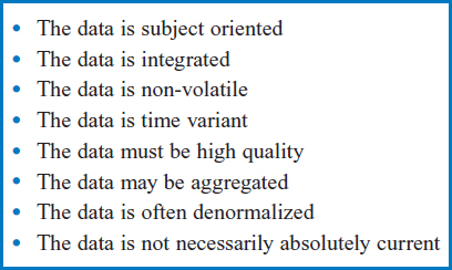
FIGURE 13.1 Characteristics of data warehouse data
The Data is Integrated
Data about each of the subjects in the data warehouse is typically collected from several of the company's transactional databases, each of which supports one or more applications having something to do with the particular subject. Some of the data, such as additional demographic data about the company's customers, may be acquired from outside sources. All of the data about a subject must be organized or “integrated” in such a way as to provide a unified overall picture of all the important details about the subject over time. Furthermore, while being integrated, the data may have to be “transformed.” For example, one application's database tables may measure the company's finished products in centimeters while another may measure them in inches. One may identify countries of the world by name while another may identify them by a numeric code. One may store customer numbers as an integer field while another may store them as a character field. In all of these and in a wide variety of other such cases, the data from these disparate application databases must be transformed into common measurements, codes, data types, and so forth, as they are integrated into the data warehouse.
The Data is Non-Volatile
Transactional data is normally updated on a regular, even frequent basis. Bank balances, raw materials inventories, airline reservations data are all updated as the balances, inventories, and number of seats remaining respectively change in the normal course of daily business. We describe this data as “volatile,” subject to constant change. The data in the data warehouse is non-volatile. Once data is added to the data warehouse, it doesn't change. The sales data for October 2010 is whatever it was. It was totaled up, added to the data warehouse at the end of October 2010, and that's that. It will never change. Changing it would be like going back and rewriting history. The only way in which the data in the data warehouse is updated is when data for the latest time period, the time period just ended, is appended to the existing data.
The Data is Time Variant
Most transactional data is, simply, “current.” A bank balance, an amount of raw materials inventory, the number of seats left on a flight are all the current, up-to-the-moment figures. If someone wants to make a withdrawal from his bank account, the bank doesn't care what the balance was ten days ago or ten hours ago. The bank wants to know what the current balance is. There is no need to associate a date or time with the bank balance; in effect, the data's date and time is always now.(To be sure, some transactional data must include timestamps. A health insurance company may keep six months of claim data online and such data clearly requires timestamps.) On the other hand, data warehouse data, with its historical nature, always includes some kind of a timestamp. If we are storing sales data on a weekly or monthly basis and we have accumulated ten years of such historic data, each weekly or monthly sales figure obviously must be accompanied by a timestamp indicating the week or month (and year!) that it represents.
The Data Must Be High Quality
Transactional data can actually be somewhat forgiving of at least certain kinds of errors. In the bank record example, the account balance must be accurate but if there is, say, a one-letter misspelling of the street name in the account holder's street address, that probably will not make a difference. It will not affect the account balance and the post office will probably still deliver the account statements to the right house. But what if the customer's street address is actually spelled correctly in other transactional files? Consider a section of a data warehouse in which the subject is ‘customer.’ It is crucial to establish an accurate set of customers for the data warehouse data to be of any use. But with the address misspelling in one transactional file, when the data from that file is integrated with the data from the other transactional files, there will be some difficulty in reconciling whether the two different addresses are the same and both represent one customer, or whether they actually represent two different customers. This must be investigated and a decision made on whether the records in the different files represent one customer or two different customers. It is in this sense that the data in the data warehouse must be of higher quality than the data in the transactional files.
The Data May Be Aggregated
When the data is copied and integrated from the transactional files into the data warehouse, it is often aggregated or summarized, for at least three reasons. One is that the type of data that management requires for decision making is generally summarized data. When trying to decide how much stock to order for a store for next December based on the sales data from the last five Decembers, the monthly sales figures are obviously useful but the individual daily sales figures during those last five Decembers probably don't matter much. The second reason for having aggregated data in the data warehouse is that the sheer volume of all of the historical detail data would often make the data warehouse unacceptably huge (they tend to be large as it is!). And the third reason is that if the detail data were stored in the data warehouse, the amount of time needed to summarize the data for management every time a query was posed would often be unacceptable. Having said all that, the decision support environment is so broad that some situations within it do call for detail data and, indeed, some data warehouses do contain at least some detail data.
The Data is Often Denormalized
One of the fundamental truths about database we have already encountered is that data redundancy improves the performance of read-only queries but takes up more disk space, requires more time to update, and introduces possible data integrity problems when the data has to be updated. But in the case of the data warehouse, we have already established that the data is non-volatile. The existing data in the data warehouse never has to be updated. That makes the data warehouse a horse (or a database) of a different color! If the company is willing to tolerate the substantial additional space taken up by the redundant data, it can gain the advantage of the improved query performance that redundancy provides without paying the penalties of increased update time and potential data integrity problems because the existing data is historical and never has to be updated!
The Data is Not Necessarily Absolutely Current
This is really a consequence of the kind of typical time schedule for loading new data into the data warehouse and was implied in “The Data is Time Variant” item above. Say that you load the week-just-ended sales data into the data warehouse every Friday. The following Wednesday, a manager queries the data warehouse for help in making a decision. The data in the data warehouse is not “current” in the sense that sales data from last Saturday through today, Wednesday, is not included in the data warehouse. The question is, does this matter? The answer is, probably not! For example, the manager may have been performing a five-year sales trend analysis. When you're looking at the last five years of data, including or omitting the last five days of data will probably not make a difference.
TYPES OF DATA WAREHOUSES
Thus far, we have been using the term “data warehouse” in a generic sense. But, while there are some further variations and refinements, there are basically two kinds of data warehouses. One is called an enterprise data warehouse (EDW), the other is called a data mart (DM), Figure 13.2. They are distinguished by two factors: their size and the portion of the company that they service (which tend to go hand in hand), and the manner in which they are created and new data is appended (which are also related).
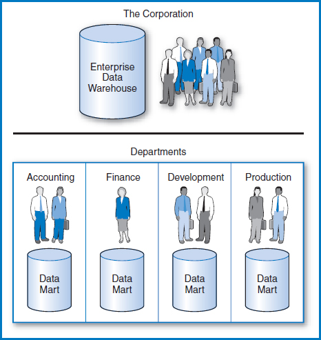
FIGURE 13.2 The enterprise data warehouse and data marts
The Enterprise Data Warehouse (EDW)
The enterprise data warehouse is a large-scale data warehouse that incorporates the data of an entire company or of a major division, site, or activity of a company. Both Smith & Nephew and Hilton Hotels employ such large-scale data warehouses. Depending on its nature, the data in the EDW is drawn from a variety of the company's transactional databases as well as from externally acquired data, requiring a major data integration effort. In data warehouse terminology, a full-scale EDW is built around several different subjects. The large mass of integrated data in the EDW is designed to support a wide variety of DSS applications and to serve as a data resource with which company managers can explore new ways of using the company's data to its advantage. Many EDWs restrict the degree of denormalization because of the sheer volumes of data that large-scale denormalization would produce.
The Data Mart (DM)
A data mart is a small-scale data warehouse that is designed to support a small part of an organization, say a department or a related group of departments. As we saw, Hilton Hotels copies data from its data warehouse into a data mart for marketing query purposes. A company will often have several DMs. DMs are based on a limited number of subjects (possibly one) and are constructed from a limited number of transactional databases. They focus on the business of a department or group of departments and thus tend to support a limited number and scope of DSS applications. Because of the DM's smaller initial size, there is more freedom to denormalize the data. Managerially, the department manager may feel that she has more control with a local DM and a greater ability to customize it to the department's needs.
Which to Choose: The EDW, the DM, or Both?
Should a company have an EDW, multiple DMs, or both? This is the kind of decision that might result from careful planning, or it might simply evolve as a matter of management style or even just happenstance. Certainly, there are companies that have very deliberately and with careful planning decided to invest in developing an EDW. There are also companies that have made a conscious decision to develop a series of DMs instead of an EDW. In other situations, there was no careful planning, at all. There have been situations in managerially decentralized companies in which individual managers decided to develop DMs in their own departments. At times DMs have evolved from the interests of technical people in user departments.
In companies that have both an EDW and DMs, there are the questions of “Which came first?” and “Were they developed independently or derived from each other?” This can go either way. In regard to data warehousing, the term, “top-down development” implies that the EDW was created first and then later data was extracted from an EDW to create one or more DMs, initially and on an ongoing basis. Assuming that the company has made the decision to invest in an EDW, this can make a great deal of sense. For example, once the data has been scrutinized and its quality improved (see “data cleaning” below) as it was entered into the EDW, downloading portions of it to DMs retains the high quality without putting the burden for this effort on the department developing the DM. Development in the other direction is possible, too. A company that has deliberately or as a matter of circumstance developed a series of independent DMs may decide, in a “bottom-up development” fashion, to build an EDW out of the existing DMs. Clearly, this would have to involve a round of integration and transformation beyond those that took place in creating the individual DMs.
DESIGNING A DATA WAREHOUSE
Introduction
As data warehousing has become a broad topic with many variations in use, it comes as no surprise that there are a variety of ways to design data warehouses. Two of the characteristics of data warehouses are central to any such design: the subject orientation and the historic nature of the data. That is, the data warehouse (or each major part of the data warehouse) will be built around a subject and have a temporal (time) component to it. Data warehouses are often called multidimensional databases because each occurrence of the subject is referenced by an occurrence of each of several dimensions or characteristics of the subject, one of which is time. For example, in a hospital patient tracking and billing system, the subject might be charges and dimensions might include patient, date, procedure, and doctor. When there are just two dimensions, for example the charges for a particular patient on a particular date, they can easily be visualized on a flat piece of paper, Figure 13.3. When there are three dimensions, for example the charges for a particular procedure performed on a particular patient on a particular date, they can be represented as a cube and still drawn on paper, Figure 13.4. When there are four (or more) dimensions, say the charges for a particular procedure ordered by a particular doctor performed on a particular patient on a particular date, it takes some imagination (although there are techniques for combining dimensions that bring the visual representation back down to two or three dimensions). There are data warehouse products on the market that have special-purpose data structures to store such multidimensional data. But there is also much interest in storing such data in relational databases. A way to store multidimensional data in a relational database structure is with a model known as the star schema. The name comes from the visual design in which the subject is in the middle and the dimensions radiate outwards like the rays of a star. As noted earlier, Smith & Nephew employs the star schema design for its data warehouse, as does Hilton Hotels for at least part of its data warehouse environment.
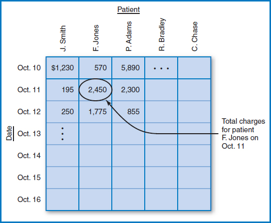
FIGURE 13.3 Hospital patient tracking and billing system data with two dimensions
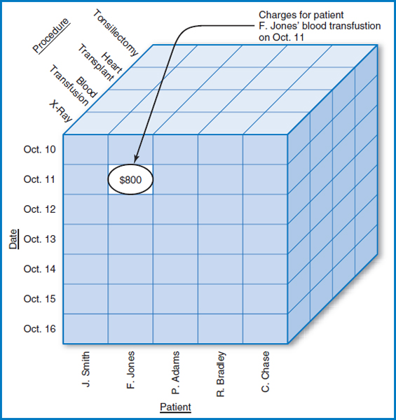
FIGURE 13.4 Hospital patient tracking and billing system data with three dimensions
General Hardware Co. Data Warehouse
Figure 13.5 repeats the General Hardware relational database and Figure 13.6 shows a star schema for the General Hardware Co., with SALE as the subject. Star schemas have a “fact table,” which represents the data warehouse “subject,” and several “dimension tables.” In Figure 13.6, SALE is the fact table and SALESPERSON, PRODUCT, and TIME PERIOD are the dimension tables. The dimension tables will let the data in the fact table be studied from many different points of view. Notice that there is a one-to-many relationship between each dimension table entity and the fact table entity. Furthermore, the “one side” of the relationship is always the dimension table and the ' “many side” of the relationship is always the fact table. For a particular salesperson there are many sales records, but each sales record is associated with only one salesperson. The same is true of products and time periods.
To begin to understand this concept and see it come to life, refer back to the SALES table in Figure 13.5, in which General Hardware keeps track of how many units of each product each salesperson has sold in the most recent time period, say in the last week. But what if we want to record and keep track of the sales for the most recent week, and the week before that, and the week before that, and so on going back perhaps five or ten years? That is a description of a data warehouse. The SALE table in the star schema of Figure 13.6 also reflects General Hardware's sales by salesperson and product but with a new element added: time. This table records the quantity of each product that each salesperson sold in each time period stored.
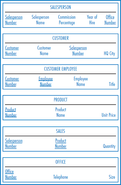
FIGURE 13.5 The General Hardware Company relational database
The SALE table in Figure 13.6 has to have a primary key, like any relational table. As shown in the figure, its primary key is the combination of the Salesperson Number, Product Number, and Time Period Number attributes. But each of those attributes also serves as a foreign key. Each one leads to one of the dimension tables, as shown in Figure 13.6. Some historic data can be obtained from the fact table alone. Using the SALE table, alone, for example, we could find the total number of units of a particular product that a particular salesperson has sold for as long as the historical sales records have been kept, assuming we know both the product's product number and the salesperson's salesperson number. We would simply add the Quantity values in all of the SALE records for that salesperson and product. But the dimension tables provide, well, a whole new dimension! For example, focusing in on the TIME PERIOD's Year attribute and taking advantage of this table's foreign key connection to the SALE table, we could refine the search to find the total number of units of a particular product that a particular salesperson sold in a particular single year or in a particular range of years. Or, focusing on the PRODUCT table's Unit Price attribute and the TIME PERIOD table's Year attribute, we could find the total number of units of expensive (unit price greater than some amount) products that each salesperson sold in a particular year. To make this even more concrete, suppose that we want to decide which of our salespersons who currently are compensated at the 10% commission level should receive an award based on their sales of expensive products over the last three years. We could sum the quantity values of the SALE table records by grouping them based on an attribute value of 10 in the Commission Percentage attribute of the SALESPERSON table, an attribute value greater than 50 (dollars) in the Unit Price attribute of the PRODUCT table, and a Year attribute representing each of the last three years in the TIME PERIOD table. The different combinations and possibilities are almost endless.
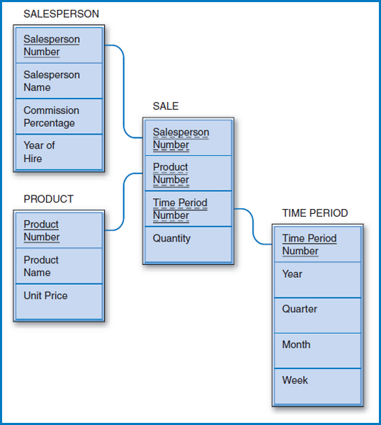
FIGURE 13.6 General Hardware Company data warehouse star schema design
Figure 13.7 shows some sample data for General Hardware's star schema data warehouse. The fact table, SALE, is on the left and the three dimension tables are on the right. The rows shown in the SALE table are numbered on the left just for convenience in discussion. Look at the TIME PERIOD table in Figure 13.7. First of all, it is clear from the TIME PERIOD table that a decision was made to store data by the week and not by any smaller unit, such as the day. In this case, even if the data in the transactional database is being accumulated daily, it will be aggregated into weekly data in the data warehouse. Notice that the data warehouse began in the first week of the first month of the first quarter of 1997 and that this week was given the Time Period Number value of 001. The week after that was given the Time Period Number value of 002, and so on to the latest week stored. Now, look at the SALE table. Row 10 indicates that salesperson 137 sold 59 units of product 24013 during time period 103, which according to the TIME PERIOD table was the second week of the third month of the fourth quarter of 1998 (i.e. the second week of December, 1998). Row 17 of the SALE table shows that salesperson 204 sold 44 units of product 16386 during time period 331, which was the third week of May, 2003. Overall, as you look at the SALE table from row 1 down to row 20, you can see the historic nature of the data and the steady, forward time progression as the Time Period Number attribute starts with time period 001 in the first couple of records and steadily increases to time period 331 in the last batch of records.
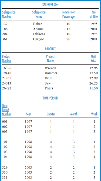
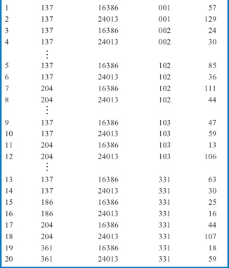
FIGURE 13.7 General Hardware Company data warehouse sample data
Good Reading Bookstores Data Warehouse
Does Good Reading Bookstores need a data warehouse? Actually, this is a very good question, the answer to which is going to demonstrate a couple of important points about data warehouses. At first glance, the answer to the question seems to be: maybe not! After all, the sales data in Good Reading's transactional database already carries a date attribute, as shown in the SALE table of Figure 5.16. Thus, it looks like Good Reading's transactional database is already historical! But Good Reading does need a data warehouse for two reasons. One is that, while Good Reading's transactional database performs acceptably with perhaps the last couple of months of data in it, its performance would become unacceptable if we tried to keep ten years of data in it. The other reason is that the kinds of management decision making that require long-term historical sales data do not require daily data. Data aggregated to the week level is just fine for Good Reading's decision making purposes and storing the data on a weekly basis saves a lot of time over retrieving and adding up much more data to answer every query on data stored at the day level.
Figure 13.8 shows the Good Reading Bookstores data warehouse star schema design. The fact table is SALE and each of its records indicates how many of a particular book a particular customer bought in a particular week (here again week is the lowest-level time period) and the price that the customer paid per book. For this to make sense, there must be a company rule that the price of a book cannot change in the middle of a week, since each SALE table row has space to store only one price to go with the total quantity of that book purchased by that customer during that week. The design in Figure 13.8 also has a feature that makes it a “snowflake” design: one of the dimension tables, BOOK, leads to yet another dimension table, PUBLISHER. Consistent with the rest of the star schema, the snowflake relationship is one-to-many, “inward” towards the center of the star. A publisher publishes many books but a book is associated with only one publisher.
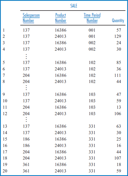
FIGURE 13.8 Good Reading Bookstores data warehouse star schema design with snowflake feature
To help in deciding how many copies of Moby Dick to order for its stores in Florida during the upcoming Christmas season, Good Reading could check how many copies of Moby Dick were purchased in Florida during each of the last five Decembers. This query would require the Book Name attribute of the BOOK table, the State and Country attributes of the CUSTOMER table, and the Year and Month attributes of the TIME PERIOD table. To help in deciding whether to open more stores in Dallas, TX, Good Reading could sum the total number of all books purchased in all their existing Dallas stores during each of the last five years. The snowflake feature expands the range of query possibilities even further. Using the Country attribute of the PUBLISHER table, the State and Country attributes of the CUSTOMER table, and the Quarter and Year attributes of the TIME PERIOD table, they could find the total number of books published in Brazil that were purchased by customers in California during the second quarter of 2009.
Lucky Rent-A-Car Data Warehouse
Like Good Reading Bookstores' transactional database, Lucky Rent-A-Car's transactional database (Figure 5.18) already carries a date attribute (two, in fact) in its RENTAL table. The reasoning for creating a data warehouse for Lucky is based on the same argument that we examined for Good Reading, that its transactional database would bog down under the weight of all the data if we tried to store ten years or more of rental history data in it. Interestingly, in the Lucky case, the data warehouse should still store the data down to the day level (resulting in a huge data warehouse). Why? In the rental car business, it is important to be able to check historically whether, for example, more cars were rented on Saturdays over a given time period than on Tuesdays.
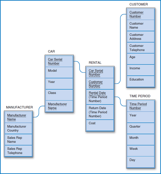
Figure 13.9 shows the Lucky Rent-A-Car data warehouse star schema design. The fact table is RENTAL. In this case, as implied above, the fact table does not contain aggregated data. Every car rental transaction is recorded for posterity in the data warehouse. Notice that this data warehouse has a snowflake feature since the CAR dimension table is connected outwards to the MANUFACTURER table. The query possibilities in this data warehouse are very rich. Lucky could ask how many mid-size (the CAR table's Class attribute) General Motors cars were rented on July weekends in each of the last five years. To find who some of their most valuable customers are for marketing purposes, Lucky could identify the customers (and create a name and address list for them) who rented full-size cars at least three times for at least a week each time during the winter months of each of the last three years. Or, using the Manufacturer Country attribute of the MANUFACTURER table in the snowflake, they could find the amount of revenue (based on the RENTAL table's Cost attribute) that they generated by renting Japanese cars during the summer vacation period in each of the last eight years.
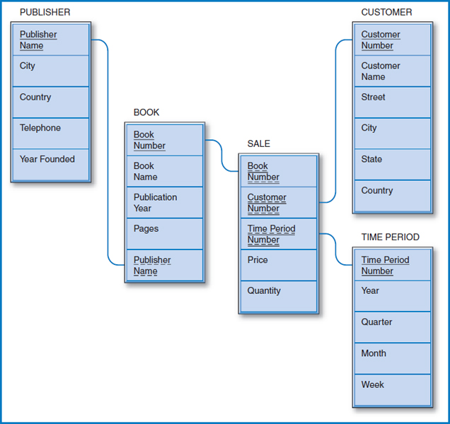
FIGURE 13.9 Lucky Rent-A-Car data warehouse star schema design with snowflake feature
What About a World Music Association Data Warehouse?
Did you notice that we haven't talked about a data warehouse for the World Music Association (WMA), whose transactional database is shown in Figure 5.17? If there were to be such a data warehouse, its most likely subject would be RECORDING, as the essence of WMA's business is to keep track of different recordings made of different compositions by various orchestras. There is already a Year attribute in the RECORDING table of Figure 5.17. In this sense, the main data of the World Music Association's transactional database is already “timestamped,” just like Good Reading Bookstores' and Lucky Rent-A-Car's data. We gave reasons for creating data warehouses for Good Reading and for Lucky, so what about WMA? First, the essence of the WMA data is historical. We might be just as interested in a recording made fifty years ago as one made last year. Second, by its nature, the amount of data in a WMA-type transactional database is much smaller than the amount of data in a Good Reading or Lucky-type transactional database. The latter two transactional databases contain daily sales records in high-volume businesses. Even on a worldwide basis, the number of recordings orchestras make is much smaller in comparison. So, the conclusion is that, since the nature of the WMA transactional database blurs with what a WMA data warehouse would look like and the amount of (historical) data in the WMA transactional database is manageable, there is no need for a WMA data warehouse.
YOUR TURN
13.1 DESIGNING A UNIVERSITY DATA WAREHOUSE
Universities create a great deal of data. There is data about students, data about professors, data about courses, data about administrative units such as academic department, data about the physical plant, and accounting data, just as in any business operation. Some of the data is current, such as the students enrolled in particular courses in the current semester. But it may be useful to maintain some of the data on a historical basis.
QUESTION:
Think about what data a university might want to maintain on a historical basis. Design a data warehouse for this historical data. You may focus on students as the subject of the data warehouse or any other entity that you wish.
BUILDING A DATA WAREHOUSE
Introduction
Once the data warehouse has been designed, there are four steps in actually building it. As shown in Figure 13.10, these are:
- Data Extraction
- Data Cleaning
- Data Transformation
- Data Loading
Let's take a look at each of these steps.
Data Extraction
Data extraction is the process of copying data from the transactional databases in preparation for loading it into the data warehouse. There are several important points to remember about this. One is that it is not a one-time event. Obviously, there must be an initial extraction of data from the transactional databases when the data warehouse is first built, but after that it will be an ongoing process, performed at regular intervals, perhaps daily, weekly, or monthly, when the latest day's, week's, or month's transactional data is added to the data warehouse. Another point is that the data is likely to come from several transactional databases. Specific data (that means not necessarily all of the data) in each transactional database is copied and merged to form the data warehouse. There are pitfalls along the way that must be dealt with, such as, for example, that the employee serial number attribute may be called, “Employee Number” in one transactional database and “Serial Number” in another. Or, looking at it another way, the attribute name “Serial Number” may mean “Employee Serial Number” in one database and “Finished Goods Serial Number” in another.
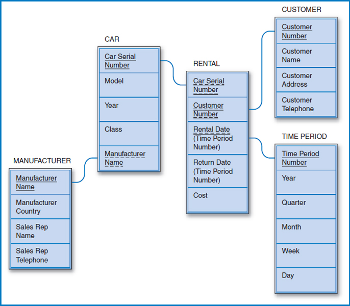
FIGURE 13.10 The four steps in building a data warehouse
Some of the data entering into this process may come from outside of the company. For example, there are companies whose business is to sell demographic data about people to companies that want to use it for marketing purposes. This process is known as data enrichment. Figure 13.11 shows enrichment data added to Lucky Rent-A-Car's data warehouse CUSTOMER dimension table from Figure 13.9. Notice that in the data enrichment process, age, income, and education data are added, presumably from some outside data source. Lucky might use this data to try to market the rental of particular kinds of cars to customers who fall into certain demographic categories. We will talk more about this later in the section on data mining.
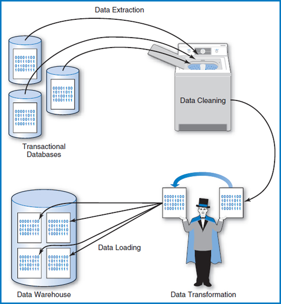
FIGURE 13.11 Lucky Rent-A-Car data warehouse design with enrichment data added to the CUSTOMER table
Data Cleaning
Transactional data can contain all kinds of errors that may or may not affect the applications that use it. For example, if a customer's name is misspelled but the Post Office can correctly figure out to whom to deliver something, no one may ever bother to fix the error in the company's customer table. On the other hand, if a billing amount is much too high, the assumption is that the customer will notice it and demand that it be corrected. Data warehouses are very sensitive to data errors and as many such errors as possible must be “cleaned” (the process is also referred to as “cleansed” or “scrubbed”) as the data is loaded into the data warehouse. The point is that if data errors make it into the data warehouse, they can throw off the totals and statistics generated by the queries that are designed to support management decision making, compromising the value of the data warehouse.
There are two steps to cleaning transactional data in preparation for loading it into a data warehouse. The first step is to identify the problem data and the second step is to fix it. Identifying the problem data is generally a job for a program, since having people scrutinize the large volumes of data typical today would simply take too long. Fixing the identified problems can be handled by sophisticated artificial intelligence programs or by creating exception reports for employees to scrutinize. Figure 13.12 shows sample data from two of Good Reading Bookstores' transactional database tables (see Figure 5.16). (The row numbers on the left are solely for reference purposes in this discussion.) Each table has several errors that would have to be corrected as the data is copied, integrated, and aggregated into a data warehouse. Some of the errors shown may be less likely than others actually to turn up in today's more sophisticated application environment, but as a group they make the point that there are lots of potential data hazards out there.
There are four errors or possible errors in the CUSTOMER table, Figure 13.12a:
- Missing Data: In row 1, the City attribute is blank. It's possible that a program could check an online “white pages” listing of Tennessee (State=“TN” in row 1), look for a Mervis at 123 Oak St., and in that way discover the city and automatically insert it as the City value in row 1. But it should also be clear that this type of error could occur in data for which there is no online source of data for cross checking. In that case, the error may have to be printed in an error report for an employee to look at.
- Questionable Data: Rows 2 and 6, each of which has a different customer number, both involve customers named Gomez who live at 345 Main Ave., Columbus, USA. But one city is Columbus, Ohio (“OH”) and the other is Columbus, Georgia (“GA”), each of which is a valid city/state combination. So the question is whether these are really two different people who happen to have the same name and street address in two different cities named Columbus, or whether they are the same person (if so, one of the state designations is wrong and there should only be one customer number).
FIGURE 13.12 Good Reading Bookstores sample data prior to data cleaning
- Possible Misspelling: Rows 3 and 8 have different customer numbers but are otherwise identical except for a one-letter difference in the customer name, “Taylor” vs. “Tailor.” Do both rows refer to the same person? For the sake of argument, say that an online white pages is not available but a real estate listing indicating which addresses are single-family houses and which are apartment buildings is. A program could be designed to assume that if the address is a single-family house, there is a misspelling and the two records refer to the same person. On the other hand, if the address is an apartment building, they may, indeed, be two different people.
- Impossible Data: Row 10 has a state value of “RP.” There is no such state abbreviation in the U.S. This must be flagged and corrected either automatically or manually.
There are also four errors or possible errors in the SALE table in Figure 13.12b. The data in this table is more numeric in nature than the CUSTOMER table data:
- Questionable Data: In row 2, the quantity of a particular book purchased in a single transaction is 21. This is possible, but generally unlikely. A program may be designed to decide whether to leave it alone or to report it as an exception depending on whether the type of book it is makes it more or less likely that the quantity is legitimate.
- Impossible/Out-of-Range Data: Row 5 indicates that a single book cost $3,200.99. This is out of the possible range for book prices and must either be corrected, if the system knows the correct price for that book (based on the book number), or reported as an exception.
- Apparently Incorrect Data: The Customer Number in row 8 is invalid. We don't have a customer with customer number 12738. But we do have a customer with customer number 12739 (see row 6 of the CUSTOMER table in part a of the figure). A person would have to look into this one.
- Impossible Data: Row 10 shows a negative price for a book, which is impossible.
Data Transformation
As the data is extracted from the transactional databases, it must go through several kinds of transformations on its way to the data warehouse:
- We have already talked about the concept of merging data from different transactional databases to form the data warehouse tables. This is indeed one of the major data transformation steps.
- In many cases the data will be aggregated as it is being extracted from the transactional databases and prepared for the data warehouse. Daily transactional data may be summed to form weekly or monthly data as the lowest level of data storage in the data warehouse.
- Units of measure used for attributes in different transactional databases must be reconciled as they are merged into common data warehouse tables. This is especially common if one transactional database uses the metric system and another uses the English system. Miles and kilometers, pounds and kilograms, gallons and liters all have to go through a conversion process in order to wind up in a unified way in the data warehouse.
- Coding schemes used for attributes in different transactional databases must be reconciled as they are merged into common data warehouse tables. For example, states of the U.S. could be represented in different databases by their full names, two-letter postal abbreviations, or a numeric code from 1 to 50. Countries of the world could be represented by their full names, standard abbreviations used on vehicles, or a numeric code. Another major issue along these lines is the different ways that dates can be stored.
- Sometimes values from different attributes in transactional databases are combined into a single attribute in the data warehouse or the opposite occurs: a multipart attribute is split apart. Consider the first name and last name of employees or customers as an example of this.
Data Loading
Finally, after all of the extracting, cleaning, and transforming, the data is ready to be loaded into the data warehouse. We would only repeat here that after the initial load, a schedule for regularly updating the data warehouse must be put in place, whether it is done on a daily, weekly, monthly, or some other designated time period basis. Remember, too, that data marts that use the data warehouse as their source of data must also be scheduled for regular updates.
USING A DATA WAREHOUSE
We have said that the purpose of a data warehouse is to support management decision-making. Indeed, such “decision support” and the tools of its trade are major topics by themselves and not something we want to go into in great detail here. Still, it would be unsatisfying to leave the topic of data warehouses without considering at all how they are used. We will briefly discuss two major data warehouse usage areas: on-line analytic processing and data mining.
On-Line Analytic Processing
On-Line Analytic Processing (OLAP) is a decision support methodology based on viewing data in multiple dimensions. Actually, we alluded to this topic earlier in this chapter when we described the two-, three-, and four-dimensional scenarios for recording hospital patient tracking and billing data. There are many OLAP systems on the market today. As we said before, some employ special purpose database structures designed specifically for multidimensional OLAP-type data. Others, known as relational OLAP or “ROLAP” systems, store multidimensional data in relational databases using the star schema design that we have already covered!
How can OLAP data be used? The OLAP environment's multidimensional data is very well suited for querying and for multi-time period trend analyses, as we saw in the star schema discussion. In addition, several other data search concepts are commonly associated with OLAP:
- Drill-Down: This refers to going back to the database and retrieving finer levels of data detail than you have already retrieved. If you begin with monthly aggregated data, you may want to go back and look at the weekly or daily data, if the data warehouse supports it.
- Slice: A slice of multidimensional data is a subset of the data that focuses on a single value of one of the dimensions. Figure 13.13 is a slice of the patient data “cube” of Figure 13.4, in which a single value of the patient attribute, F. Jones, is nailed down and the data in the other dimensions is displayed.
- Pivot or Rotation: While helpful in terms of visualization, this is merely a matter of interchanging the data dimensions, for example interchanging the data on the horizontal and vertical axes in a two-dimensional view.
Data Mining
As huge data warehouses are built and data is increasingly considered a true corporate resource, a natural movement towards squeezing a greater and greater competitive advantage out of the company's data has taken place. This is especially true when it comes to the data warehouse, which, after all, is intended not to support daily operations but to help management improve the company's competitive position in any way it can. Certainly, one major kind of use of the data warehouse is the highly flexible data search and retrieval capability represented by OLAP-type tools and techniques. Another major kind of use involves “data mining.”
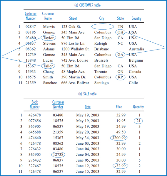
FIGURE 13.13 A ‘slice’ of the hospital patient tracking and billing system data
Data mining is the searching out of hidden knowledge in a company's data that can give the company a competitive advantage in its marketplace. This would be impossible for people to do manually because they would immediately be overwhelmed by the sheer amount of data in the company's data warehouse. It must be done by software. In fact, very sophisticated data mining software has been developed that uses several advanced statistical and artificial intelligence techniques such as:
- Case-based learning
- Decision trees
- Neural networks
- Genetic algorithms
Describing these techniques is beyond the scope of this book. But it's worth taking a quick look at a couple of the possibilities from an application or user's point of view.
One type of data mining application is known as “market basket analysis.” For example, consider the data collected by a supermarket as it checks out its customers by scanning the bar codes on the products they're purchasing. The company might have software study the collected “market baskets,” each of which is literally the goods that a particular customer bought in one trip to the store. The software might try to discover if certain items “fall into” the same market basket more frequently than would otherwise be expected. That last phrase is important because some combinations of items in the same market basket are too obvious or common to be of any value. For example, finding eggs and milk being bought together frequently is not news. On the other hand, a piece of data mining folklore has it that one such study was done and discovered that people who bought disposable diapers also frequently bought beer (you can draw your own conclusions on why this might be the case).The company could use this to advantage by stacking some beer near the diapers in its stores so that when someone comes in to buy diapers, they might make an impulse decision to buy the beer sitting next to it, too. Another use of market basket data is part of the developing marketing discipline of “customer relationship management.” If, through data mining, a supermarket determines that a particular customer who spends a lot of money in the store often buys a particular product, they might offer her discount coupons for that product as a way of rewarding her and developing “customer loyalty” so that she will keep coming back to the store.
Another type of data mining application looks for patterns in the data. Earlier, we suggested that Lucky Rent-A-Car might buy demographic data about its customers to “enrich” the data about them in its data warehouse. Once again, consider Figure 13.11 with its enriched (Age, Income, and Education attributes added) CUSTOMER dimension table. Suppose, and this is quite realistic, that Lucky joined its RENTAL fact table with its CAR and CUSTOMER dimension tables, including only such attributes in the result as would help it identify its most valuable customers, for example those who spend a lot of money renting “luxury” class cars. Figure 13.14 shows the resulting table, with the rows numbered on the left for convenience here. The Class and Manufacturer Name attributes came from the CAR table, the Cost attribute (the revenue for a particular rental transaction) came from the RENTAL table, and the Customer Number, Age, Income, and Education attributes came from the CUSTOMER table. While it would take much more data than this to really find statistically significant data patterns, the sample data in the figure gives a rough idea of what a pattern might look like. Rows 2, 5, 8, and 11 all involve rentals of luxury-class cars with high cost (revenue to the company) figures. As you look across these rows to the customer demographics, you find “clusters” in age, income, and education. These expensive, luxury car rental transactions all involved people in their mid-40s with high income and education levels. On the other hand, rows 10 and 14 involved people who also had high income and education levels. But these people were not in their mid-40s and they did not rent luxury cars and run up as big a bill. With enough such data, Lucky might conclude that it could make more money by heavily promoting its luxury cars to customers in their mid-40s with high income and education levels. If its competitors have not thought of this, then Lucky has gained a competitive advantage by “mining” its data warehouse.
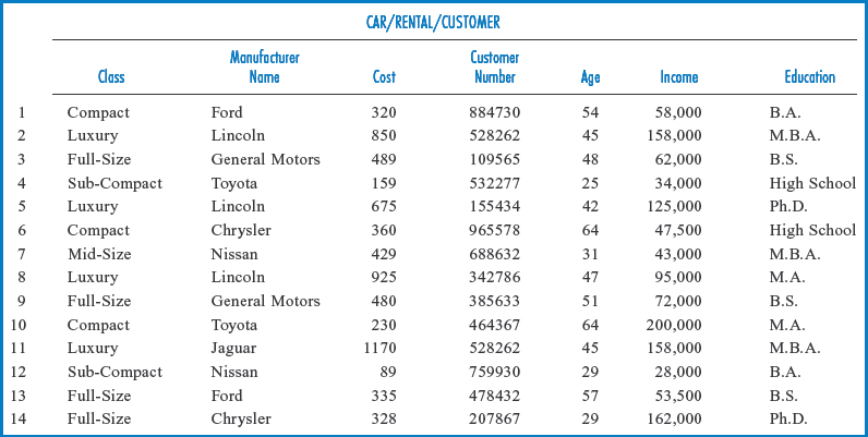
FIGURE 13.14 Lucky Rent-A-Car enriched data, integrated for data mining
YOUR TURN
13.2 USING A UNIVERSITY DATA WAREHOUSE
Consider the university data warehouse that you designed in the Your Turn exercise earlier in this chapter.
QUESTION:
Develop a plan for using your university data warehouse. What benefits can you think of to querying the data warehouse? What kinds of new knowledge might you discover by using data mining techniques on the data warehouse?
ADMINISTERING A DATA WAREHOUSE
In Chapter 10, we discussed the issues of managing corporate data and databases with people called data administrators and database administrators. As a huge database, the data warehouse certainly requires a serious level of management. Further, its unique character requires a strong degree of personnel specialization in its management (some have even given the role its own name of “data warehouse administrator”). In fact, managing the data warehouse requires three kinds of heavily overlapping employee expertise:
- Business Expertise
- An understanding of the company's business processes underlying an understanding of the company's transactional data and databases.
- An understanding of the company's business goals to help in determining what data should be stored in the data warehouse for eventual OLAP and data mining purposes.
- Data Expertise
- An understanding of the company's transactional data and databases for selection and integration into the data warehouse.
- An understanding of the company's transactional data and databases to design and manage data cleaning and data transformation as necessary.
- Familiarity with outside data sources for the acquisition of enrichment data.
- Technical Expertise
- An understanding of data warehouse design principles for the initial design.
- An understanding of OLAP and data mining techniques so that the data warehouse design will properly support these processes.
- An understanding of the company's transactional databases in order to manage or coordinate the regularly scheduled appending of new data to the data warehouse.
- An understanding of handling very large databases in general (as the data warehouse will inevitably be) with their unique requirements for security, backup and recovery, being split across multiple disk devices, and so forth.
The other issue in administering a data warehouse is metadata; i.e., the data warehouse must have a data dictionary to go along with it. The data warehouse is a huge data resource for the company and has great potential to give the company a competitive advantage. But, for this to happen, the company's employees have to understand what data is in it! And for two reasons. One is to think about how to use the data to the company's advantage, through OLAP and data mining. The other is actually to access the data for processing with those techniques.
CHALLENGES IN DATA WAREHOUSING
Data warehousing presents a distinct set of challenges. Many companies have jumped into data warehousing with both feet, only to find that they had bitten off more than they could chew and had to back off. Often, they try again with a more gradual approach and eventually succeed. Many of the pitfalls of data warehousing have already been mentioned at one point or another in this chapter. These include the technical challenges of data cleaning and finding more “dirty” data than expected, problems associated with coordinating the regular appending of new data from the transactional databases to the data warehouse, and difficulties in managing very large databases, which, as we have said, the data warehouse will inevitably be. There is also the separate challenge of building and maintaining the data dictionary and making sure that everyone who needs it understands what's in it and has access to it.
Another major challenge of a different kind is trying to satisfy the user community. In concept, the idea is to build such a broad, general data warehouse that it will satisfy all user demands. In practice, decisions have to be made about what and how much data it is practical to incorporate in the data warehouse at a given time and at a given point in the development of the data warehouse. Unfortunately, it is almost inevitable that some users will not be satisfied in general with the data at their disposal and others will want the data warehouse data to be modified in some way to produce better or different results. And that's not a bad thing! It means that people in the company understand or are gaining an appreciation for the great potential value of the data warehouse and are impatient to have it set up the way that will help them help the company the most—even if that means that the design of the data warehouse and the data in it are perpetually moving targets.
SUMMARY
A data warehouse is a historical database used for applications that require the analysis of data collected over a period of time. A data warehouse is a database whose data is subject oriented, integrated, non-volatile, time variant, high quality, aggregated, possibly denormalized, and not necessarily absolutely current. There are two types of data warehouses: the enterprise data warehouse and the data mart. Some companies maintain one type, some the other, and some both.
Data warehouses are multidimensional databases. They are often designed around the star schema concept. Building a data warehouse is a multi-step process that includes data extraction, data cleaning, data transformation, and data loading. There are several methodologies for using a data warehouse, including on-line analytic processing and data mining. Data warehouses have become so large and so important that it takes special skills to administer them.
KEY TERMS
Aggregated data
Data cleaning
Data enrichment
Data extraction
Data loading
Data mart
Data mining
Data transformation
Data warehouse
Data warehouse administrator
Decision support system (DSS)
Dimension
Drill-down
Enterprise data warehouse
Historic data
Integrated
Market basket analysis
Multidimensional database
Non-volatile
On-line analytic processing (OLAP)
Pivot or rotation
Slice
Snowflake design
Star schema
Subject oriented
Time variant
Transaction processing system
(TPS)
QUESTIONS
- What is the difference between transactional processing systems and decision support systems?
- Decision support applications have been around for many years, typically using captive files that belong to each individual application. What factors led to the movement from this environment towards the data warehouse?
- What is a data warehouse? What is a data warehouse used for?
- Explain each of the following concepts. The data in a data warehouse:
- Is subject oriented.
- Is integrated.
- Is non-volatile.
- Is time variant.
- Must be high quality.
- May be aggregated.
- Is often denormalized.
- Is not necessarily absolutely current.
- What is the difference between an enterprise data warehouse and a data mart?
- Under what circumstances would a company build data marts from an enterprise data warehouse? Build an enterprise data warehouse from data marts?
- What is a multidimensional database?
- What is a star schema? What are fact tables? What are dimension tables?
- What is a snowflake feature in a star schema?
- After a data warehouse is designed, what are the four steps in building it?
- Name and describe three possible problems in transactional data that would require “data cleaning” before the data can be used in a data warehouse.
- Name and describe three kinds of data transformations that might be necessary as transactional data is integrated and copied into a data warehouse.
- What is online analytic processing (OLAP?) What does OLAP have to do with data warehouses?
- What do the following OLAP terms mean?
- Drill-down.
- Slice.
- Pivot or rotation.
- What is data mining? What does data mining have to do with data warehouses?
- Describe the ideal background for an employee who is going to manage the data warehouse.
- Describe the challenges involved in satisfying a data warehouse's user community.
EXERCISES
- Video Centers of Europe, Ltd. data warehouse:
- Design a multidimensional database using a star schema for a data warehouse for the Video Centers of Europe, Ltd. business environment described in the diagram associated with Exercise 2.2. The subject will be “rental,” which represents a particular tape or DVD being rented by a particular customer. As stated in Exercise 2.2, be sure to keep track of the rental date and the price paid. Include a snowflake feature based on the actor, movie, and tape/DVD entities.
- Describe three OLAP uses of this data warehouse.
- Describe one data mining use of this data warehouse.
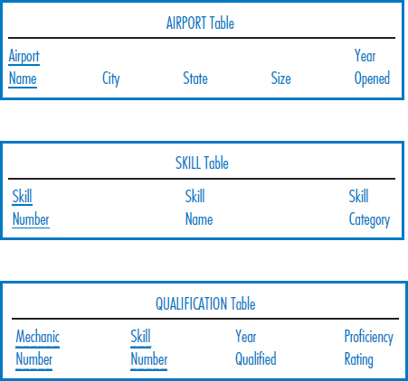
- Best Airlines, Inc., data warehouse:
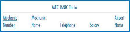
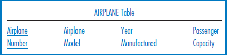
In the exercises in Chapter 8, we saw the following relational database, which Best Airlines uses to keep track of its mechanics, their skills, and their airport locations. Mechanic number, airport name, and skill number are all unique fields. Size is an airport's size in acres. Skill Category is a skill's category, such as an engine skill, wing skill, tire skill, etc. Year Qualified is the year that a mechanic first qualified in a particular skill; Proficiency Rating is the mechanic's proficiency rating in a particular skill. We now add the following tables to the database that record data about airplanes and maintenance performed on them. A maintenance event is a specific maintenance activity performed on an airplane.
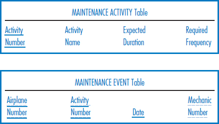
- Design a multidimensional database using a star schema for a data warehouse for the Best Airlines, Inc., airplane maintenance environment described by the complete seven-table relational database above. The subject will be maintenance event. Include snowflake features as appropriate.
- Describe three OLAP uses of this data warehouse.
- Describe one data mining use of this data warehouse
MINICASES
- Happy Cruise Lines data warehouse:
- Design a multidimensional database using a star schema for a data warehouse for the Happy Cruise Lines business environment described in Minicase 2.1. The subject will be “passage,” which represents a particular passenger booking on a particular cruise. As stated in Minicase 2.1, be sure to keep track of the fare that the passenger paid for the cruise and the passenger's satisfaction rating of the cruise.
- Describe three OLAP uses of this data warehouse.
- Describe one data mining use of this data warehouse.
- Super Baseball League data warehouse:
- Design a multidimensional database using a star schema for a data warehouse for the Super Baseball League business environment described in Minicase 2.2. The subject will be “affiliation,” which represents a particular player having played on a particular team. As stated in Minicase 2.2, be sure to keep track of the number of years that the player played on the team and the batting average he compiled on it.
- Describe three OLAP uses of this data warehouse.
- Describe one data mining use of this data warehouse.