
CHAPTER 6
FIBER SENSORS WITH SPECIAL APPLICATIONS
Among the various fiber sensors, the fiber optic gyroscope (FOG), fiber optic hydrophone, fiber Faraday sensor, and fiber sensors based on surface plasmon are worthy of special attention, not only for their special applications but also for their technical features. Since some monographs and a great number of papers have been published, this chapter gives just a brief introduction.
6.1 FIBER OPTIC GYROSCOPE
The FOG, as an excellent rotation sensor, is regarded as one of the most successful and most precise devices of fiber sensor technology. It is widely used in many important application areas, such as compasses and navigational devices for various vehicles, including automobiles, boats, airplanes, missiles, and submarines, well and tunnel logging, and latitude position sensors [1–5]. Compared with the mechanical gyros, the FOG shows high sensitivities, low cost and good robustness with no moving parts. The physical principle, theory, characteristics and related mechanisms, and fabrication techniques of the FOG are expounded in hundreds of references [6–8] and textbooks [2,9] systematically in detail. Roughly, three types of FOG are developed: interferometric FOG (IFOG), resonant FOG (RFOG), and Brillouin FOG (BFOG). This section gives a brief introduction to the FOGs with emphasis on IFOG.
6.1.1 Interferometric FOG
The basic concept of the Sagnac effect is introduced in Section 3.3.1. For a practical fiber optic gyro, it is necessary to understand its physical mechanisms in details and to solve technical issues to meet the requirement of applications.
6.1.1.1 Phase Bias
The rotation-induced phase difference between CW and CCW waves in a Sagnac loop is expressed as (3.107). The signal of a plain Sagnac loop is in the form of ![]() , which is insensitive in a region near
, which is insensitive in a region near ![]() , and is unable to distinguish the direction of rotation. As discussed in Section 3.3.4, the 3 × 3 coupler gives three output signals with mutual phase shift of
, and is unable to distinguish the direction of rotation. As discussed in Section 3.3.4, the 3 × 3 coupler gives three output signals with mutual phase shift of ![]() , so that the problem is avoided [12]. Another method is to insert a phase modulator (PM) in the loop [8–11], as denoted by PM in Figure 6.1. A conventional PM is composed of a fiber coil wound on a piezoelectric transducer (PZT) cylinder. The phase modulation can not only move the working point to the quadrature point to avoid the problem of dead region, but also benefit noise reduction.
, so that the problem is avoided [12]. Another method is to insert a phase modulator (PM) in the loop [8–11], as denoted by PM in Figure 6.1. A conventional PM is composed of a fiber coil wound on a piezoelectric transducer (PZT) cylinder. The phase modulation can not only move the working point to the quadrature point to avoid the problem of dead region, but also benefit noise reduction.
Figure 6.1 Basic structure of IFOG with a PM.

The additive phase difference between CW and CCW waves by the phase modulation comes from the temporal non-reciprocity, as discussed in Section 5.5. The phase factor is now a sum of the rotation-induced phase and the modulated phase:
(6.1) ![]()
where t1,2=nL1,2/c is the propagation time from the phase modulator to the loop coupler with L12 being the respective fiber lengths. The modulator is usually inserted near the coupler, i.e. ![]() and
and ![]() . To move the working point to the quadrature the phase is modulated sinusoidal with frequency of
. To move the working point to the quadrature the phase is modulated sinusoidal with frequency of ![]() ; the phase factor is then written as
; the phase factor is then written as ![]() , where
, where ![]() is the phase delay of the loop. It can be rewritten as
is the phase delay of the loop. It can be rewritten as ![]() with
with ![]() by moving the time coordinate. The interference signal is expanded into Fourier series as
by moving the time coordinate. The interference signal is expanded into Fourier series as

To suppress the noise and drift, the signal is retrieved by correlation with the modulation wave [5]:
(6.2) ![]()
The working point is thus moved to the quadrature.
The modulation frequency is optimized to ![]() for the largest argument of
for the largest argument of ![]() and J1 reaches its maximum at
and J1 reaches its maximum at ![]() . It is shown [8] that the optimized modulation frequency
. It is shown [8] that the optimized modulation frequency ![]() is also helpful for eliminating the spurious signals due to an imperfect phase modulation.
is also helpful for eliminating the spurious signals due to an imperfect phase modulation.
Besides the PZT PM, the integrated optic chip (IOC) is also developed, which has both functions of PM and optical coupler, as shown in Figure 6.2. The IOC is usually made of lithium niobate (LiNbO3) waveguide, which generates two opposite phase at the two end parts of the loop, with more flexible waveforms and higher modulation frequency than PZT PM.
Figure 6.2 Close-loop scheme of IFOG with an IOC PM.

The scheme of Figure 6.1 is termed an open loop structure. It is noted that the signal is not linearly proportional to the angle velocity in the open loop structure, especially for higher speed rotations. Therefore, a close loop structure is developed [13,14], as shown in Figure 6.2. In the scheme, the phase bias is adjusted by feedback electronics to nullify the interferometric signal, and the angular velocity is calculated from the voltage applied on the phase modulator to balance the phase factor to be measured. For the purpose, the phase is usually modulated sinusoidal and scanned linearly by a serrated wave; digital function generators and data processors are often used [14]. A combination of PZT PM and a feedback element can serve the purpose. However, it is more convenient, flexible and reliable to use the IOC device, which is also suitable for mass production. The close-loop configuration not only counts the fringes of interferometric signal, greatly increases the dynamic range, but also has the merit of immunity to light intensity fluctuation and detects electronics instability [9].
6.1.1.2 Parasitic Reflections and Rayleigh Scattering
For a high-sensitive Sagnac rotation sensor any parasitic nonreciprocal effect will cause serious errors and spurious signals. An ideal Sagnac loop is considered without any reflections inside. In actuality, reflections exist in the loop inevitably, such as at butt joints between the fiber facet and the optical component, at an imperfect loop coupler with split ratio deviating from the exact 3dB, and at fiber splices. All these reflections will cause parasitic interferences. To reduce the effects careful designs and packaging are necessary, such as with tilted facets of fiber and IOC components [2].
Figure 6.3 Interferences between primary wave and scattered waves.

The parasitic reflection composes an additional Michelson interferometer [8], as shown in Figure 6.3. With notations of ![]() and
and ![]() , the CW and CCW waves are written as
, the CW and CCW waves are written as
where α is the fiber loss; and the opposite signs for the field reflection in two directions are expressed. The interference signal is obtained as ![]() , which is deduced to be
, which is deduced to be
(6.4) 
where IA=|A0|2 and IB=|B0|2; and the interferences between the parasitic reflections are neglected since they are usually very weak. The formulas are deduced in the case where there is no phase modulation for simplicity.
It is seen that the parasitic interferences give serious influence to the gyro signals. An ideal 3dB loop coupler is important for suppressing the parasitic effect, especially from those in the middle part of the loop. It has been pointed out that paired parasitic reflections, symmetric to the loop middle, have a tendency to cancel each other out [8]. By using (6.3) on the paired reflections the interference gives parasitic signal of ![]() . It means that if 3dB beam split ratio of the coupler is ensured, the parasitic effect is eliminated.
. It means that if 3dB beam split ratio of the coupler is ensured, the parasitic effect is eliminated.
It is worth noting that a low coherence source is critical for reducing the parasitic signals. Similar to the discussion on the low coherence technology in Section 5.5, for a Gaussian spectrum source, the integral over the spectrum gives ![]() , where
, where ![]() is the wave vector width, corresponding to the linewidth. It is noticed that the reflection at the middle point of the loop gives the largest influence. On the other hand, the 3dB beam split ratio of the coupler makes the parasitic effect term with form of
is the wave vector width, corresponding to the linewidth. It is noticed that the reflection at the middle point of the loop gives the largest influence. On the other hand, the 3dB beam split ratio of the coupler makes the parasitic effect term with form of ![]() , which is diminished at the middle with an approximation of
, which is diminished at the middle with an approximation of ![]() .
.
Obviously, the Rayleigh backscattering induces the same effect [15–17]. The back reflection a and b in Figure 6.3 is now considered continuously distributed. The interference can surely be reduced by using a low coherence source; and the scattering occurring near the loop center gives the largest contributions due to the smaller OPD and equal intensities. In practice, superluminescence diodes (SLDs) with typical coherence length ![]()
![]() m, or amplified spontaneous emitting fiber sources (ASE) of erbium-doped fiber amplifier, are used widely [18,19]. The Rayleigh scattering occurs randomly, as discussed in Chapter 4, leading to a noisy signal. Therefore the phase modulation and correlation detection is needed to suppress the noise; and a proper modulation frequency of
m, or amplified spontaneous emitting fiber sources (ASE) of erbium-doped fiber amplifier, are used widely [18,19]. The Rayleigh scattering occurs randomly, as discussed in Chapter 4, leading to a noisy signal. Therefore the phase modulation and correlation detection is needed to suppress the noise; and a proper modulation frequency of ![]() gives the best effect for reducing the interference of scatterings near the loop center.
gives the best effect for reducing the interference of scatterings near the loop center.
The power imbalance between CW and CCW waves is another error source, as can be seen from (6.3). It is found that a power difference as small as 10 nW creates an intolerable error [8]. Apart from the above-discussed parasitic reflections, Kerr effect induces also such an imbalance [20]. The effect comes from the third-order electric polarization: ![]() , leading to a nonlinear refractive index, expressed as nNL=nII|E|2. Here, the optical intensity includes both CW and CCW waves. The nonlinear indexes for the two waves are given as [2,21]
, leading to a nonlinear refractive index, expressed as nNL=nII|E|2. Here, the optical intensity includes both CW and CCW waves. The nonlinear indexes for the two waves are given as [2,21]
(6.5) ![]()
and the nonreciprocal index difference is ![]() . In an ideal case that the split ratio of loop coupler is exactly 1:1, and the fiber loss is precisely uniform, the Kerr effect can be neglected. In reality, however, deviations of the split ratio are inevitable; and the fiber loss and its spatial and temporal variation are not symmetric to the loop center. For the random varying optical power P(t), the error of rotation signal is expressed as [8]
. In an ideal case that the split ratio of loop coupler is exactly 1:1, and the fiber loss is precisely uniform, the Kerr effect can be neglected. In reality, however, deviations of the split ratio are inevitable; and the fiber loss and its spatial and temporal variation are not symmetric to the loop center. For the random varying optical power P(t), the error of rotation signal is expressed as [8]
(6.6) ![]()
where K is the split ratio. Although the Kerr index is estimated to be very small, its effect may accumulate in the long loop fiber, especially in cases where the light is highly coherent. Since the CW and CCW wave form a standing wave in the loop, the Kerr effect creates an index grating, which reflects the incident optical wave with corresponding wavelength, being one of the mechanisms of nonreciprocity. When a low coherence source is used the index grating induced by Kerr effect is limited near the loop center in a distance of the coherence length. It is therefore concluded that a low coherence source is with critical importance for reducing the effects of parasitic reflections, Rayleigh backscattering, and Kerr effect in IFOG.
6.1.1.3 Polarization Dependence
Among the various parasitic effects, polarization dependence is one of the most encountered effects. As analyzed theoretically, the Sagnac effect is independent of medium properties [2,7]; both polarization modes will give the same signal of rotation. However, the cross-coupling between the two modes will lead to parasitic interferences [2,5,8]. The polarization dependence of the Sagnac loop comes from several factors. The loop fiber is usually wound many turns on a cylindrical spool with a typical radius of several centimeters, resulting in bending-induced birefringence, and accumulated phase retardation up to hundreds of radians. A totally polarization-independent coupler may also be impractical. The PM is usually with polarization dependence, especially the IOC device, because it is usually based on a planar waveguide with asymmetric geometry.
Referring to the concept of the principal state of polarization (PSP), if the input polarization is adjusted to coincide with PSP of the loop, the polarization dependence is eliminated. It is the function of polarizers in Figures 6.1 and 6.2, which makes the input polarization in the PSP direction and ensures that the detected signal has the same polarization. However, the polarization extinction of the polarizer is finite; moreover, the polarization dependence varies temporally, due to varying temperature and strains, leading to signal drift. Therefore, one fixed polarizer is not enough. Two measures are thus adopted: one is with a polarization maintaining fiber (PMF) coil; the other is with depolarized source [2,9,22–25].
Figure 6.3 can serve as an illustration of polarization dependences, if waves a and b are regarded as the cross-coupled polarization waves. The interferences between them and the primary waves a and b depend on the coherence of the source. The depolarization length is introduced to describe the spectral dependence of polarization effects: LD=lc/B, where ![]() is the spectral coherence length, b is the birefringence. The polarization-induced spurious phase is expressed as [2,5,8,23]
is the spectral coherence length, b is the birefringence. The polarization-induced spurious phase is expressed as [2,5,8,23]
(6.7) ![]()
where ![]() stands for the polarization extinction ratio of the polarizer, L is the loop length, h is a measure of polarization cross-talk per unit length of fiber, as discussed in Section 3.4.
stands for the polarization extinction ratio of the polarizer, L is the loop length, h is a measure of polarization cross-talk per unit length of fiber, as discussed in Section 3.4. ![]() includes two compositions: one comes from the phase difference between the primary wave and the cross-coupled wave, the other from their intensity difference. It is shown that a broadband source is also necessary to reduce the polarization-induced phase error.
includes two compositions: one comes from the phase difference between the primary wave and the cross-coupled wave, the other from their intensity difference. It is shown that a broadband source is also necessary to reduce the polarization-induced phase error.
Figure 6.4 (a) IFOG with B-mods and (b) IFOG with depolarizers (DP).

The PMF has much higher immunity to external disturbances than the ordinary single mode fiber; however the cross-coupling exists inevitably. Reference [23] demonstrates a scheme by using birefringence modulators (B-mods) to suppress the effect, as shown in Figure 6.4(a). The second scheme is depolarized FOG (DFOG) with depolarizers inserted, as shown in Figure 6.4(b) [9]. If the light is fully depolarized by DP1, the polarization dependence will be eliminated. However, some optical components used in FOG will polarize the traversed wave; it is, therefore, necessary to insert the second depolarizer (DP2) inside the Sagnac loop. The depolarizer is not ideal in practice; reference [25] analyzes the effect of residual DOP, and proposes a scheme with two depolarizers on the opposite sides of the gyro loop to reduce errors related to the nonreciprocal birefringence.
6.1.1.4 Thermally Induced Nonreciprocity
It is stated that the reciprocity applies only to time invariant systems. The temporally varied strain and temperature states will lead to nonreciprocity. In practice, the fiber coil is wound tightly onto a cylindrical spool. The temperature distributions in the coil and the strains of fiber are always varying temporally and spatially along the fiber more or less. References [9,26] analyze the time-varying thermal perturbations across the fiber coil, called the Shupe effect, which is thought the largest error source in IFOG with other factors optimized. The disturbances of mechanical stress, including vibration and acoustic waves, must be removed by careful packaging and sheltering. The thermally induced nonreciprocity due to temperature fluctuation needs more attention, especially in the starting period of the gyroscope operation. In case a temperature-gradient distribution exists in the fiber coil, the induced phase error by the thermal-optic effect is attributed to the phase difference between waves from two symmetric points to the loop center, at L and at L−l with propagating time of ![]() ; the sum is expressed as [27]
; the sum is expressed as [27]
(6.8) ![]()
where ![]() , α is the thermal expansion coefficient of silica. It is seen that the phase error can be canceled out if the two halves of the loop experience the same temperature fluctuation and symmetrical distributions to the center, that is,
, α is the thermal expansion coefficient of silica. It is seen that the phase error can be canceled out if the two halves of the loop experience the same temperature fluctuation and symmetrical distributions to the center, that is, ![]() . Therefore, it is important to make the variation symmetric to the loop center; in other words, the fiber points with equidistant lengths to the loop center should be located at the same position in the fiber coil spool, where the fiber sections encounter the same temperature variation. For the purpose, the fiber sections equidistant from the center should be placed together as close as possible in fiber winding; several methods are thus developed [9,27–30].
. Therefore, it is important to make the variation symmetric to the loop center; in other words, the fiber points with equidistant lengths to the loop center should be located at the same position in the fiber coil spool, where the fiber sections encounter the same temperature variation. For the purpose, the fiber sections equidistant from the center should be placed together as close as possible in fiber winding; several methods are thus developed [9,27–30].
Figure 6.5 (a) Fiber coil spool with temperature fluctuation and (b) quadrupolar-winding pattern of fiber coil.

Loop fiber is usually wound in the way of fiber by fiber and layer by layer. The fiber forms a gentle helix with a pitch of fiber diameter (with its jacket) with a certain twisting for the long fiber length, inducing cross-coupling between the two polarization modes. For the requirement of symmetric arrangement, the equidistant fiber section layers should be interleaved. Figure 6.5(a) shows a fiber loop coil spool with temperature distributions in the axial direction and radial direction. Figure 6.5(b) gives a scheme of typical winding pattern, called quadrupolar winding. Compared with simple winding that has one end placed in the innermost layer and the other end placed at the outer layer, the quadrupolar scheme reduces the Shupe effect to about 1/N2, where N is the number of layers [9]. The heat conduction in the bulk and the transient temperature evolution are analyzed for different fibers [28,31]. Special fibers for FOG are developed with a smaller diameter and thinner jacket to increase the effective area of fiber coil and improve its thermal performance. NB, Figure 6.5(b) gives just a conceptional illustration; the fiber should be wound in the same direction to prevent the Sagnac effect from being cancelled with each other between circles.
6.1.1.5 Faraday Effect and Earth Rotation
The polarization state is changed by Faraday rotation along the loop fiber in the external magnetic field, but its effect will be cancelled out by the line integral over the loop: ![]() [2,32,33], which is the same both for CW and CCW propagations, unless the magnetic is generated by current traversing the loop. However, if cross-coupling between the two polarization modes exists, the effect of Faraday rotation accumulated along the loop will give different results for the counter propagating waves. The analyses indicate that the fiber twisting gives a major contribution, since the twisting causes polarization plane rotation, added to the Faraday rotation. Moreover, the fiber itself often has residual shear strains distributed randomly, impossible with symmetric distributions to the loop center. All these factors cause the nonreciprocal effect of Faraday rotation. It is indicated that the PMF is beneficial in suppressing the influence due to its short depolarization length LD.
[2,32,33], which is the same both for CW and CCW propagations, unless the magnetic is generated by current traversing the loop. However, if cross-coupling between the two polarization modes exists, the effect of Faraday rotation accumulated along the loop will give different results for the counter propagating waves. The analyses indicate that the fiber twisting gives a major contribution, since the twisting causes polarization plane rotation, added to the Faraday rotation. Moreover, the fiber itself often has residual shear strains distributed randomly, impossible with symmetric distributions to the loop center. All these factors cause the nonreciprocal effect of Faraday rotation. It is indicated that the PMF is beneficial in suppressing the influence due to its short depolarization length LD.
On the other hand, the Sagnac sensor can be utilized as a magnetic field sensor, as analyzed in [33]. The earth magnetic field exists everywhere, which brings about a bias uncertainty of about ![]() [32]. To eliminate the effect, careful packaging with magnetic shielding is necessary.
[32]. To eliminate the effect, careful packaging with magnetic shielding is necessary.
Another environmental effect is the rotation of the earth. At the two poles the background rotation is ![]() . At different latitudes θ, the rotation depends on gyro's orientation:
. At different latitudes θ, the rotation depends on gyro's orientation: ![]() for a vertically placed gyro,
for a vertically placed gyro, ![]() for the north–south direction, and
for the north–south direction, and ![]() for the east–west direction. Therefore, the gyro can be directly used as a compass [5].
for the east–west direction. Therefore, the gyro can be directly used as a compass [5].
6.1.1.6 Scale Factor and Fundamental Limit
Scale factor is one of the important specifications of a gyroscope. It is defined as the ratio of phase change over angular velocity variation:
Gyro applications, such as navigation equipment, require a scale factor with high precision, high stability, and high linearity, because a real-time orientation angle is needed during the navigation, whereas small errors will be accumulated in a continuous long period, giving a serious deviation of integrated angle. It is estimated that the minimum detectable phase of less than 10−7 rad should be acquired; a resolution down to ![]() is required.
is required.
The close-loop scheme is the best method to give maximum and linear sensitivity. The algorithm and related electronics are investigated and developed, especially by the digital technology. Detailed analyses can be found in references [2,5,13,14,34]. It is seen from (6.9) that the precision of the scale factor depends on the stability of fiber coil area and fiber length, and on the stability of source wavelength. The latter includes the stability of its spectrum. Since the Sagnac interferometer (SI) works generally at the near equal optical paths for detecting rotations with low rates, a broadband source can be used, giving the signal without ambiguities. However, the scale factor is related to an effective wavelength, averaged with its spectrum. It needs careful attention and technical measures since the spectra of widely used SLD and ASE sources will vary with pump current and temperature. Sources in 1,550 nm band are used mostly because of the lowest propagation loss, though a shorter wavelength is beneficial to higher scale factor. The ASE source is made of erbium doped fiber with about 30 nm spectral width; it can be spliced directly with single mode loop fiber by fusion, and thus with better reliability, becoming the most preferable choice.
Under ideal conditions with the harmful and unwanted nonreciprocities and various instabilities compensated, the last limitation is noise, including photon noise, shot noise, and thermal noise of detectors and electronic circuits. Such white noise determine the finite minimal detectable signal, signal drifting, and randomly walking errors. For a photon flow, its shot noise behaves in Poisson distribution; its standard deviation is written as
(6.10) ![]()
where ![]() is the detection frequency bandwidth. The photon flow rate N is about
is the detection frequency bandwidth. The photon flow rate N is about ![]() at 1500 nm wavelength and optical power
at 1500 nm wavelength and optical power ![]() . The noise-equivalent phase error can then be obtained [8]:
. The noise-equivalent phase error can then be obtained [8]:
(6.11) ![]()
References [2,4,5,8] give estimations of the theoretical limitations and comparisons of IFOG with other technologies. Figure 6.6 shows a comparison of gyroscope technologies and applications [4], including microelectromechanical system technology (MEMS), dynamically tuned gyroscope (DTG, mechanical type), ring laser gyroscope (RLG), and attitude heading reference systems (AHRS).
Figure 6.6 Applications and comparison of different gyro technologies. (Reprinted with permission from reference [4].)

Schemes other than the above introduced are also proposed for IFOG, such as by using frequency-modulated continuous-wave (FMCW) technology [35].
6.1.2 Brillouin Laser Gyro and Resonance Fiber Optic Gyroscope
If a ring laser rotates in the inertial coordinate system, its two opposite output beams will show different phases by the Sagnac effect; the RLG has thus been developed earlier. The Brillouin laser is attractive due to its low threshold and it not needing any active medium. The Brillouin scattering forms a standing wave in the fiber ring when equal pumps are injected from both sides of the coupler. When the fiber ring rotates, Doppler shifts with opposite signs occur, giving frequency difference between the two outputs. From the resonance condition ![]() , the frequency difference is deduced as
, the frequency difference is deduced as
(6.12) ![]()
where R is the fiber coil radius, ![]() is the projection of angular velocity vector on the normal of the fiber ring,
is the projection of angular velocity vector on the normal of the fiber ring, ![]() is the resonance frequency in the static case.
is the resonance frequency in the static case.
Figure 6.7 shows a schematic structure of Brillouin ring laser gyro [36]. It can be regarded as a Sagnac loop with a fiber ring inserted. The fiber ring is pumped from the two ports of the coupler, which act also as the two output ports of the laser. A laser source with narrower linewidth, such as a laser diode, is used as the pump. The pump is divided into two beams, injecting into the ring from the coupler. When the system rotates with angular velocity Ω, the two output beams of the Brillouin laser have different lasing frequencies, to be detected by correlation detection or by a spectrum analyzer. Two acousto-optic modulators are inserted into the loop so that the pump has frequency shifted properly for the correlation and signal processing.
Figure 6.7 Schematic diagram of Brillouin laser gyro.

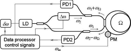
Figure 6.8 Schematic diagram of a typical RFOG.
It is seen that the resonance frequency shift does not depend on the fiber length of the ring, but a longer fiber is preferable since the resonance peak will be sharper and beneficial to higher detection resolution. Its sharpness also depends on the split ratio of the ring coupler, and reaches the maximum at the critical coupling (see Section 3.3).
A dead region at low angular velocity exists in simple RLG structures due to optical frequency lock-in induced by competition of longitudinal modes. Some methods were proposed to solve the problem. It is indicated theoretically and experimentally that the lock-in effect exists also in Brillouin RLGs. In addition, most parasitic effects existing in IFOG remain in BFOG, careful investigation and technical measures are needed [37].
Resonance fiber optic gyro (RFOG) makes use of the same effect in the fiber ring, but in passive operation mode. A typical close-loop scheme is shown in Figure 6.8, where the frequency of narrow linewidth LD beam is tuned ![]() by its pumping current, the LD beam is divided into two and injected into the fiber ring from its two ports. One of them is frequency shifted
by its pumping current, the LD beam is divided into two and injected into the fiber ring from its two ports. One of them is frequency shifted ![]() by an acousto-optic modulator (AOM). A PM is inserted in the ring to set the working bias to the quadrature point. Two photo detectors are used to receive the outputs of the fiber ring from its two ports. One of the detected signals is used to feedback control the laser frequency coincident with the ring resonance. The other is taken as the deviation induced by the rotation, to feedback control AOM to nullify the deviation signal, and then acquire the rotation velocity by the voltage on AOM. Thus the close-loop operation is fulfilled.
by an acousto-optic modulator (AOM). A PM is inserted in the ring to set the working bias to the quadrature point. Two photo detectors are used to receive the outputs of the fiber ring from its two ports. One of the detected signals is used to feedback control the laser frequency coincident with the ring resonance. The other is taken as the deviation induced by the rotation, to feedback control AOM to nullify the deviation signal, and then acquire the rotation velocity by the voltage on AOM. Thus the close-loop operation is fulfilled.
It is noted that the fiber ring is no longer an all-pass filter since a long fiber is usually used. Moreover, the Brillouin backscattering occurring in the fiber ring is a new and important loss factor. By neglecting the coupler loss, the transmission of the ring is expressed as
(6.13) ![]()
where ![]() is the finesse,
is the finesse, ![]() is the attenuation at resonances, and a loss factor
is the attenuation at resonances, and a loss factor ![]() is denoted. Based on the formulas, requirements of system designing, such as fiber length in the ring and beam split ratio of the coupler, are presented.
is denoted. Based on the formulas, requirements of system designing, such as fiber length in the ring and beam split ratio of the coupler, are presented.
The nonreciprocal factors and parasitic effects in IFOG affect also the performance of RFOG. The birefringence generates two sets of resonances; whereas the depolarized broadband source is not suitable to RFOG, and thus a polarization scrambled narrow line source is needed [24]. The influence of Rayleigh backscattering is more serious for the high coherence wave. Kerr effect becomes larger in the ring with higher finesse due to higher intensity inside the ring. More schemes and methods are being studied and developed.
6.2 FIBER OPTIC HYDROPHONE
The acoustic sensor is extremely important for all aspects of social life, from civil activities to military events. A famous example is the piezoelectric sonar. Since the first fiber hydrophone was reported in the 1970s [38–41], a variety of fiber optic hydrophones and geophones have been demonstrated, and related technologies are developing continuously. The fiber hydrophones are now available commercially and used widely in sea fishery, marine biology, seismic wave detection, oil well drilling, ultrasonic medicine, coast guarding, ship and submarine navigation, and so on. This section gives a brief introduction to fiber hydrophone technology, describes its basic structure and main technical problems.
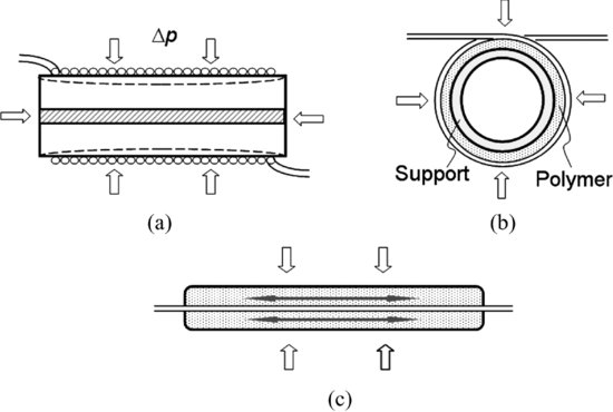
Figure 6.9 Transducers of acoustic pressure.
6.2.1 Basic Structures
The purpose of a hydrophone is to detect sound waves in water, and further to localize and distinguish the sound source. It is actually a dynamic pressure sensor; and multiple sensors form an array, or a system. The fiber hydrophones are categorized into active and passive sensors. The passive sensor includes generally two types: one is based on optical intensity variation [42,43], which has lower sensitivities; the other is the interferometric sensor based on the phase change. The active sensor makes use of the fiber laser. The hydrophone is basically composed of three main parts: (1) the sensor head, which transfers the pressure to fiber strains; (2) the interferometer, and the multiplex system; or the configuration of fiber laser; and (3) the signal interrogation and processing unit.
6.2.1.1 Sensor Head
Two typical structures of the sensor head are usually adopted [44–47]. Figure 6.9 shows a hollow mandrel with a fiber coil wound and fixed on it. The diameter of the mandrel will be deformed under the sound pressure, and an axial strain of the fiber occurs. To enhance its sensitivity, a polymer material with lower Young's Modulus may be placed underneath the fiber coil, as shown in Figure 6.9(b). Another structure is a fiber section coated with a thick and/or multiple layers, usually polymer materials with lower Young's Modulus and larger Poisson ratio, as shown in Figure 6.9(c). The polymer coating with a large cross section will expand axially under the pressure, and pull the fiber strained axially, if the bonding between the fiber and the coating is tight enough. The thick-coated fiber can also be used in the mandrel structure for enhanced sensitivity. The sensor unit may be further packaged into an acoustic resonant cavity to improve its frequency response [48].
It is no doubt necessary to design the mechanisms carefully; reference [45] and others give detailed analyses of the strains of some typical structures, based on the dynamic flexural plate theory. The phase change of a propagating light wave, induced by acoustic pressure, is expressed as
(6.14) ![]()
where the axial strain ez and the radial strain er are dependent on the structure of the pressure transduction mechanism and its materials, and proportional to the pressure. It is seen that a longer sensing fiber L is obviously advantageous to a higher sensitivity. The sensitivity of the hydrophone to the acoustic pressure p is generally defined as
(6.15) ![]()
in units of ![]() ; and the normalized sensitivity
; and the normalized sensitivity ![]() is used to characterize the sensitivity per optical path length.
is used to characterize the sensitivity per optical path length.
In active hydrophones, the most often used configuration is a fiber laser incorporated with a fiber Bragg grating, whose reflection peak wavelength is sensitive to the acoustic pressure, expressed as [49–52]
(6.16) ![]()
The gratings are usually imprinted in the active medium, such as erbium-doped fiber, to form a distributed feedback laser or a distributed Bragg reflection laser. A proper coating, as shown in Figure 6.9(c) will enhance the sensitivity of FBG to the acoustic pressure.
6.2.1.2 Interferometer and Interrogation
Hydrophones incorporated with different interferometers have been studied experimentally, including MZI, MI, SI, and FPI; the fiber gratings are also used for acoustic sensing [53]. Figure 6.10 shows schematically the interferometers. The sensor and the reference fiber coil are connected into the two beams of the interferometer, respectively. The reference fiber coil is used to set a proper biased optical path difference (![]() ). The output of the interferometer is written as
). The output of the interferometer is written as
Figure 6.10 Interferometers for acoustic sensing: (a) MZI; (b) MI; (c) SI; and (d) FPI and FBG.
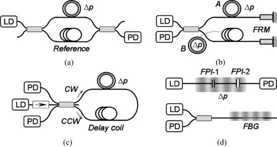
It is seen that a larger OPD gives a higher sensitivity, but a smaller linear dynamic range.
The SI is also sensitive to the sound wave [54] based on the temporal nonreciprocity, as analyzed in Section 5.5.1. To make use of the effect, a delay coil is inserted in the loop, making different time delays of the acoustic signal between CW and CCW propagations. A 3 × 3 coupler is used in the scheme to avoid quadrature point drift [55]. The Sagnac hydrophone has unique features: it is immune to the external disturbances of the acoustic frequency band detected; as a common-mode interferometer, a broadband source can be used, and some negative effects induced by narrow linewidth sources are removed; it eliminates drifts of working point, which occurs often in other interferometers.
A key technical issue is the interrogation of the required acoustic signals from large-scale sensor arrays and the retrieval of information from the noisy background and random drift. Some existing negative factors relate to the working principles of interferometer, such as polarization fading, temperature fluctuation, drift of working point, and phase noise. It is seen from (6.17) that the sensitivity depends on the phase bias; the highest sensitivity is obtained at ![]() . Several techniques are used to ensure the quadrature point; one of them is to add a PZT PM [56], with its driving voltage feedback adjusted to make the phase actively tracked. The scheme is called active homodyne, widely used in interferometric sensors. However, it is not convenient to put PZT components under water.
. Several techniques are used to ensure the quadrature point; one of them is to add a PZT PM [56], with its driving voltage feedback adjusted to make the phase actively tracked. The scheme is called active homodyne, widely used in interferometric sensors. However, it is not convenient to put PZT components under water.
Another scheme is the phase-generated carrier method (PGC) [57–59], by which a phase modulation is added in the interferometer with the modulation frequency higher than the acoustic frequency of interest, and with the modulation amplitude large enough to generate a larger side band. The phase modulated signal detected form the interferometer is expressed as
where V is the visibility of interference fringes, determined by the difference between the optical intensities of two beams; ![]() is the phase modulation amplitude, ω is the modulation frequency;
is the phase modulation amplitude, ω is the modulation frequency; ![]() is the detected signal, written as
is the detected signal, written as ![]() , with the acoustic frequency
, with the acoustic frequency ![]() and the external disturbance
and the external disturbance ![]() . The signal can be expanded as
. The signal can be expanded as

By mixing with the local oscillation of ω and ![]() , the low order harmonic components are obtained:
, the low order harmonic components are obtained:
(6.20a) ![]()
(6.20b) ![]()
(6.20c) ![]()
where ![]() ,
, ![]() , and
, and ![]() stand for mixing and filtering efficiencies for the three harmonics, which may not be necessarily the same, but can be calibrated. Formulas hold under the condition that the modulation frequency ω is higher than the band of detected acoustic signal.
stand for mixing and filtering efficiencies for the three harmonics, which may not be necessarily the same, but can be calibrated. Formulas hold under the condition that the modulation frequency ω is higher than the band of detected acoustic signal.
The acoustic signal to be detected can be calculated based on (6.19); however, the externally induced drift may result in signal fading and large errors. To remove the fading, time derivatives and cross-multiplying are made, resulting in
The detected signal can then be acquired by integrating (6.21) in data processing, which extends the linear dynamic range greatly. If the externally induced drift is much slower than the acoustic wave, the derivative of the phase can be approximated as
(6.22) ![]()
The acoustic wave does not necessarily have a single frequency; therefore, the frequency spectrum analyzer is needed in data processing. With a certain frequency ![]() , term
, term ![]() is expanded as
is expanded as
(6.23) 
and a similar expression for ![]() . It is seen that the variation of
. It is seen that the variation of ![]() will change the detected acoustic frequency spectrum. Other errors and noise sources, such as fluctuations of source power and visibility, should also be paid attention to in practice.
will change the detected acoustic frequency spectrum. Other errors and noise sources, such as fluctuations of source power and visibility, should also be paid attention to in practice.
Two methods are usually used to realize the phase modulation. One is by a piezo-electric modulator, which is not suitable for underwater applications. The other is with a modulated laser, externally by an optical waveguide phase modulator, for example, or internally by its driving current, if a laser diode is used. The latter is convenient in practical applications, and used widely. It is known that the lasing frequency of the laser diode can be modulated by the current, expressed as
(6.24) ![]()
The signal of interferometer depends on its OPD ![]() :
:
(6.25) ![]()
where ![]() is the length difference between sensing fiber and reference fiber. Correspondingly the parameters in (6.18) are written as
is the length difference between sensing fiber and reference fiber. Correspondingly the parameters in (6.18) are written as ![]() and
and ![]() . It is indicated that phase modulation can be realized by modulation of source frequency. The amplitude of equivalent phase modulation
. It is indicated that phase modulation can be realized by modulation of source frequency. The amplitude of equivalent phase modulation ![]() depends on the OPD and the modulation depth of laser frequency; therefore an unbalanced interferometer with a proper OPD is needed. The laser diode can be modulated easily and with high-speed response, making the system design freely. In addition, sensors with different OPD can be discriminated by scanning the laser frequency. It should be noted, however, that the output of the laser diode is modulated by the current simultaneously; this accompanied intensity modulation should be compensated. The PGC method has advantages of larger dynamic range, higher linearity, lower additive phase noise, and simpler electronics.
depends on the OPD and the modulation depth of laser frequency; therefore an unbalanced interferometer with a proper OPD is needed. The laser diode can be modulated easily and with high-speed response, making the system design freely. In addition, sensors with different OPD can be discriminated by scanning the laser frequency. It should be noted, however, that the output of the laser diode is modulated by the current simultaneously; this accompanied intensity modulation should be compensated. The PGC method has advantages of larger dynamic range, higher linearity, lower additive phase noise, and simpler electronics.
The interferometers are used also in the source unit and detection unit of the hydrophone system. Reference [60] describes a hydrophone with double Mach–Zehnder interferometers: one is used in the sensor head (at the “wet” end), and the other is used in the source unit (at the “dry” end). By actively modulating the latter to match the former, the signal fading is reduced. In the scheme, an acousto-optic modulator is used to generate two separate wavelengths. Such a configuration shows advantages: a laser source with a relatively short coherence length can be used; the OPD fluctuation of the sensor MZI can be compensated by using two probe wavelengths.
Polarization fluctuation is one of the major error sources. PMF is effective if the cost is not considered. The Faraday rotation mirror (FRM) is widely used to obviate the problem, as depicted in Figure 6.10(b); and depolarized or polarization scrambled optical beams are also helpful.
The hydrophone is often sensitive to the acceleration since it acts as an inertial force causing the fiber coil mandrel to deform, which should be distinguished from the acoustic signal. An effective method is to use paired sensors [45], as shown in Figure 6.10(b), where fiber coil B will be inserted as the reference. Two coils have the same sensitivity to the acceleration, but opposite sensitivities to the acoustic pressure. For example, the pressure is applied inside coil B as shown in the figure.
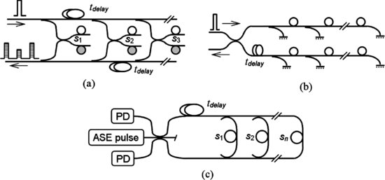
Figure 6.11 Typical hydrophone sensor arrays.
6.2.2 Sensor Arrays and Multiplexing
The practically used hydrophone and geophone must form a sensor array to detect the acoustic signal over a large area, for example, in several kilometers or more, whereas the spacing between the sensors may be only a few meters. On the other hand, sensor arrays packaged in a board are needed to detect the phase front of acoustic wave, in order to localize the sound source and to distinguish the target. It is an important subject to design and to build a large-scale sensor array and a multiplexing system [54,61–64], which should consider the requirements:
The typical configurations of a hydrophone array system are based on the parallel connection and series connection, and their combinations. Figure 6.11 shows several typical configurations: an MI array in parallel connection (a), an MI with multiple sensors in series connection (b), and a parallel connected SIs (c). MZI may be used instead of MI in configuration (a). Sensor arrays up to several tens of units are built by the configurations as one array module.
Large scale hydrophone networks must employ certain multiplexing technologies, basically the time division multiplex (TDM) and wavelength division multiplex (WDM) [62]. In TDM, some fiber delay lines are inserted in the path to distinguish and locate the sensor positions; in WDM, it is needed to use multiple optical add-drop multiplexers (OADM), as shown in Figures 6.12(a) and (b). For such large fiber systems, the loss of fiber and all optical components must be compensated by optical amplifiers (EDFA), shown in the figures. The characteristics and performances of sensor arrays and multiplexing systems are analyzed theoretically and simulated in reference [65]. This book will not go into detail here.
Figure 6.12 Large scale arrays with (a) TDM and (b) WDM technologies.

6.2.3 Low Noise Laser Source
The applications require a hydrophone with high performance, such as high phase resolution (![]() ), large linear dynamic range (107), small volume of sensor head, large-scale array covering large area, and low power consumption. The performance is finally limited by the noise, such as the shot noise and the thermal noise in detection and A/D converter, the thermal noise of interferometer fiber, the noise of optical amplifiers, and the noise of laser sources. The average power detected from the interferometer is typically around
), large linear dynamic range (107), small volume of sensor head, large-scale array covering large area, and low power consumption. The performance is finally limited by the noise, such as the shot noise and the thermal noise in detection and A/D converter, the thermal noise of interferometer fiber, the noise of optical amplifiers, and the noise of laser sources. The average power detected from the interferometer is typically around ![]() ; therefore, the laser noise is believed to give the greater contribution than others. The noise of laser source includes the relative intensity noise (RIN) and the phase noise. As an interferometric sensor, the effect of source phase noise on the detected signal is
; therefore, the laser noise is believed to give the greater contribution than others. The noise of laser source includes the relative intensity noise (RIN) and the phase noise. As an interferometric sensor, the effect of source phase noise on the detected signal is
where ![]() is the frequency deviation induced by the phase noise. It is seen that the lowest detectable phase change is proportional to linewidth of light source. It is estimated from (6.26) that for resolution of
is the frequency deviation induced by the phase noise. It is seen that the lowest detectable phase change is proportional to linewidth of light source. It is estimated from (6.26) that for resolution of ![]() , the phase noise (the frequency fluctuation) of
, the phase noise (the frequency fluctuation) of ![]() is required for the interferometer with OPD of ∼1 m. The intensity noise induced phase noise is given by
is required for the interferometer with OPD of ∼1 m. The intensity noise induced phase noise is given by ![]() , where
, where ![]() is the relative intensity noise of source power p, V is the visibility. Therefore the RIN should be reduced down to −130 dB/Hz for resolution of
is the relative intensity noise of source power p, V is the visibility. Therefore the RIN should be reduced down to −130 dB/Hz for resolution of ![]() .
.
Noise reduction is a hot topic in research and development; and high-quality lasers are now available commercially. Among the various laser schemes, the external cavity frequency-stabilized diode laser (ECDL), the erbium-doped fiber laser incorporated with the phase-shift Bragg grating (DFB-FL), and the diode-pumped Nd:YAG nonplanar ring laser (NPRL) may be the most attractive schemes. Reference [66] describes an DFB-FL with the master oscillator-power amplifier (MOPA) configuration; the RIN is suppressed down to −120 dB/Hz, by stabilizing the 980 nm pump power actively, and the phase noise is suppressed to ![]() at 1 kHz, by using an MZI as a frequency discriminator and a PZT element to tune the laser fiber. The linewidth of the single-frequency laser was reduced to 1 kHz.
at 1 kHz, by using an MZI as a frequency discriminator and a PZT element to tune the laser fiber. The linewidth of the single-frequency laser was reduced to 1 kHz.
The high-quality source must be carefully packaged to isolate any external vibration and temperature fluctuation. The performance of single-frequency lasers have continuously improved in recent years. Reference [67] gives a detailed review; demonstrating the capability of DFB fiber laser to resolve effective length change of ![]() at 2 kHz.
at 2 kHz.
The hydrophone technology has progressed greatly during the last three decades. The responsivity of a hydrophone sensor was reported to −127.5 dB relative to ![]() , better than those obtained from commercial piezoelectric hydrophones; the resolution reaches below ocean acoustic noise limitation; and large scale systems have been paved on the sea bed [63].
, better than those obtained from commercial piezoelectric hydrophones; the resolution reaches below ocean acoustic noise limitation; and large scale systems have been paved on the sea bed [63].
6.3 FIBER FARADAY SENSOR
As introduced in Section 3.4.4, the Faraday effect is widely used in a variety of applications, from optical components to astrophysics research. This section gives just a brief introduction to the sensors based on Faraday rotation.
6.3.1 Faraday Effect in Fiber
Faraday effect is attributed to the motion of electrons in the external electro-magnetic field. According to the elementary theory [68], it obeys the equation of motion under the Lorentzian force:
where m is the mass of electron, e is its charge and γ is the damping rate; ![]() stands for the quasi-elastic restoring force, relating with the electron's transitions. For a single frequency optical wave propagating in z-direction,
stands for the quasi-elastic restoring force, relating with the electron's transitions. For a single frequency optical wave propagating in z-direction, ![]() , its solution is expressed as
, its solution is expressed as
where ![]() is defined as the cyclotron frequency. It indicates that the electrons are moving in a helical manner in the magnetic filed. In case the damping is negligibly small, (6.28a) can be written as
is defined as the cyclotron frequency. It indicates that the electrons are moving in a helical manner in the magnetic filed. In case the damping is negligibly small, (6.28a) can be written as
where ![]() is the circularly polarized optical waves; the approximation in (6.28b) holds for the case when the optical frequency band is much higher than the electron's eigen resonance frequency. It is shown that the dielectric constant should now be expressed as a tensor; and the refractive indexes for the two circularly polarized waves are deduced to
is the circularly polarized optical waves; the approximation in (6.28b) holds for the case when the optical frequency band is much higher than the electron's eigen resonance frequency. It is shown that the dielectric constant should now be expressed as a tensor; and the refractive indexes for the two circularly polarized waves are deduced to
(6.29a) ![]()
where N is the electron number per unit volume. Their difference is
(6.29b) ![]()
The polarization rotation is obtained from the index difference
(6.30) ![]()
and the Verdet constant is expressed as
(6.31a) ![]()
Referring to the averaged index ![]() , it is transformed to
, it is transformed to
(6.31b) ![]()
indicating its relation with the dispersion. In case the magnetic field and/or the material are nonuniform along the optical path, the rotation is written as
(6.32) ![]()
The equations and formulas (6.27–6.32) give just a brief and simple explanation of the Faraday effect. The detailed understanding involves material structures and electron energy band properties; the Verdet constant should be multiplexed by the magneto-optical anomaly factor of the material. More physical phenomena and mechanisms related to Faraday effect have been investigated.
Fiber sensors and devices based on Faraday effect are generally divided into two types: (1) intrinsic and (2) extrinsic sensors. The former utilizes the Faraday effect of fiber itself, whereas the latter is composed of other materials with higher Verdet constant, coupled with fiber pigtails. The Faraday rotations were measured earlier in single mode fibers [69], and in PMFs [70]. The characteristics of Faraday effect were investigated and compared for different materials and for different wavelengths, giving the relation of Faraday rotation with the energy gap [71]. The Verdet constant of fused silica is measured as ![]() (T stands for Tesla) at 633 nm band. It is noted that the figure of merit, defined as
(T stands for Tesla) at 633 nm band. It is noted that the figure of merit, defined as ![]() , where α is the loss coefficient, is high for low loss silica fibers.
, where α is the loss coefficient, is high for low loss silica fibers.
Since the Faraday effect does not affect the strain state in fiber, the Faraday rotation can be simply combined with birefringence and torsion-induced rotation. In case of negligible torsion, the polarization evolution in a PMF with phase retardation of δ can be described [69,72]
(6.33) ![]()
where ![]() and
and ![]() are denoted with
are denoted with ![]() and
and ![]() . It is seen that an elliptically polarized wave results even if the input is a linearly polarized wave; and the polarization rotation, measured by rotation of the ellipsoid axis, is no longer the Faraday rotation
. It is seen that an elliptically polarized wave results even if the input is a linearly polarized wave; and the polarization rotation, measured by rotation of the ellipsoid axis, is no longer the Faraday rotation ![]() , and is even not proportional to it.
, and is even not proportional to it.
6.3.2 Electric Current Sensor Based on Faraday Rotation
It is attractive to use Faraday effect for the electric current sensor, since current monitoring and metering is of critical importance in the power industry, whereas the traditional transformer becomes cumbersome and costs increasingly more to meet the strict requirement of insulation for high voltages. That is why the optical fiber current sensor is so attractive. The principle of the Faraday current sensor is understandable: the Faraday rotation of the wave in the fiber loop round a power cable is proportional to the line integral of the magnetic field; it is just equal to the current in the wire, according to Ampere theorem. In practical applications, however, several technical problems have to be dealt with and solved.
6.3.2.1 Basic Configurations
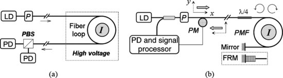
Faraday current sensors have been developed for practical field applications. Figure 6.13(a) gives a conceptual diagram to illustrate its operation [73], where the fiber loop may be composed of several circles to increase the rotation angle. The source light is polarized by the polarizer (P); the returned wave is analyzed by a polarization beam splitter (PBS), and received by two detectors. The Faraday rotation is acquired from the two signals P1 and P2:
Figure 6.13 Faraday sensor: (a) basic structure and (b) reflective sensor.
(6.34) ![]()
where C is a constant, dependent on perfectness of the polarizer and PBS. The Faraday rotation is written as ![]() , where N is the circle number,
, where N is the circle number, ![]() is the current to be measured.
is the current to be measured.
Figure 6.14 (a) Faraday sensor based on Sagnag loop and (b) passive fiber phase retard.

This plain structure has problems of instability and external disturbances. The sensor is then improved greatly for practical applications. Figure 6.13(b) shows schematically a structure well developed [74–76], in which PMF loop is used and a mirror is set at the end of the fiber loop, and the doubled Faraday rotation is measured in the reflected beam, ![]() . The configuration brings about another merit, that is, reciprocal interferences, such as additional birefringence, can be cancelled. The end mirror can be replaced by a FRM to remove the external disturbances more effectively. A
. The configuration brings about another merit, that is, reciprocal interferences, such as additional birefringence, can be cancelled. The end mirror can be replaced by a FRM to remove the external disturbances more effectively. A ![]() wave plate is inserted to convert the input wave to a circularly polarized wave, which in combination with the polarizer plays the role of isolator; and the polarizer plays also a role of polarization analyzer for the reflected beam. A phase modulator (PM) is inserted to set the quadrature working point and to suppress the noise, similar to the method in fiber optic gyros.
wave plate is inserted to convert the input wave to a circularly polarized wave, which in combination with the polarizer plays the role of isolator; and the polarizer plays also a role of polarization analyzer for the reflected beam. A phase modulator (PM) is inserted to set the quadrature working point and to suppress the noise, similar to the method in fiber optic gyros.
Another configuration is based on SI, as shown in Figure 6.14 [74], in which more reciprocal interferences can be removed. The detected Faraday rotation θ is doubled once again by CW and CCW interference: ![]() . The depolarized Sagnac loop is also used for current sensing [77]. It is noted that the
. The depolarized Sagnac loop is also used for current sensing [77]. It is noted that the ![]() wave plate used in the structures of Figures 6.13(b) and 6.14(a) is a passive device, since it is located at the high voltage position, together with the sensing fiber coil, and is impossible to adjust electrically or manually. The fixed quarter wavelength waveplate can be fabricated by orthogonally splicing a PMF section [75], as schematically shown in Figure 6.14(b).
wave plate used in the structures of Figures 6.13(b) and 6.14(a) is a passive device, since it is located at the high voltage position, together with the sensing fiber coil, and is impossible to adjust electrically or manually. The fixed quarter wavelength waveplate can be fabricated by orthogonally splicing a PMF section [75], as schematically shown in Figure 6.14(b).
Reference [76] summarizes the technologies of the Faraday sensor as one of the polarimetric optical fiber sensors. It is possible to construct a fiber sensor system composed of multiple Faraday sensors to meet practical demand. References [77–79] propose some configurations and discuss their interrogation and other technical problems. The polarization OTDR can also be used to detect distributed current signals [80].
6.3.2.2 Precision and Stability
As a current meter and monitor, the Faraday sensor must be highly precise, stable, and have a dynamic range large enough. For example, the nominal primary current is 1,000 A, the dynamic range of 50∼1,200 A is required with the measurement precision of 0.5% [73].
Temperature dependence is the main factor of instability. It was measured that the Verdet constant varies with temperature, ![]() for silica at 633 nm; and the thermal expansion of fiber should be taken into account, fortunately its contribution is negligibly small for silica [81]. Materials other than silica were investigated, such as flint glass and BK7 glass [72,81,82]. It is found that the thermal stability of diamagnetic materials is much better than that of paramagnetic materials, though the latter has a higher Verdet constant [73]. The temperature dependence of optical components, such as the coupler and the phase retarder, needs to be dealt with carefully. Mechanical stability is another factor, including influence of vibration and thermal strains; the fiber loop should be packaged robustly [74,75,83].
for silica at 633 nm; and the thermal expansion of fiber should be taken into account, fortunately its contribution is negligibly small for silica [81]. Materials other than silica were investigated, such as flint glass and BK7 glass [72,81,82]. It is found that the thermal stability of diamagnetic materials is much better than that of paramagnetic materials, though the latter has a higher Verdet constant [73]. The temperature dependence of optical components, such as the coupler and the phase retarder, needs to be dealt with carefully. Mechanical stability is another factor, including influence of vibration and thermal strains; the fiber loop should be packaged robustly [74,75,83].
The Verdet constant is a function of optical frequency (6.31a and 6.31b), and is dependent on material property. It was measured [84,85] that roughly the Verdet constant is proportional to the square of frequency: ![]() (λ in
(λ in ![]() m). Therefore, shorter wavelength sources are preferable; in practice, the diode laser at 800 nm band is often used.
m). Therefore, shorter wavelength sources are preferable; in practice, the diode laser at 800 nm band is often used.
The instability comes also from the lead fiber, which usually cannot be fixed in position tightly and often suffers vibration and sway, causing the polarization to be disturbed. PMF has proved helpful in reducing the influence [75,83]. A depolarized sensor structure is proposed and studied experimentally [78]. A circular-polarization-maintaining optical fiber is shown to have better immunity against the disturbance of twisting [86].
The external disturbances give serious influence, especially for direct current sensing. In case the sensor is used for alternating currents, the Faraday rotation is modulated by the AC frequency: ![]() ; and the detected signal is written as
; and the detected signal is written as
(6.35) ![]()
The Faraday rotation can then be calculated by a frequency SA, whereas the external disturbances out of the AC frequency are removed greatly. The signal processing also gives out data on the AC frequency and its phase, which are important parameters in the power industry. On the other hand, linear signals in a large dynamic range are obtained by data processing. Schemes of a close loop system with an adjustable PM are developed for the linear signal [75,78].
Faraday effect is also widely used for fiber optic devices, especially the optical isolator [70,72]. Detailed characteristics and analyses can be found in the literature.
6.4 FIBER SENSORS BASED ON SURFACE PLASMON EFFECT
The detection of chemical and biochemical samples is important in various aspects of human life and industrial production. Quite a lot of methods have been developed. Among them optical fiber sensors have attractive features. This section gives a brief introduction to the sensors based on surface plasmon effect.
6.4.1 Surface Plasmon Effect
Electrons in metals and semiconductors can move freely, their behaviors in an electromagnetic field show properties of the plasma. The optical constants of metal are analyzed in [68]. By referring to Equation (6.27), the motion of electrons in cases where there is no external magnetic field, is described as
(6.36) ![]()
The dielectric constant is expressed as
(6.37) ![]()
where Pion and ![]() stands for the contributions to electric polarization and dielectric constant from ions and the lattice, respectively. The real and imaginary parts of the dielectric constant are then written as
stands for the contributions to electric polarization and dielectric constant from ions and the lattice, respectively. The real and imaginary parts of the dielectric constant are then written as
(6.38a) ![]()
(6.38b) ![]()
The expressions are just the well-known Drude formula, considering the damping rate γ is related with the conductivity σ by relation of ![]() . It is shown that
. It is shown that ![]() is negative for low frequency and positive for high frequency, and reaches zero at frequency of
is negative for low frequency and positive for high frequency, and reaches zero at frequency of ![]() , which is termed the state of plasma resonance. It is seen that the larger the electron concentration, the higher is the plasma resonance frequency. The resonance frequency of a metal with high conductivity is in the ultraviolet band, much higher than that of semiconductors. At the resonance the imaginary part plays the main role in determining its optical behavior; and the imaginary part of the index reaches its maximum, meaning a loss peak. The refractive index of metals is a complex, usually with
, which is termed the state of plasma resonance. It is seen that the larger the electron concentration, the higher is the plasma resonance frequency. The resonance frequency of a metal with high conductivity is in the ultraviolet band, much higher than that of semiconductors. At the resonance the imaginary part plays the main role in determining its optical behavior; and the imaginary part of the index reaches its maximum, meaning a loss peak. The refractive index of metals is a complex, usually with ![]() and
and ![]() in the visible and infrared band. The measured data of the metals are given in reference [68]. Reference [87] gives a formula for the dielectric constant with dependence on wavelength:
in the visible and infrared band. The measured data of the metals are given in reference [68]. Reference [87] gives a formula for the dielectric constant with dependence on wavelength:
(6.39) ![]()
The parameters are measured as ![]()
![]() m and
m and ![]()
![]() m for gold;
m for gold; ![]()
![]() m and
m and ![]()
![]() m for silver. Thus the di- electric constants at 1,550 nm band are calculated as
m for silver. Thus the di- electric constants at 1,550 nm band are calculated as ![]() . and
. and ![]() . The dielectric constants measured for other wavelengths are reported:
. The dielectric constants measured for other wavelengths are reported: ![]() at 633 nm [88],
at 633 nm [88], ![]() at 830 nm [89].
at 830 nm [89].
It is known that in the total internal reflection at the interface between two media the optical wave penetrates the interface, being an evanescent field with amplitude of ![]() , where x is perpendicular to the interface. The depth is deduced as
, where x is perpendicular to the interface. The depth is deduced as
(6.40) 
where ![]() is the incident angle from medium n1. When a thin layer of metal is coated on the surface of a medium, or a metal is placed in the evanescent field area, the electrons will be driven by the field, causing an electron density oscillation and a secondary electromagnetic wave, called a surface plasmon wave (SPW). Obviously the plasmon intensity depends on the frequency, and reaches resonance at
is the incident angle from medium n1. When a thin layer of metal is coated on the surface of a medium, or a metal is placed in the evanescent field area, the electrons will be driven by the field, causing an electron density oscillation and a secondary electromagnetic wave, called a surface plasmon wave (SPW). Obviously the plasmon intensity depends on the frequency, and reaches resonance at ![]() . This is the basic physical picture of surface plasmon resonance (SPR).
. This is the basic physical picture of surface plasmon resonance (SPR).
The TE and TM incident waves have different characteristics at the interface between the metal and the dielectric medium. The electric field of the TE wave is in y-direction, perpendicular to the incident plane; it suffers larger loss in the metal layer. In other words, the TE wave is screened from entering the metal, so that E(TE)y at the interface is minimized with a zero evanescent field. The conclusion can also be derived from the boundary conditions of the electric and magnetic fields. The TM wave has components in x- and z-directions; the x-component will penetrate into the thin metal layer. This behavior is similar to the reflections of P- and S-components of the incident beam at medium surface.
The property of SPW is investigated [87–90] by analyzing the electromagnetic wave at the interface, as shown in Figure 6.15(a), where region of x<0 is the metal; the dielectric constant ![]() is a real with a negligible loss in region x>0. The electric fields of a TM wave are written as
is a real with a negligible loss in region x>0. The electric fields of a TM wave are written as
Figure 6.15 Illustration of SPW.

(6.41a) ![]()
(6.41b) ![]()
It is deduced from ![]() that
that ![]() and
and ![]() . The boundary conditions require E1z=E2z and
. The boundary conditions require E1z=E2z and ![]() ; therefore,
; therefore, ![]() . By substituting
. By substituting ![]() and
and ![]() , it is deduced that
, it is deduced that

Its real and imaginary parts are deduced to be
(6.43a) 
(6.43b) 
where ![]() . The x-components of wave vectors are obtained:
. The x-components of wave vectors are obtained:
(6.44a) ![]()
(6.44b) ![]()
Both of them are complex; for the wave confound at two sides of the interface, the imaginary part of k1x must be positive, whereas that of k2x must be negative. This condition is ensured by the large negative ![]() of the metal. The real and imaginary parts of k1x are deduced to be
of the metal. The real and imaginary parts of k1x are deduced to be
(6.45a) 
(6.45b) 
The formulas can be approximated under condition of ![]()
![]() and the propagation constant in z-direction is obtained as
and the propagation constant in z-direction is obtained as
(6.46a) ![]()
(6.46b) ![]()
It is seen that SPW decays in z-direction, and the attenuation depends on the optical frequency.
For a thin metal layer, SPW will occur on both of its sides, as shown in Figure 6.15(b). The detailed analysis involves a three-layer waveguide with a high loss core [90]. Or phenomenally, ![]() in (6.42) is regarded as a composite dielectric constant of the metal and medium
in (6.42) is regarded as a composite dielectric constant of the metal and medium ![]() . In practical applications, medium
. In practical applications, medium ![]() is usually a fluid; the chemical and biochemical molecules being detected are solved in the fluid and adsorbed partly on the metal surface, contributing to the composite dielectric constant.
is usually a fluid; the chemical and biochemical molecules being detected are solved in the fluid and adsorbed partly on the metal surface, contributing to the composite dielectric constant.
6.4.2 Sensors Based on SPW
The SPW is generally excited by the evanescent field in total internal reflection (TIR). Two basic configurations have been developed, as shown in Figure 6.16. Figure 6.16(a) is the Kretschmann configuration, with the evanescent field tunneling through a thin metal layer; and Figure 6.16(b) is the Otto configuration, with the evanescent field extending across a dielectric gap to excite the plasmon on the metal surface [90].
Figure 6.16 Excitations of SPW: (a) Kretschmann and (b) Otto configurations.

The total internal reflection occurring at one of the surfaces of the glass prism is usually utilized for the SPW sensor. The prism surface is coated with a metal layer, or is pressed by a metal plate. An adsorbing layer may be coated on the metal layer in configuration (a), to enhance the sensitivity and the selectivity of the sensor. The reflected beam suffers certain attenuation caused by the loss of specimen being tested. Characteristics of the configurations can be analyzed as the substrate mode of a three layer waveguide, with a parameter of incident beam wavevector ![]() ; or by the theoretical model of multi-layer dielectric coating and attenuated total reflection (ATR), as done in [91,92].
; or by the theoretical model of multi-layer dielectric coating and attenuated total reflection (ATR), as done in [91,92].
The characteristics of ATR are usually interrogated by two methods: measurement of the attenuation varied with the wavelength, and varied with the incident angle. Figures 6.17(a) and (b) show the two methods schematically, where Kretschmann and Otto configurations are exchangeable, that is, both of them can be characterized by the spectrum analysis, or by angle scanning. Reference [91] gives detailed analysis and curve fitting equations. Such apparatus, containing necessary optical components, such as polarizers, and electronics, are already commercialized [93–95].
Figure 6.17 Measurements of ATR: (a) varied with wavelength and (b) varied with incident angle.

The development of optical waveguide devices and fiber devices, waveguide and fiber SPW sensors has become a hot topic of R&D, because the evanescent field exists already in waveguide structures, and the fiber sensor is attractive for its small size, low cost, and ease of usage. References [88,96] describe planar waveguide SPW sensors on glass slides. Quite a number of papers show research on optical fibers. Several schemes have been demonstrated. One of them is based on a thinned fiber [92,97–99], as depicted in Figure 6.18(a). The other has D-shaped fibers [89,100,101], as shown in Figure 6.18(b).
Figure 6.18 SPW sensors with (a) thinned fiber and (b) D-shaped fiber.

Fiber grating SPW sensors has attracted wide interest [101–105]. The long-period gratings have been used to detect the index of the environmental medium; the SPW sensor with metal-coated LPFG shows more functions and improved performance. Several structures are proposed to make SPW sensors with the FBG type, such as thinned and D-shaped structures. A hollow core fiber with metal coating in the inner wall is fabricated as a special SPW sensor [102]; and the tilted FBG is also studied for the SPW sensor applications since quite a lot of cladding modes are excited in the structure [105]. It is noticed that the fiber taper has geometry of thinned tip or a thinned waist, and the core mode is expanded into the cladding region; such features are thought favorable for SPW sensing, and the sensor with a small tip provides convenience in applications [106,107].
Two measurands are of concern in chemical and biochemical sensors: identity of the specimen and the quantity (concentration). It is difficult to fulfill such a task in a single measurement. Reference [93] proposes a self-referencing SPR sensor, which uses a TIR prism with two region coatings: gold layer and gold/Ta2O5 double layer, as shown in Figure 6.19(a) and separate SPR peaks are measured in the spectrum. Reference [108] proposes a special prism, shown in Figure 6.19(b), by which SPR spectrum with two different incident angles is obtained in a single measurement.
Figure 6.19 Schemes of SPW sensor: (a) double region and (b) two angles.

An issue of especial concern is how to enhance the sensitivity of the sensor. Selection of the metal is important for the SPW sensors. It is seen that the dielectric constant of silver has a larger negative real part than gold, which is favorable for excitation of the surface plasmon [97]. However, the chemical stability of gold is better than silver. Therefore a Au/Ag double layer is preferable [99]. A composite layer with multiple dielectric coating and organic cap layer, such as thiol material, is also proposed and demonstrated.
It is also found experimentally that a metal coating with rough surface is beneficial to the SPW excitation than that with smooth surface. Moreover, the surface plasmon will enhance fluorescence emission, which is utilized to develop a new sensor, named the surface plasmon enhanced fluorescence sensor (SPFS) [109].
Similar structures are used in surface enhanced Raman spectroscope (SERS) [110]. In the SERS sensors, nanometer gold balls are deposited onto the surface of the fiber or planar waveguide; and sharp and strong Raman signals are measured. SERS is an attractive topic, but beyond the scope of this book.
PROBLEMS
6.1 How does the phase shift of the Sagnac loop depend on the angular velocity of rotation? How dos it depend on the area of loop? Deduce the formula of the Sagnac phase shift.
6.2 What roles does a PM play in IFOG? How do you set the modulation frequency?
6.3 Why will Rayleigh scattering in the loop fiber induce parasitic signals? How do you reduce the effect?
6.4 Why and how does the Kerr effect induce parasitic signals?
6.5 Why do polarization properties induce noise? Why does the cross-coupling between the two polarization modes play an important role? How do you reduce the effect?
6.6 Why do temperature distribution and its temporal variation in the fiber spool induce nonreciprocity? How do you reduce the effect?
6.7 Why can the fiber optic gyro be used to localize the latitude?
6.8 Describe the structures of IFOG and RFOG. What are their differences and features?
6.9 Describe the most often used structures of acoustic pressure transduction.
6.10 Which interferometers are mostly used in hydrophones? Describe their structures.
6.11 Why should a modulator be inserted in the interferometer of a hydrophone? What is the PGC method? Deduce its basic formulas.
6.12 Why is the sensor array important in practical applications? How do you interrogate the signals from the sensor array?
6.13 Why must a low noise laser source be used in high-sensitivity hydrophones?
6.14 Why can the Faraday effect be used as a current sensor? Deduce the formula of polarization rotation varied with the current.
6.15 Describe the most often used configurations of fiber Faraday sensors. What factors affect the performance of the sensor? How do you improve the precision and stability of the sensor?
6.16 Describe the property of the metal dielectric constant. What is the difference between properties of metal and dielectric medium? What is the SPW? How do you excite the SPW?
6.17 Explain the total internal reflection and attenuated total reflection. Describe the basic structures of SPW sensors. How does the SPW sensor detect index change? How does it detect chemical and biochemical specimens?
REFERENCES
1. Bergh RA, Lefevre HC, Shaw HJ. All-single-mode fiber-optic gyroscope. Optics Letters 1981; 6: 198–200.
2. Lefvère HC. The Fiber-Optic Gyroscope. London, Boston: Artech House Inc., 1993.
3. Sanders GA, Szafraniec B, Liu RY, Laskoskie C, Strandjord L, Weed G. Fiber optic gyros for space, marine and aviation applications. Proceeding of SPIE 1996; 2837: 61–71.
4. Lee B. Review of the present status of optical fiber sensors. Optical Fiber Technology 2003; 9: 57–79.
5. Culshaw B. The optical fibre Sagnac interferometer: an overview of its principles and applications. Measurement Science and Technology 2006; 17: R1–R16.
6. Leeb WR, Schiffner G, Scheiterer E. Optical fiber gyroscopes: Sagnac or Fizeau effect? Applied Optics 1979; 18: 1293–1295.
7. Arditty HJ, Lefevre HC. Sagnac effect in fiber gyroscopes. Optics Letters 1981; 6: 401–403.
8. Bergh RA, Lefevre HC, Shaw HJ. An overview of fiber-optic gyroscopes. Journal of Lightwave Technology 1984; 2: 91–107.
9. Ruffin PB. Fiber optic gyroscope sensors. Section 8 of Fiber Optic Sensor, edited by Yin S, Ruffin PB, Francis TS, Yu FTS. Second Edition. Boca Raton, FL: CRC Press, Taylor & Francis Group, 2008.
10. Bergh RA, Lefevre HC, Shaw HJ. All-single-mode fiber-optic gyroscope with long-term stability. Optics Letters 1981; 6: 502–504.
11. Moeller RP, Burns WK, Frigo NJ. Open-loop output and scale factor stability in a fiber-optic gyroscope. Journal of Lightwave Technology 1989; 7: 262–269.
12. Trommer GF, Poisel H, Buhler W, Hartl E, Muller R. Passive fiber optic gyroscope. Applied Optics 1990; 29: 5360–5365.
13. Kim BY, Shaw HJ. Gated phase-modulation approach to fiber-optic gyroscope with linearized scale factor. Optics Letters 1984; 9: 375–377.
14. Pavlath GA. Closed-loop fiber optic gyros. Proceeding of SPIE 1996; 2837: 46–60.
15. Cutler CC, Newton SA, Shaw HJ. Limitation of rotation sensing by scattering. Optics Letters 1980; 5: 488–490.
16. Bohm K, Russer P, Weidel E, Ulrich R. Low-noise fiber-optic rotation sensing. Optics Letters 1981; 6: 64–66.
17. Bohm K, Marten P, Petermann K, Weidel E, Ulrich R. Low-drift fiber gyro using a superluminescent diode. Electronics Letters 1981; 17: 352–353.
18. Peng GD, Huang SY, Lin ZQ. Intensity noise characteristics of lasers in fiber-optic gyroscopes. Optics Letters 1987; 12: 434–436.
19. Wysocki PF, Digonnet MJF, Kim BY, Shaw HJ. Characteristics of erbium-doped superfluorescent fiber sources for interferometric sensor applications. Journal of Lightwave Technology 1994; 12: 550–567.
20. Bergh RA, Culshaw B, Cutler CC, Lefevre HC, Shaw HJ. Source statistics and the Kerr effect in fiber-optic gyroscopes. Optics Letters 1982; 7: 563–565.
21. Agrawal GP. Nonlinear Fiber Optics. Singapore: Elsevier Science, 2004.
22. Burns WK, Moeller RP, Villarruel CA, Abebe M. Fiber-optic gyroscope with polarization-holding fiber. Optics Letters 1983; 8: 540–542.
23. Carrara SLA, Kim BY, Shaw HJ. Bias drift reduction in polarization-maintaining fiber gyroscope. Optics Letters 1987; 12: 214–216.
24. Chien PY, Pan CL. Fiber-optic gyroscopes based on polarization scrambling. Optics Letters 1991; 16: 189–190.
25. Szafraniec B, Sanders GA. Theory of polarization evolution in interferometric fiber-optic depolarized gyros. Journal of Lightwave Technology 1999; 17: 579–590.
26. Shupe DM. Fiber resonator gyroscope: sensitivity and thermal nonreciprocity. Applied Optics 1981; 20: 286–289.
27. Ruffin PB, Lofts C, Sung CC, Page JL. Reduction of nonreciprocity noise in wound fiber optic interferometers. Optical Engineering 1994; 33: 2675–2679.
28. Lofts CM, Ruffin PB, Parker M, Sung CC. Investigation of the effects of temporal thermal-gradients in fiber optic gyroscope sensing coils. Optical Engineering 1995; 34: 2856–2863.
29. Sawyer J, Ruffin PB, Sung CC. Investigation of the effects of temporal thermal gradients in fiber optic gyroscope sensing coils, part 2. Optical Engineering 1997; 36: 29–34.
30. Ruffin PB, Baeder J, Sung CC. Study of ultraminiature sensing coils and the performance of a depolarized interferometric fiber optic gyroscope. Optical Engineering 2001; 40: 605–611.
31. Kim DH, Kang JU. Sagnac loop interferometer based on polarization maintaining photonic crystal fiber with reduced temperature sensitivity. Optics Express 2004; 12: 4490–4495.
32. Bohm K, Petermann K, Weidel E. Sensitivity of a fiber optic gyroscope to environmental magnetic fields. Optics Letters 1982; 7: 180–182.
33. Hotate K, Tabe K. Drift of an optical fiber gyroscope caused by the Faraday effect: influence of the earth's magnetic field. Applied Optics 1986; 25: 1086–1092.
34. Ojeda L, Chung H, Borenstein J. Precision-calibration of fiber-optic gyroscopes for mobile robot navigation. Proceedings of the IEEE International Conference on Robotics and Automation 2000: 2064–2069, San Francisco. vol 4.
35. Zheng J. Birefringent fibre frequency-modulated continuous-wave Sagnac gyroscope. Electronics Letters 2004; 40: 1520–1522.
36. Zarinetchi F, Smith SP, Ezekiel S. Stimulated Brillouin fiber-optic laser gyroscope. Optics Letters 1991; 16: 229–231.
37. Tanaka Y, Yamasaki S, Hotate K. Brillouin fiber-optic gyro with directional sensitivity. IEEE Photonics Technology Letters 1996; 8: 1367–1369.
38. Cole JH, Johnson RL, Bhuta PG. Fiber-optic detection of sound. Journal of Acoustical Society America 1977; 62: 1136–1138.
39. Bucaro JA, Dardy HD, Carome EF. Fiber-optic hydrophone. Journal of Acoustical Society America 1977; 62: 1302–1304.
40. Shajenko P, Flatley JP, Moffett MB. Fiberoptic hydrophone sensitivity. Journal of Acoustical Society America 1978; 64: 1286–1288.
41. Stanton TK, Pridham RG, Mccollough WV, Sanguinetti MP. Fiber-optic hydrophone noise-equivalent pressure. Journal of Acoustical Society America 1979; 66: 1893–1894.
42. Spillman WB, Gravel RL. Moving fiber-optic hydrophone. Optics Letters 1980; 5: 30–31.
43. Rashleigh SC. Acoustic sensing with a single coiled monomode fiber. Optics Letters 1980; 5: 392–394.
44. Giallorenzi TG, Bucaro JA, Dandridge A, Sigel GH, Cole JH, Rashleigh SC, Priest RG. Optical fiber sensor technology. IEEE Journal of Quantum Electronics 1982; 18: 626–665.
45. Garrett SL, Brown DA, Beaton BL, Wetterskog K, Serocki J. A general-purpose fiber-optic hydrophone made of castable epoxy. Proceeding of SPIE 1990; 1367: 13–29.
46. Dandridge A, Cogdell GB. Fiber optic sensors for navy applications. IEEE LCS 1991; 2: 81–89.
47. Nash P. Review of interferometric optical fibre hydrophone technology. IEE Proceedings-Radar Sonar and Navigation 1996; 143: 204–209.
48. Wang Z, Hu Y, Meng Z, Ni M. Fiber-optic hydrophone using a cylindrical Helmholtz resonator as a mechanical anti-aliasing filter. Optics Letters 2008; 33: 37–39.
49. Beverini N, Falciai R, Maccioni E, Morganti M, Sorrentino F, Trono C. Developing fiber lasers with Bragg reflectors as deep sea hydrophones. Annals of Geophysics 2006; 49: 1157–1165.
50. Bagnoli PE, Beverini N, Falciai R, Maccioni E, Morganti M, Sorrentino F, Stefani F, Trono C. Development of an erbium-doped fibre laser as a deep-sea hydrophone. Journal of Optics A-Pure and Applied Optics 2006; 8: S535–S539.
51. Hill DJ, Nash PJ, Jackson DA, Webb DJ, O'Neill SF, Bennion I, Zhang L. A fiber laser hydrophone array. Proceedings SPIE 1999; 3860: 55–66.
52. Hill DJ, Hodder B, De Freitas J, Thomas SD, Hickey L. DFB fibre-laser sensor developments. Proceedings SPIE 2005; 5855: 904–907.
53. Peng GD, Chu PL. Optical fiber hydrophone systems, Section 9 of Fiber Optic Sensor, edited by Yin S, Ruffin PB, Yu FTS. Second Edition. Boca Raton, FL: CRC Press, Taylor & Francis Group, 2008.
54. Digonnet MJF, Vakoc BJ, Hodgson CW, Kino GS. Acoustic fiber sensor arrays. Proceedings SPIE 2004; 5502: 39–50.
55. Koo KP, Tveten AB, Dandridge A. Passive stabilization scheme for fiber interferometers using (3 × 3) fiber directional couplers. Applied Physics Letters 1982; 41: 616–618.
56. Fritsch K, Adamovsky G. Simple circuit for feedback stabilization of a single-mode optical fiber interferometer. Review of Scientific Instruments 1981; 52: 996–1000.
57. Dandridge A, Tveten AB, Giallorenzi TG. Homodyne demodulation scheme for fiber optic sensors using phase generated carrier. IEEE Journal of Quantum Electronics 1982; 18: 1647–1653.
58. Kersey AD, Dandridge A, Tveten AB. Time-division multiplexing of interferometric fiber sensors using passive phase-generated carrier interrogation. Optics Letters 1987; 12: 775–777.
59. Dandridge A, Tveten AB, Kersey AD, Yurek AM. Multiplexing of interferometric sensors using phase carrier techniques. Journal of Lightwave Technology 1987; 5: 947–952.
60. Lim TK, Zhou Y, Lin Y, Yip YM, Lam YL. Fiber optic acoustic hydrophone with double Mach-Zehnder interferometers for optical path length compensation. Optics Communications 1999; 159: 301–308.
61. Nash P, Cranch G, Cheng LK, de Bruijn D, Crowe I. A 32 element TDM optical hydrophone array. Proceedings SPIE 1998; 3483: 238–242.
62. Cranch GA, Nash PJ. Large-scale multiplexing of interferometric fiber-optic sensors using TDM and DWDM. Journal of Lightwave Technology 2001; 19: 687–699.
63. Cranch GA, Nash PJ, Kirkendall CK. Large-scale remotely interrogated arrays of fiber-optic interferometric sensors for underwater acoustic applications. IEEE Sensors Journal 2003; 3: 19–30.
64. Cranch GA, Kirkendall CK, Daley K, Motley S, Bautista A, Salzano J, Nash PJ, Latchem J, Crickmore R. Large-scale remotely pumped and interrogated fiber-optic interferometric sensor array. IEEE Photonics Technology Letters 2003; 15: 1579–1581.
65. Brooks JL, Moslehi B, Kim BY, Shaw HJ. Time-domain addressing of remote fiber-optic interferometric sensor arrays. Journal of Lightwave Technology 1987; 5: 1014–1023.
66. Cranch GA. Frequency noise reduction in erbium-doped fiber distributed-feedback lasers by electronic feedback. Optics Letters 2002; 27: 1114–1116.
67. Cranch GA, Flockhart GMH, Kirkendall CK. Distributed feedback fiber laser strain sensors. IEEE Sensors Journal 2008; 8: 1161–1172.
68. Born M, Wolf E. Principles of Optics. Seventh Edition. Cambridge: Cambridge University Press, 1999.
69. Smith AM. Polarization and magneto-optic properties of single-mode optical fiber. Applied Optics 1978; 17: 52–56.
70. Stolen RH, Turner EH. Faraday rotation in highly birefringent optical fibers. Applied Optics 1980; 19: 842–845.
71. Munin E, Roversi JA, Villaverde AB. Faraday effect and energy gap in optical-materials. Journal of Physics D-Applied Physics 1992; 25: 1635–1639.
72. Shiraishi K, Sugaya S, Kawakami S. Fiber Faraday rotator. Applied Optics 1984; 23: 1103–1106.
73. Papp A, Harms H. Magneto-optical current transformer. 1: principles. Applied Optics 1980; 19: 3729–3734.
74. Bohnert K, Gabus P, Nehring J, Brandle H. Temperature and vibration insensitive fiber-optic current sensor. Journal of Lightwave Technology 2002; 20: 267–276.
75. Bohnert K, Gabus P, Kostovic J, Brandle H. Optical fiber sensors for the electric power industry. Optics and Lasers in Engineering 2005; 43: 511–526.
76. Michie C. Polarimetric optical fiber sensors. Section 3 of Fiber Optic Sensor, edited by Yin S, Ruffin PB, Francis TS, Yu FTS. Second Edition. CRC Press, Taylor & Francis Group, 2008.
77. Lin H, Huang SC. Fiber-optics multiplexed interferometric current sensors. Sensors and Actuators A 2005; 121: 333–338.
78. Takahashi M, Sasaki K, Ohno A, Hirata Y, Terai K. Sagnac interferometer-type fibre-optic current sensor using single-mode fibre down leads. Measurement Science and Technology 2004; 15: 1637–1641.
79. Guan ZG, He S. Coherence multiplexing system based on asymmetric mach-zehnder interferometers for Faraday sensors. IEEE Photonics Technology Letters 2007; 19: 1907–1909.
80. Kim BY, Park D, Choi SS. Use of polarization-optical time domain reflectometry for observation of the Faraday effect in single-mode fibers. IEEE Journal of Quantum Electronics 1982; 18: 455–456.
81. Williams PA, Rose AH, Day GW, Milner TE, Deeter MN. Temperature-dependence of the Verdet constant in several diamagnetic glasses. Applied Optics 1991; 30: 1176–1178.
82. Kurosawa K, Yoshida S, Sakamato K, Masuda I, Yamashita T. An optical fiber-type current sensor utilizing the Faraday effect of the flint glass fiber. Proceeding of SPIE Tenth Optical Fiber Sensors Conference 1994; 24–27, Glasgow, vol. 2360.
83. Short SX, Tantaswadi P, deCarvalho RT. An experimental study of acoustic vibration effects in optical fiber current sensors. IEEE Transactions on Power Delivery 1996; 11: 1702–1706.
84. Rose AH, Etzel SM, Wang CM. Verdet constant dispersion in annealed optical fiber current sensors. Journal of Lightwave Technology 1997; 15: 803–807.
85. Cruz JL, Andres MV, Hernandez MA. Faraday effect in standard optical fibers: dispersion of the effective Verdet constant. Applied Optics 1996; 35: 922–927.
86. Huang H. Practical circular-polarization-maintaining optical fiber. Applied Optics 1997; 36: 6968–6975.
87. Homola J. On the sensitivity of surface plasmon resonance sensors with spectral interrogation. Sensors and Actuators B 1997; 41: 207–211.
88. Homola J, Ctyroky J, Skalsky M, Hradilova J, Kolarova P. A surface plasmon resonance based integrated optical sensor. Sensors and Actuators B 1997; 39: 286–290.
89. Homola J. Optical fiber sensor based on surface plasmon excitation. Sensors and Actuators B 1995; 29: 401–405.
90. Yeatman EM. Resolution and sensitivity in surface plasmon microscopy and sensing. Biosensors and Bioelectronics 1996; 11: 635–649.
91. Kurihara K, Nakamura K, Suzuki K. Asymmetric SPR sensor response curve-fitting equation for the accurate determination of SPR resonance angle. Sensors and Actuators B 2002; 86: 49–57.
92. Lin WB, Lacroixa M, Chovelon JM, Jaffrezic-Renault N, Gagnaire H. Development of a fiber-optic sensor based on surface plasmon resonance on silver film for monitoring aqueous media. Sensors and Actuators B 2001; 75: 203–209.
93. Boozer C, Yu Q, Chen S, Lee CY, Homola J, Yee SS, Jiang S. Surface functionalization for self-referencing surface plasmon resonance (SPR) biosensors by multi-step self-assembly. Sensors and Actuators B 2003; 90: 22–30.
94. Naimushin AN, Soelberg SD, Bartholomew DU, Elkind JL, Furlong CE. A portable surface plasmon resonance (SPR) sensor system with temperature regulation. Sensors and Actuators B 2003; 96: 253–260.
95. Johnston KS, Booksh KS, Chinowsky TM, Yee SS. Performance comparison between high and low resolution spectrophotometers used in a white light surface plasmon resonance sensor. Sensors and Actuators B 1999; 54: 80–88.
96. Karlsen SP, Johnston KS, Yee SS, Jung CC. First-order surface plasmon resonance sensor system based on a planar light pipe. Sensors and Actuators B 1996; 32: 137–141.
97. Iga M, Seki A, Watanabe K. Hetero-core structured fiber optic surface plasmon resonance sensor with silver film. Sensors and Actuators B 2004; 101: 368–372.
98. Peng W, Banerji S, Kim YC, Booksh KS. Investigation of dual-channel fiber-optic surface plasmon resonance sensing for biological applications. Optics Letters 2005; 30: 2988–2990.
99. Dostalek J, Vaisocherova H, Homola J. Multichannel surface plasmon resonance biosensor with wavelength division multiplexing. Sensors and Actuators B 2005; 108: 758–764.
100. Slavik R, Homola J, Ctyroky J. Single-mode optical fiber surface plasmon resonance sensor. Sensors and Actuators B 1999; 54: 74–79.
101. Tripathi SM, Kumar A, Marin E, Meunier JP. Side-polished optical fiber grating-based refractive index sensors utilizing the pure surface plasmon polariton. Journal of Lightwave Technology 2008; 26: 1980–1985.
102. Nenova G, Kashyap R. Modeling of plasmon-polariton refractive-index hollow core fiber sensors assisted by a fiber Bragg grating. Journal of Lightwave Technology 2006; 24: 3789–3796.
103. He YJ, Lo YL, Huang JF. Optical-fiber surface-plasmon-resonance sensor employing long-period fiber gratings in multiplexing. Journal of Optical Society America B 2006; 23: 801–811.
104. Nemova G, Kashyap R. Fiber-Bragg-grating-assisted surface plasmon-polariton sensor. Optics Letters 2006; 31: 2118–2120.
105. Shevchenko YY, Albert J. Plasmon resonances in gold-coated tilted fiber Bragg gratings. Optics Letters 2007; 32: 211–213.
106. Grunwald B, Holst G. Fibre optic refractive index microsensor based on white-light SPR excitation. Sensors and Actuators A 2004; 113: 174–180.
107. Monzon-Hernandez D, Villatoro J, Talavera D, Luna-Moreno D. Optical-fiber surface-plasmon resonance sensor with multiple resonance peaks. Applied Optics 2004; 43: 1216–1220.
108. Gupta BD, Sharma AK. Sensitivity evaluation of a multi-layered surface plasmon resonance-based fiber optic sensor: a theoretical study. Sensors and Actuators B 2005; 107: 40–46.
109. Attridge JW, Daniels PB, Deacon JK, Robinson GA, Davidson GP. Sensitivity enhancement of optical immunosensors by the use of a surface-plasmon resonance fluoroimmunoassay. Biosensors and Bioelectronics 1991; 6: 201–214.
110. Haynes CL, McFarland AD, Van Duyne RP. Surface-enhanced Raman spectroscopy. Analytical Chemistry 2005; 77: 338a–346a.