APPENDICES

APPENDIX 1: MATHEMATICAL FORMULAS

A1.1 Bessel Equations and Bessel Functions

The Bessel equation has two linearly independent solutions: the first and second kinds Bessel functions, and :

(A1.1)

(A1.2)

where is gamma function; for an integer argument, .

(A1.3)

is also called Neumann function. Their linear combinations are Hankel functions:

(A1.4a)

(A1.4b)

The modified Bessel equation is its imaginary argument counterpart:

(A1.5)

It has also two linearly independent solutions: and :

(A1.6)

(A1.7)

Figures A1.1 and A1.2 are the first several order Bessel functions and the modified Bessel functions.

A1.1.1 Recurrence Relations (for a Non-Negative Integer m)

(A1.8)

(A1.9)

(A1.10)

(A1.11)

(A1.12)

(A1.13)

(A1.14)

(A1.15)

(A1.16)

(A1.17)

A1.1.2 Limiting Forms for Small Argument (x → 0)

(A1.18)

(A1.19)

(A1.20)

(A1.21)

(A1.22)

A1.1.3 Asymptotic Expressions for Large Argument (x → )

(A1.23)

(A1.24)

(A1.25)

(A1.26)

(A1.27)

A1.1.4 Integral Expression and Orthogonality Relation

(A1.28)

(A1.29)

(A1.30)

(A1.31)

(A1.32)

(A1.33)

(A1.34)

(A1.35)

(A1.36)

A1.1.5 Bessel Series of Trigonometric Functions

(A1.37a)

(A1.37b)

(A1.37c)

(A1.37d)

A1.2 Runge–Kutta Method

The two-variable first-order differential equation is expressed as

(A1.38)

It is solved by Runge–Kutta method, with solution in forms of

(A1.39)

with step of h = xi+1−xi.

A1.3 The First-Order Linear Differential Equation

The solution of equation dy/dx = P(x)y+Q(x) is written as

(A1.40)

A1.4 Riccati Equation

The nonlinear differential equation

(A1.41)

is called a Riccati equation. If y1(x) is a known particular solution of (A1.42), its general solution is rewritten as y = y1+u; then (A1.42) is transformed to an equation of u:

(A1.42)

which is a Bernoulli equation with n = 2. By introducing conversion of w = u−1, the equation can be reduced to the linear equation

(A1.43)

A1.5 Airy Equation and Airy Functions

The Airy equation is expressed as

(A1.44)

Its two linearly independent solutions are

(A1.45a)

(A1.45b)

They can be rewritten as

(A1.46a)

(A1.46b)

(A1.47a)

(A1.47b)

Their asymptotic expressions as are written as

(A1.48a)

(A1.48b)

APPENDIX 2: FUNDAMENTALS OF ELASTICITY

A2.1 Strain, Stress, and Hooke's Law

A2.1.1 Definition of Strain and Stress

By denoting the position vector as r and displacement vector as , the strain tensor is defined as

(A2.1)

The strain tensor has six independent components: three normal strains exx, eyy, ezz and three shear strains eyz, ezx, exy in the Cartesian coordinate. The volume relative change is expressed as

(A2.2)

From the definitions, the strains satisfy differential relations of

(A2.3)

The stress is a tensor describing the force per unit area on the interface; it has three normal components and three shear components . Denoting the force per unit volume as f, the relation between stresses and f is expressed as

(A2.4)

The force acting on a volume is written as

(A2.5)

where ds is the surface element vector. The momentum acting on a volume is written as

(A2.6)

In equilibrium, the internal stresses in a volume must balance; taking the gravity into account, the equations of equilibrium are

(A2.7)

where g is the gravitational acceleration vector and is the medium density. At the boundary of a volume, the internal stresses must balance the external forces in equilibrium. In nonequilibrium, the equation of motion is

(A2.8)

where a is the acceleration vector of the volume element, f[b]i stands for body forces per unit volume, including the gravity. NB: strain eii and stress are occasionally simplified as ei and . The shear strain is defined as for in some books. Correspondingly related formulas have to be modified.

A2.1.2 Hooke's Law

In the range of elastic deformation, a linear dependence exists between the strains and the stresses, expressed as

(A2.9)

The 6 × 6 coefficients are not independent. By the symmetry, hij = hji. For isotropic media, , , and h44 = (h11−h12)/2. Equation (A2.9) is then rewritten as

(A2.10)

with Young's modulus Y (the modulus of extension) and Poisson's ratio (the ratio of the transverse compression to the longitudinal extension). is in the range of .

The stresses can be written as functions of strains by inversion of (A2.10), expressed as

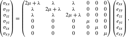
where and are termed Lamé coefficients. The bulk modulus is the ratio of pressure to volume change.

Equation (A2.10) can be expanded as

(A2.10a)

(A2.10b)

(A2.10c)

(A2.10d)

By substituting them into (A2.8) and using (A2.1), the equilibrium equation is expressed as

(A2.11a)

or

(A2.11b)

In the static case, with the gravity and body forces neglected, the equation is rewritten as

(A2.12)

where is just the relative volume change (A2.2). Its divergence is deduced as . By taking the Laplacian, it is obtained that

(A2.13)

that is, the displacement vector satisfies the biharmonic equation in equilibrium.

A2.2 Conversions Between Coordinates

Conversions between the cylindrical polar coordinate and Cartesian coordinate are

The unit vectors are expressed as: , ; and , . Their derivative operations are

(A2.14a)

(A2.14b)

The strains are written as

(A2.15)

The conversions between the two coordinates are

(A2.16a)

(A2.16b)

(A2.16c)

(A2.17a)

(A2.17b)

(A2.17c)

It is derived that the relative transverse area change is . From the related vector operations:

(A2.18)

(A2.19)

the motion equations are written as

(A2.20)

(A2.20b)

(A2.20c)

Hooke's law in the cylindrical polar coordinate for isotropic media is the same as (A2.10) with corresponding subscripts:

(A2.21)

From the conversion between two Cartesian coordinates with angle of θ in (x−y) plane:

(A2.22)

the strain conversions are expressed as

(A2.23a)

(A2.23b)

(A2.23c)

A2.3 Plane Deformation

When it is unnecessary for one of three-dimensional strains or stresses to be taken into consideration, the three-dimensional problem is degraded to a two-dimensional one.

In case 1, with no deformation in z-direction, that is, uz = 0, for example, the medium is bounded by rigid bodies, it is derived that ezz = ezx = ezy = 0 and . The strains to be solved are exx, eyy, exy; the stresses to be solved are with . Hooke's law is expressed as

(A2.24a)

(A2.24b)

(A2.24c)

and

(A2.24d)

The equilibrium equations without body forces are

(A2.25)

Their general solutions take forms of

(A2.26)

where is an arbitrary function of x and Y, satisfying the related boundary conditions, called the stress function. It is seen that

(A2.27)

Therefore, the stress function satisfies the biharmonic equation: . The longitudinal stress is then expressed as .

In case 2, with no stress in z-direction, that is, , for example, no external force in z-direction exists, it is derived that

(A2.28a)

(A2.28b)

(A2.28c)

(A2.28d)

and

(A2.28e)

It is seen that the same equilibrium equations as those of case 1 hold; and a stress function with the same properties exists.

The plane deformation in the polar coordinate is described by the following formulas. Three strain components are considered:

(A2.29)

The equilibrium equations for the isotropic medium without body forces are expressed as

(A2.30a)

(A2.30b)

Hooke's law is expressed as

(A2.31)

The biharmonic equation for the stress function is written as

and the relations between the stresses and the stress function are written as

(A2.32)

A2.4 Equilibrium of Plates and Rods

A2.4.1 The Equilibrium Equation for a Thin Plate

A plate is regarded as a thin plate, if its thickness is much thinner than its transverse size, typically several tenths. Its deformation is regarded as a problem of small deflection, if the displacement occurs only in the direction perpendicular to the plane before deformation, and the strain in the direction is negligibly small, that is, , and . Figure A2.1 shows a section of plate. It is noted that the part on the convex side is stretched, whereas the part on the concave side is compressed; and a neutral surface exists at the middle, on which there is no extension, nor compression.

The equilibrium equation for the thin plate is deduced as

(A2.33)

where is called the flexural rigidity of the plate, P(x, y) is the pressure difference between the two sides. In dynamic states, the motion equation is expressed as

(A2.34)

A2.4.2 Bending of a Rod

For a rod bent in x–z-plane, its strain can be regarded as a plane deformation if the deflection is small enough so that the deformation in y-direction is neglected, that is, with eyy = eyz = eyx = 0. The bending induced stretching and compression cause stains in z-direction:

(A2.35)

where x is measured from the neutral surface, R is the curvature radius of bending, with denoted as the displacement in x-direction. The stress is written as .

Considering a rectangular rod, as shown in Figure A2.2, the moment of the force on the cross section of an infinitesimal element between z and z+dz is written as

(A2.36)

where I = ba3/12 is the moment of inertia about the y-axis. In equilibrium, My(z)−My(z+dz) = Txdz, where Tx is the shear force of the adjacent element applied on the element, i.e., . The sum of the shear forces at the left side and right side of the element accelerates it as . Thus a motion equation is deduced:

(A2.37)

For a circular cross section with radius R, the moment of inertia is . If the rod is not uniform in z-direction, that is, the moment of inertia is a function of z, the motion equation is expressed as

(A2.38)

where fx(z, t) denotes the external distributed force, including gravity.

When a force F is applied at the free end (z = L) of a uniform rod, the displacement along z-direction is then solved as

(A2.39)

In dynamic cases, its motion for a single frequency is described as

(A2.40)

where the wave vector obeys the eigen equation of

(A2.41)

The eigenvalues are solved as and the eigen frequencies are written as .

A2.4.3 Torsion of Rods

Let us inspect a twisted thin rod with its transverse dimension R much smaller than its length, as shown in Figure A2.3. If the twisting rate is small enough to meet condition of , that is, the relative displacement of adjoining transverse sections is small, the torsional deformation is described by only shear strains, with exx = eyy = ezz = 0 and exy = 0; the last expression means that no deformation of its cross section occurs. With relations of and shear strains in z direction are deduced to be and ; the shear stresses and are then obtained.

Consider a solid rod with circular cross section as a simplified case. The moment of twisting force is . The torsional rigidity is defined as

(A2.42)

For a circular tube, .

A2.5 Photoelastic Effect

The dielectric constant of a solid medium is generally a 3 × 3 tensor with six independent components. It will be affected by the strains, expressed as

(A2.43)

where pij are strain-optic coefficients. The coefficients possess symmetric properties, similar to Hooke's law. For isotropic media the effect is expressed as

(A2.44)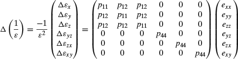

with relation of p44 = (p11−p12)/2. It means that only two coefficients are independent. It can be rewritten as the refractive index change, for example, with shear strains neglected:

(A2.45)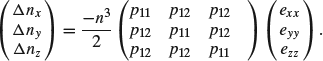

APPENDIX 3: FUNDAMENTALS OF POLARIZATION OPTICS

A3.1 Polarized Light and Jones Vector

A single-frequency planar optical wave propagating in z-direction is expressed generally as

(A3.1)

where E = |E|, , , and . The Jones vector

(A3.2)

is used to describe any polarized light wave, including linear polarized light wave with and the polarization direction α, and circularly polarized light waves with and , where the sign is positive for right circular polarization (RCP) and negative for left circular polarization (LCP). NB: RCP is defined as the rotation of E vector in CW way when viewed towards –z direction; and LCP is in CCW way. Their Jones vectors are written as and .

Figure A3.1 shows the electric field trace in the transverse plane of an elliptically polarized light. From the relation between the two Cartesian coordinates: x∼y and ξ∼ψ, conversions of polarization parameters are deduced as

(A3.3)

(A3.4)

where positive and negative signs correspond to right and left elliptically polarized waves. Jones vector is then converted to in ξ∼ψ coordinate. The ellipticity is expressed as .

A3.2 Stokes Vector and Poincaré Sphere

The Jones vector is a good description of a fully polarized single frequency lightwave. In general cases, the Stokes vector is needed, which has four components, expressed as

(A3.5a)

(A3.5b)

(A3.5c)

(A3.5d)

where stands for the statistic average to take the degree of coherence into consideration. For an elliptically polarized wave, described by Jones vector , Stokes components are simplified as , and , satisfying relation of S21+S22+S23 = S20. It is shown that S0 is the intensity of the optical beam; S1 stands for the wave linearly polarized in x-direction; −S1 stands for the wave linearly polarized in y-direction; stand for the wave linearly polarized in -directions; stand for right and left circularly polarized waves, respectively.

For a partly polarized wave, S21+S22+S23<S20; and for a natural light beam without polarization, S21+S22+S23 = 0. The degree of polarization is defined as

(A3.6)

Poincaré sphere is a sphere in a space with three components of the Stokes vector as its axes, as shown in Figure A3.2. Points in the sphere correspond to the different polarization states: the points on the equator (circle HCVD) stands for a linearly polarized wave; the north and south poles (point R and L) stand for right and left circularly polarized waves, respectively; the north and south halves stand for the right and left elliptically polarized waves, respectively. Points inside the sphere stand for partly polarized waves with DOP<1; the center is for the nonpolarized wave. It is seen for from (A3.3) and (A3.4) that , and , as depicted in the Poincaré sphere.

A3.3 Optics of Anisotropic Media

For the anisotropic media, especially the electro-optic crystals, the dielectric constant is a tensor, expressed as

(A3.7)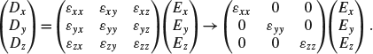

The latter form is the expression in the principal axis coordinate. In general, the direction of vector D is no longer in the direction of electric vector E. Therefore, the direction of the optical wave vector does not coincide with the direction of energy flow, that is, the Poynting vector, since the former is , different from the latter, . On the interface of the anisotropic medium the wave vector refracts according to the condition of phase matching, whereas the optical beam propagates in different directions, which, moreover, depends on its polarization, resulting in the double refraction (birefringence).

Two kinds of anisotropic crystals are found: uniaxial crystals with , and biaxial crystals with different from each other. To understand the properties of the anisotropic media, the index ellipsoid (Optical Indicatrix) is used as a representation of electric impermeability (the inverse tensor of the dielectric constant). In the principal axis coordinate, it is expressed as

(A3.8)

For the uniaxial crystal, n1 = n2 = no, n3 = ne, where the subscripts o and e stand for the ordinary wave and extraordinary wave. They have perpendicular polarizations. For the ordinary wave, D is parallel to E; whereas for the extraordinary wave, they are not parallel.

Based on the birefringence, the medium is used to make a polarizer, a phase retarder, and other optical components. Figure A3.3 shows the optical paths of o-wave and e-wave in a phase retarder, which is also called a wave plate. The phase difference between o-wave and e-wave in normal incidence, passing through the crystal with thickness d, is . The most widely used wave plates are the half wavelength plate with , and the quarter wavelength plate with . It is obvious that the phase retard depends on the wavelength. Therefore, the wave plate has a working linewidth; the smaller the integer m, that is, the thinner the thickness d, the large the linewidth.

A3.4 Jones Matrix and Mueller Matrix

When a beam passes through a device, Jones vector of the output is expressed as J1 = TJ0. Matrix T characterizes the device's action. If the device is lossless, its Jones matrix must be unitary: , that is,

(A3.9)

It is deduced from the relation that |T22| = |T11|, and .

The matrix of a wave plate is expressed in the principal axis coordinate as

(A3.10)

where the fast axis is set as the x-axis. The Jones matrix in the coordinate that is rotated θ to the principal axis of the waveplate is

(A3.11)

For a half wavelength plate, ,

(A3.12)

When a linearly polarized wave E0 = [1, 0]Tinputs, the output is obtained, meaning that the output beam remains a linearly polarized wave, but its polarization is rotated . In case of , the polarization direction coincides with that of the input.

For a quarter wavelength plate, ,

(A3.13)

When the principal axis is -off the input wave, which is polarized linearly on x-axis (or y-axis), we have

(A3.14)

the output will be a circularly polarized wave.

A polarization controller, which convertes the input wave to an output with desired polarizations, can thus be composed by concatenating quarter waveplates and half waves with their relative orientation rotatable.

The Jones matrix of a linear polarization analyzer (polarizer) is expressed as

(A3.15a)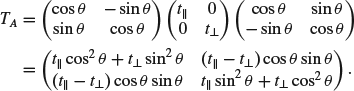

where and are the transmissions of incident beams with polarizations parallel and perpendicular to the axis of analyzer, respectively. For an ideal analyzer with and ,

(A3.15b)

When a wave is denoted by (A3.2) inputs, the output Jones vector is obtained:

(A3.16)

Its power is expressed as

(A3.17)

In case partly polarized waves are involved, the Stokes vector must be used; and the device is characterized by the Mueller matrix: S1 = MS0.

(A3.18)

(A3.19)

(A3.20)

(A3.21)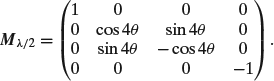

A3.5 Measurement of Jones Vector and Stokes Vector

The polarization characteristics of an optical wave are measured by an instrument composed of a polarizer, an analyzer, and wave plates, as shown in Figure A3.4, where DUT is a device under test.

A3.5.1 Measurement of Jones Vector

The input optical wave is described by . First, powers are measured by using an analyzer in three orientations: , and . The results are I01 = H2, I02 = K2, and . Thus, the parameters of Jones vector are obtained: , and .

To determine the sign of , powers are measured again with a quarter wave plate inserted. The wave behind the wave plate is under condition that the axis of wave plate is aligned coincident with the axis of the analyzer. The measured powers are obtained to be I11 = H2 = I01, I12 = K2 = I02, and . It is obtained that ; or with I0 = I01+I02 = I11+I12.

To reduce the errors of alignments, more measurements are made with , and the measured data are averaged.

A3.5.2 Measurement of Stokes Vector

First, powers of the input wave polarized in x- and y-directions with a polarization analyzer are measured; that is I1 for E1 = PxE0 and I2 for E2 = PyE0. It is then obtained that S0 = I1+I2 and S1 = I1−I2.

Second, powers of the input wave polarized in directions are measured; that is, I3 for E3 = P45E0 and I4 for E4 = P−45E0. From Mueller matrix (A3.20), and . Thus, S2 = I3−I4 is obtained.

Third, let the input pass through a quarter wave plate with . It is transformed to . Powers I5 for E5 = P45E01 and I6 for E6 = P−45E01 are measured with relations of and . S3 = I5−I6 is obtained.

In practice, the loss of polarizer and wave plate should be taken into account. The measurement of Stokes vector is the basis of polarimeter.

APPENDIX 4: SPECIFICATIONS OF RELATED MATERIALS AND DEVICES

Table A4.1 ITU-T Communication Fibers

Table A4.2 Erbium-Doped Fibersa

Table A4.3 PANDA Polarization Maintaining Fibersa

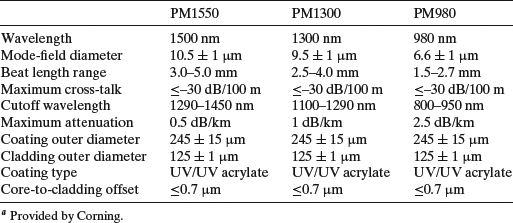
Table A4.4 Typical Parameters and Specifications of LD*

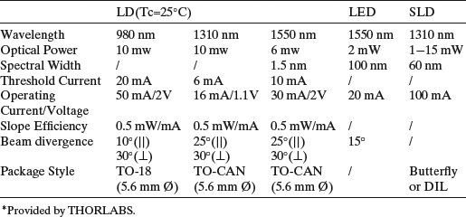
Table A4.5 Typical Parameters and Specifications of PDa

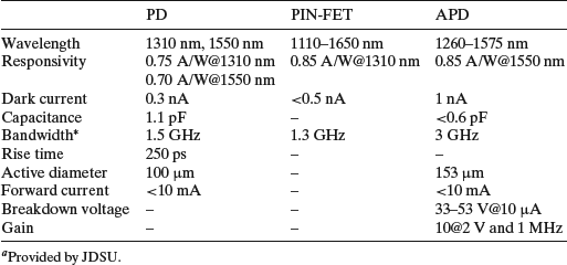
Table A4.6 Main Specifications of LN-MZMa

Specifications	Condition	Specification
Wavelength range		1528–1564 nm
Insertion loss		2.5–5 dB
Return loss	Input an output ports	35 dB
DC Vπ	Differential drive	< 2 V
MZ extinction ratio		25 dB
RF bandwidth		12 GHz
RF voltage	At 2 GHz	< 2.6 V
a JDSU 10 Gb/s double drive MZM.

A4.1 Fiber Connectors

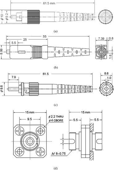
Fiber connectors are used widely in optical communication and fiber sensor systems. The fiber connector fixes the fiber at the middle of a ceramic ferrule, and can be inserted coaxially and precisely into an adapter with a ceramic tube. Most widely used connectors are divided into two types: PC (physical contact) and APC (angled physical contact). PC makes the gap between two end facets of the fibers to be connected as thin as possible to eliminate almost all Fresnel reflection, which would occur at the interface between silica and air. The end surface is polished into a spherical form with its top coincided with the fiber axis, as illustrated in Figure A4.1a. To further reduce the reflection R, the facet is lapped and polished in an angle of ∼8° off the fiber axis, called APC, as shown in Figure A4.1b. In APC connectors, the residual reflected beam will be deflected off the fiber axis to be lost in a short propagation. Two specification items are used to characterize the performance: the insertion loss and the return loss; the latter is defined as

(A4.1)

Figure A4.2 shows the structures of commercial connectors and a typical adaptor used widely today.

The typical insertion loss of FC/PC connection is 0.15 dB for single mode fibers, and 0.3 dB for multimode fibers; and the typical return loss is 50 dB for PC connection, and 65 dB for APC connection.