Chapter 6. Common Mechanisms
In the previous chapter, we introduced the Machinations framework and showed how you can use Machinations diagrams to model the internal economy of games. In this chapter, we introduce some advanced features of the Machinations framework that will permit you to simulate and study more complex economies. We also discuss how feedback structures can be read from a Machinations diagram. As we discussed in Chapter 3, “Complex Systems and the Structure of Emergence,” feedback plays an important role in the creation of emergent behavior, and in this chapter we outline seven important characteristics of feedback structures. Finally, we address ways you can use randomness to add unpredictability and variation to the behavior of your internal economy. This way, Machinations diagrams, both static and digital versions, become an essential tool to help designers understand the nature of the dynamic system of game mechanics that drives the gameplay of their game.
More Machinations Concepts
To start with, we introduce a few additional features of digital Machinations diagrams that we didn’t include in Chapter 5, “Machinations.” In this section, we’ll explain these extra features.
Registers
Sometimes you’ll want to make simple calculations in a Machinations diagram or use numeric values that come from player input. While it is possible to model most of these features with pools, interactive sources, interactive drains, and state connections, the resulting diagram is awkward to read. To simplify things, digital Machinations diagrams offer an additional node type: registers. Registers are represented as solid squares with a number indicating their current value.
In many ways, a register acts just like a pool that always displays its value as a number. A register can be passive or interactive. A passive register has a value that is set by input state connections. When a diagram is not running, this value is displayed as x because it is not yet determined. An interactive register has an initial value that you can set while designing the diagram. In addition, it has two buttons that allow the user to modify its value while the diagram is running. An interactive register is the equivalent of a pool connected to an interactive source and an interactive drain (Figure 6.1).
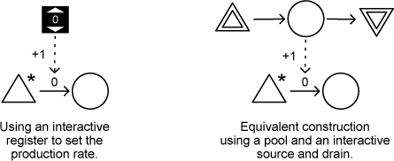
Figure 6.1. An interactive register and its equivalent construction
Registers do not collect resources like pools do, so you should not connect resource connections to a register. You can connect node modifier state connections to registers in the same way you can connect state connections to a pool.
Passive registers allow you to perform more complex calculations. Every state connection that you connect to a register as an input is assigned a letter automatically. You can give the register a formula that uses these letters to determine the value of the register (Figure 6.2). In addition, you can also use the labels max and min to set a passive register to the maximum or minimum value of its inputs.
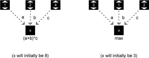
Figure 6.2. Performing calculations using passive registers
Intervals
Sometimes you want a node in a Machinations diagram to be activated less often than every time step. You can accomplish this by creating flow rates with an interval. Intervals are created by using a slash (/) in the flow rate: A source that has an output rate of 1/5 will produce 1 resource every 5 time steps. (See Figure 6.3 for three examples.) A similar effect can be created when the output rate is set to 0.2. However, using intervals allows you more control over the interval and allows you to produce resources in bursts. For example, a production rate of 5/10 would produce 5 resources at once every 10 steps.
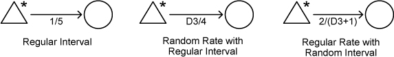
Figure 6.3. Intervals
You can use random flow rates with intervals. A production rate of D6/3 will produce between one and six resources every three steps. Intervals can be random as well. A production rate of 1/(D4+2) indicates that one resource is produced every three to six steps. Random intervals can be a good way to keep the player’s attention on the game (see the “Random Intervals in Games” sidebar). You can even use a production rate of D6/D6, which indicates between one and six resources are produced every one to six steps.
Intervals can also be modified dynamically. Label modifiers that have an i as a unit of their modification (for example, +1i or -3i) will change their target’s interval. For example, in Figure 6.4, the interval of the output of the source A is increased as more resources arrive in pool B.

Figure 6.4. Dynamic intervals
Multipliers
When working with random flow rates, it is often useful to combine multiple chances into one value. For example, a source might have two chances to produce a resource during every time step. You can represent this with two outputs with a probable flow rate for each (Figure 6.5, left side), but as long as the probabilities are equal for each chance, using a multiplier is more convenient. A multiplier is created by adding n* before the flow rate, for example 3*50%, 2*10%, or 3*D3 (Figure 6.5, right side). The two constructions are equivalent, but the one on the right is less cluttered. If you need to use different probabilities, however, you will have to create a construction like the one on the left.
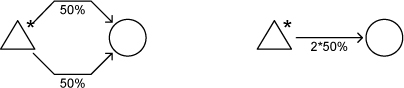
Figure 6.5. Multiplying a flow rate
Like intervals, multipliers can also be modified dynamically. Label modifiers that have an m as a unit of their modification (for example, +2m or -1m) will change their target’s multiplier. For example, the multiplier of the input of the drain A in Figure 6.6 is controlled by the register B. If you run this diagram in the tool and click A (an interactive drain), it will attempt to drain two items from the pool, with a 50% chance of success for each one. If you change the value in the B register, you can raise or lower the number of items that A attempts to drain.
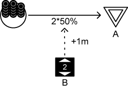
Figure 6.6. A dynamic multiplier
Just like any other label modifier, a label modifier with an m on its own label transmits the change in the source node. Although the value of register B in Figure 6.6 is the same as that on the resource connection, it doesn’t have to be. If the label modifier’s connection were +2m, it would transmit double the change in B.
Delays and Queues
In many games, producing, consuming, and trading resources takes time. The time it requires to complete an action might be crucial for the game balance. In a Machinations diagram, a special node can be used to delay the flow of resources as they travel. A delay is represented as a small circle with an hourglass inside (Figure 6.7).

Figure 6.7. Producing soldiers takes time and resources.
The label on the delay’s output indicates how many time steps a resource is delayed. (Note that this is different from most labels on resource connections, which ordinarily represent a flow rate.) This time is dynamic. Other elements in the diagram can change the delay setting through label modifiers. You can also specify a random delay time using dice notation. A delay can process multiple resources simultaneously. This means that all incoming resources are delayed for the specified number of time steps irrespective of the number of resources currently being delayed.
A delay can also be turned into a queue. A queue has two hourglass symbols instead of one. Queues process only one resource at a time. For Figure 6.8, this would mean that only one resource is passed every five time steps.

Figure 6.8. Building orders are queued and executed one at a time.
Delays and queues can use state connections that communicate the number of resources they are currently processing (including the number of resources waiting in a queue to be processed). This can be useful to create timed effects. For example in Figure 6.9, activating delay A will activate source B for 10 steps. You can activate the delay as long as there are resources on pool C. A construction like this can be used to improve the construction discussed for power pills in Pac-Man in the section “Power Pills” in Chapter 5.
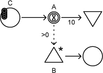
Figure 6.9. Using a delay to create a timed effect
Reverse Triggers
In some games, bad things happen when the player doesn’t have the resources required by an automatic or randomly triggered element. For example, in Civilization when the player runs out of gold to pay the upkeep for his cities’ improvements, the game automatically sells some of them. To simulate this type of event, the Machinations diagrams include a reverse trigger. A reverse trigger is a state connection that is labeled with a !. If its source node tries to pull resources but cannot pull all resources as indicated by the source’s input connections, the reverse trigger will fire its target node. Figure 6.10 illustrates how a reverse trigger can be used to model the automatic sale of city improvements in Civilization.
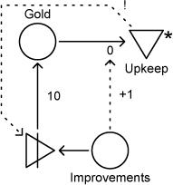
Figure 6.10. Automatic sale of a city improvement when the player runs out of gold in Civilization
Reverse triggers can also be used to trigger end conditions to make a game stop. For example, in Figure 6.11 this construction is used to end a game when a player takes more damage after she has lost all hit points. (In the figure the damage is caused by the user clicking the interactive damage drain. Obviously in most games damage will be caused by triggers produced by other mechanisms.)

Figure 6.11. Ending a game when a player takes damage when she is out of hit points.
Color-Coded Diagrams
Machinations diagrams can include color coding to help you distinguish among different types of resources as they flow around. To create a color-coded diagram in the online tool, simply select the Color-Coded option in the diagram settings dialog in the side panel.
In a color-coded Machinations diagram, the color of resources and connections is meaningful. If a resource connection has a different color than its source, it will pull only resources of its own color. Likewise, if a state connection has a different color from its source, it will respond only to the resources of that color and ignore all other resources. Color-coding allows you to store different resources in the same pool, and for certain games this is very useful. Later in this chapter, we’ll show how color-coding can be used to effectively model different unit types in a strategy game.
If you don’t check the Color-Coded option in the tool, you can still color elements of your diagram for illustration purposes, but the simulation will act as if everything is all the same color.
In a color-coded diagram, one source or converter can produce different colored resources if its outputs are of a different color than the source or converter itself. Gates can use different colored outputs to sort resources of different colors.
Figure 6.12 illustrates how color coding can be used. In this figure, source A produces a random number of orange and blue resources every time it is activated. Both are collected at pool B. The number of orange resources in B increases the number of blue resources produced at A, and vice versa. The user can activate drain C only when there are at least 20 orange and 20 blue resources in pool B.
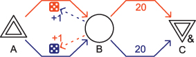
Figure 6.12. A color-coded diagram
In a color-coded diagram, a gate can be used to change the colors of resources that pass it. If the gate has color-coded outputs, it will try to sort resources by their color, sending red resources along a red output, and so on. However, if the incoming resource color doesn’t match any of the outputs, the gate selects an appropriate output (based on random numbers if it is a random gate or spreading the resources according to the weighting of the outputs if it is a deterministic gate) and changes the resource to that color. For example, Figure 6.13 uses this construction to randomly produce red and blue resources with an average proportion of 7/2.
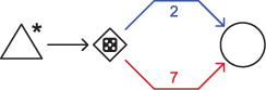
Figure 6.13. Producing resources with random colors
Delays and queues can use color coding. By giving them outputs with different colors, they will delay resources of the corresponding color by a number of time steps indicated by that output. For example, Figure 6.14 represents the mechanics of a game where players can build knights and soldiers. Knights are represented as red resources, and soldiers are represented as blue resources. Knights cost more gold and take more time to build.
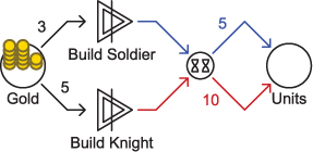
Figure 6.14. Using color coding to build different units with one building queue
Feedback Structures in Games
The structure of a game’s internal economy plays an important role in a game’s dynamic behavior and gameplay. In this structure, feedback loops play a special role. A classic example of feedback in games can be found in Monopoly where the money spent to buy property is returned with a profit because more property will generate more income. This feedback loop can be easily read from the Machinations diagram of Monopoly (Figure 6.15): It is formed by the closed circuit of resource and state connections between the Money and Property pools.
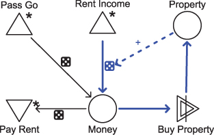
Figure 6.15. Monopoly
Closed Circuits Create Feedback
A feedback loop in a Machinations diagram is created by a closed circuit of connections. Remember that feedback occurs when state changes create effects that ultimately feed back to the original element. A closed circuit of connections will cause this effect.
A closed circuit of only resource connections (as in Figure 6.16) cannot display very complex behavior. The resource is pulled through the pools in circles creating a simple periodic system, but nothing more interesting can happen.
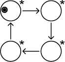
Figure 6.16. Feedback created by only resource connections. The resource simply goes round and round.
The most interesting feedback loops consist of a closed circuit that mixes resource connections and state connections. The loop should contain at least one label modifier or activator. For example, the mechanism in Figure 6.17 uses an activator to maintain the resources in the pool at about 20. It acts the way a heating system does to keep a room warm in cold climates: It turns on a heater with a fixed output when the temperature drops below 20. The graph in the same figure displays the temperature over time.
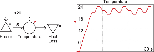
Figure 6.17. Heater feedback mechanism using an activator
You can build a similar system using a label modifier instead (Figure 6.18). In this case, the heater’s output rate is adjusted by the actual temperature, creating a more subtle temperature curve. This simulates a heater that can produce varying amounts of heat rather than a fixed amount, as in Figure 6.17.

Figure 6.18. Heater feedback mechanism using a label modifier
Feedback by Affecting Outputs
A feedback loop can also be created by a circuit of connections that affects the output of an element. For example, consider a Machinations diagram for an air conditioner (Figure 6.19). The higher the temperature, the faster the temperature is drained.
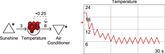
Figure 6.19. An air conditioner in Machinations
Any changes that affect the output of a node can also close a feedback loop. In this case, output can be affected directly by a label modifier or by a trigger or activator affecting an element at the end of the resource that is able to pull resources (such as a drain, converter, or gate, as in Figure 6.20).
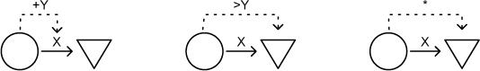
Figure 6.20. Closing a feedback loop by affecting the output
Positive and Negative Feedback Basketball
In Chapter 4, we briefly introduced Marc LeBlanc’s concept of positive and negative feedback basketball to explain the effects of positive and negative feedback on games. In this section, we’ll discuss the idea in more detail and show how to model it in Machinations.
Positive feedback basketball is played like normal basketball but with the following extra rule: “For every N points of difference in the score, the team that is ahead may have an extra player in play.” Figure 6.21 shows a model of positive feedback basketball. It uses a very simple construction to model basketball itself: Every player on a team has a particular chance to score every time step. Teams initially consist of five players, so their chance to score is represented as a source with an initial production rate of five (for simplicity, we assume that a basket is worth one point, not two, and we ignore three-point shots and free throws). Next comes a gate with a percentage; this indicates the percentage of player attempts that actually succeed in scoring. As you can see, the blue team is much better than the red team is; the blue team’s chance of scoring is 40% while the red team’s chance is only 20%. A pool called Difference keeps track of the difference in the points scored, because every time blue scores, a point is added to the Difference pool, and every time red scores, a point is subtracted. Each team can field one more player for every five points that it leads by—if it’s ahead by five, it gets one more player; if it’s ahead by 10, it gets two; and so on. The development of the scores and the difference in the scores are plotted over time in the chart. As you can see, the score of the better team quickly spirals upward as the difference increases, allowing them to field more and more players.
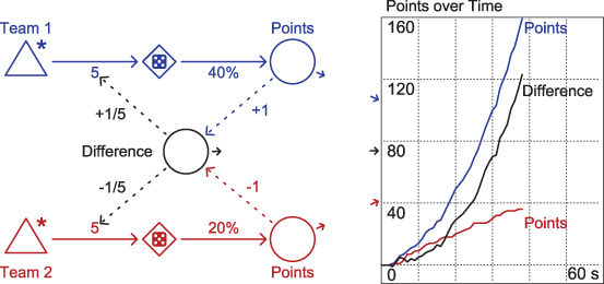
Figure 6.21. Positive feedback basketball. Team sizes are prevented from dropping below 5 by setting their minimal value to 5.
In negative feedback basketball, the extra rule is reversed: The losing, rather than the leading, team can field an extra player for every N points of difference. Again, this can be easily modeled as a Machinations diagram, simply by reversing the signs of a few state connections. The chart that is produced by running the diagram is harder to predict. Without looking at Figure 6.22, can you guess what happens to the points of both teams and the difference in scores?
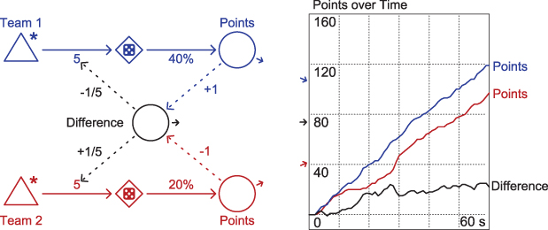
Figure 6.22. Negative feedback basketball
The chart in Figure 6.22 surprised us when we first produced it. Where you might expect the negative feedback to cause the poorer team to get ahead of the better team, it never does. What happens is that the negative feedback stabilizes the difference between the two teams. At some point, the poorer team is so far behind that their lack of skill is compensated for by their team size, and beyond this point, the difference doesn’t change much.
Another interesting effect of feedback occurs when you have two teams of similar skill play positive feedback basketball. In that case, both teams will score at a more or less equal rate. However, once one of the teams by chance takes a lead, the positive feedback kicks in, and they can field more and more players. The result might look something like Figure 6.23.
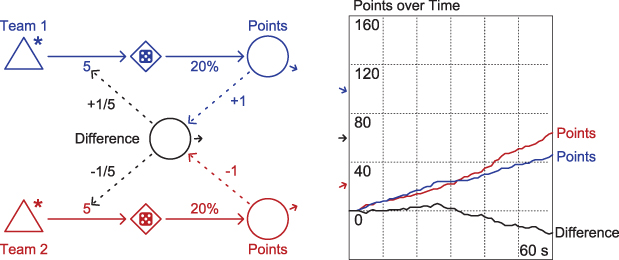
Figure 6.23. Positive feedback basketball between two equal teams. Notice the distinctive slope in the line that depicts the difference between the scores after roughly 30 steps.
Multiple Feedback Loops
In the section “Categorizing Emergence” in Chapter 3, we discussed Jochen Fromm’s typology of emergent systems. According to Fromm, systems with multiple feedback loops display more emergent behavior than systems with only one feedback loop. This is also true for games. Most games need more than one feedback loop to provide interesting emergent behavior. The board game Risk is an excellent example of this. In Risk, no fewer than four feedback loops interact.
Like Monopoly, Risk is a classic board game that illustrates certain principles of mechanics design well. If you are not familiar with Risk, you can download a copy of the rules at www.hasbro.com/common/instruct/risk.pdf. The Wikipedia entry for Risk also includes an extensive analysis.
The core feedback loop in Risk involves the resources armies and territories: The more territories a player holds, the more armies he can build. Figure 6.24 depicts this core feedback loop. The player expends armies to gain territories by clicking the interactive Attack gate. The armies that succeed pass to the converter, which turns them into territories. The label +1/3 of the label modifier that sets the output flow rate of the interactive source Build indicates that the output of the source goes up by one for every three territories the player has.
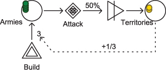
Figure 6.24. The core feedback loop involving armies and territories in Risk
In the real game, not every trio of cards generates armies, and some trios generate more armies than others. We have simplified this by making the exchange rate of cards for armies random. In Figure 6.25, this is indicated by the die symbol labeling the output of the Trade Cards converter.
When a player gains a territory, he receives a card. These may be collected into sets and exchanged for more armies. The second feedback loop in Risk is formed by the cards that are gained from a successful attack (Figure 6.25). Only one card can be gained every turn, so the flow of cards passes through a limiter gate first. Collecting a set of three cards can be used to generate new armies. The interactive converter Trade Cards changes three cards into a random number of armies.
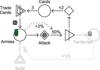
Figure 6.25. The second feedback loop in Risk, involving cards and armies
The third feedback loop is activated when a player manages to capture an entire continent, which will give the player bonus armies every turn (Figure 6.26). In Risk, predefined groups of territories form continents as indicated by the design of the game board. In the diagram, this level of detail is not possible, so instead the construction is represented as a pool connected to another pool with a node modifier. In this particular case, five territories count as one continent, which will in turn activate the bonus source.

Figure 6.26. The third feedback loop in Risk: bonus armies through the possession of continents
Finally, the fourth feedback loop is activated by the loss of territories because of the actions of other players. Which player chooses to attack which other player depends on many factors, including the attacker’s position, strategy, and preferences. Sometimes it makes sense to prey on weaker players in order to gain territories or cards, and sometimes it is important to oppose stronger players to keep them from winning. The number of continents a player holds has a strong influence on this. Because continents generate bonus armies, players will generally attack aggressively to prevent others from keeping a continent (Figure 6.27). The important thing is that in Risk there is some form of friction caused by other players, and the influence of this friction increases when the player has captured continents. This type of friction is a good example of the negative feedback that can almost always be found in multiplayer games where players can act against each other, especially if they are allowed to collude against the lead player.
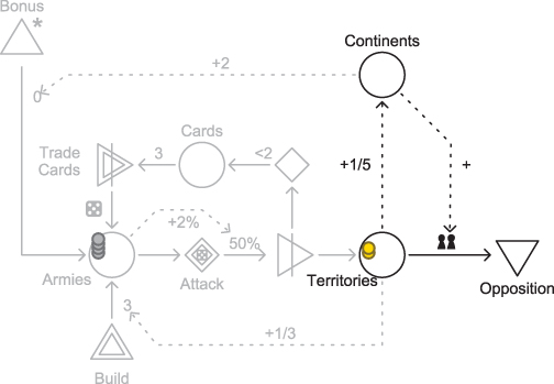
Figure 6.27. The fourth feedback loop in Risk: Capturing continents provokes increased attacks by other players.
In the diagram, the loss of territories taken by other players’ attacks is indicated by the multiplayer dynamic label (an icon depicting two pawns) affecting the resource flow to the Opposition drain. See Table 6.2 for more information about this and other types of nondeterministic behavior.
Figure 6.28 shows the entire Risk diagram. It does not model the entire game exactly; like our Pac-Man example in Chapter 5, this is an approximation. See the “Level of Detail” sidebar.
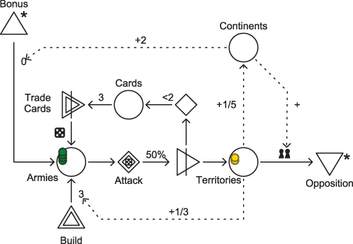
Figure 6.28. The complete Risk diagram
Feedback Profiles
The first three feedback loops in Risk all are positive: More territories or cards lead to more armies, which lead to more territories and cards. Yet they are not the same: They have different profiles. The feedback of capturing territories to be able to build more armies is straightforward, is fairly slow, and involves a considerable investment of armies. Often players lose more armies in an attempt to conquer territories than they regain with one build. This leads to the common strategy to build during multiple, consecutive turns. The feedback of cards is much slower than the feedback of territories. A player can get only one card each turn, and she needs at least three to create a complete set. At the same time, the feedback of the cards is also much stronger: A player might get between four and ten armies depending on the set she collects. Feedback from capturing continents operates faster and more strongly still, because it generates bonus armies every turn. This feedback is so strong and obvious that it typically inspires fierce countermeasures from other players.
These properties are important characteristics of the feedback loops that have a big impact on the dynamics of the game. Players are more willing to risk an attack when it is likely that the next card they will get completes a valuable set: It does not improve their chances of winning a battle, but it will increase the reward if they do. Likewise, the chance of capturing a continent can inspire a player to take more risk than the player should. In Risk the player’s risks and rewards constantly shift, making the ability to understand these dynamics and to read the game a critical skill. These three positive feedback loops play an important role, but simply classifying them as positive does not do justice to the subtlety of the mechanics. It is important to understand how quickly and how strongly each operates.
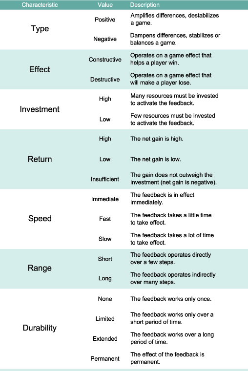
Seven Feedback Characteristics
Table 6.1 lists seven characteristics that, together with the determinability characteristic discussed next, form a more detailed profile of a feedback loop. At first glance, some of these characteristics might seem as if they overlap, but they do not. It is easy to confuse positive feedback with constructive feedback and negative feedback with destructive feedback. However, positive destructive feedback does exist. For example, losing pieces in a game of chess will increase the chance of losing more pieces and losing the game. Likewise, in Civilization, the growth of a city is slowed down by the corruption that is caused by large cities: negative feedback on a constructive effect.
Table 6.1. Seven Characteristics of Feedback
The strength of a feedback loop is an informal indication of its impact on the game. Strength cannot be attributed to a single characteristic; it is created by the interactions of several. For example, permanent feedback with a little return can have a strong effect on the game.
Changes to the characteristics of a game’s feedback loops can have a dramatic effect on the game. Feedback that is indirect and slow but with a lot of return and not durable has a strong destabilizing effect. In this way, even negative feedback can be used to destabilize a system if it is applied erratically or when its effects are strong but slow and indirect. It means that at a much later point in the game something big will happen that is difficult to predict or prevent.
The profile of feedback created by direct interaction in a multiplayer game, such as the ability to target specific players for an attack in Risk, can change depending on the players’ strategies. Feedback from direct interaction often is negative and destructive: Players act against, or even conspire against, the leader. At the same time, it can turn into positive and destructive feedback when someone starts to prey on the weaker players.
Feedback characteristics can be read from a Machinations diagram, although this is easier for some characteristics than it is for others. In general, use the following guidelines:
• To determine a feedback loop’s effect, look at how it is connected to different end conditions. If the feedback mechanism is directly connected to a winning condition, it is probably constructive; if it is directly connected to a losing condition, it is probably destructive.
• A feedback loop’s investment can be determined by looking at how many resources are consumed to activate the mechanism. In addition, feedback mechanisms that require players to activate many elements usually have a high investment, as these mechanisms generally require more time or turns to activate.
• A feedback loop’s return can be determined by looking at how many resources are produced by the mechanism. Return must be compared to investment to paint a complete picture.
• The speed of a feedback loop is determined by the number of actions and elements involved to activate the feedback loop. Feedback loops that contain delays and queues are obviously slower than those loops that do not include these elements. Feedback loops that involve only automatic nodes tend to be faster than feedback loops that include many interactive nodes. Likewise, in most cases, feedback loops that consist of mostly state connections tend to be faster than feedback loops that consist of mostly resource connections.
• The range of a feedback loop is easily determined by the number of elements it consists of. Feedback loops that consist of many elements have a high range.
• Most feedback loops are fundamental parts of their game’s economy, so their durability is extended or permanent. To identify a feedback loop with limited durability, see whether any part of the loop depends on limited resources that can never be recovered or are recovered only at long intervals.
• The feedback loop’s type is probably the trickiest characteristic to determine simply by looking at a Machinations diagram. Positive label modifiers affecting the flow of production mechanisms create positive feedback, but positive label modifiers affecting the flow toward a drain or a converter tend to create negative feedback. The type of feedback is much harder to determine when the feedback loop involves activators. To determine the type of a feedback mechanism, you must really consider the entire mechanism and all its details.
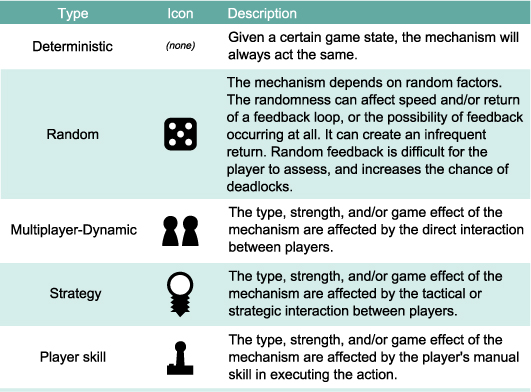
Determinability
In many games, the strength of a feedback loop is affected by factors such as chance, player skill, and the actions of other players. Machinations diagrams represent these factors by different symbols that stand for nondeterministic mechanisms. Table 6.2 lists the symbols used to indicate different types of nondeterministic behaviors. You can use these icons to annotate connections and gates in a diagram. A single feedback loop can be affected by multiple and different types of nondeterministic resource connections or gates. For example, the feedback through cards in Risk (Figure 6.25) is affected by a random gate and a random flow, increasing its unpredictability. The loss of territories is affected by a multiplayer dynamic, namely, attacks by other players.
Table 6.2. Types of Determinability
The skill of a player in performing a particular task can also be a decisive factor in the nature of feedback, as is the case in many computer games. For example, Tetris gets more difficult as the blocks pile up, and the rate at which players can get rid of the blocks is determined by their skill. Figure 6.29 shows this as an interactive gate that controls a converter. Skillful players will be able to keep up with the game much longer than players with less skill. Here player skill is a factor on the operational or tactical level of the game. In games of chance, tactics, or games that involve only deterministic feedback, a whole set of strategic skills can be quite decisive for the outcome. This feedback loop in Tetris is also affected by randomness. The shape of the block is randomly determined by the game. Although the skill is generally more decisive in Tetris, the player just might get lucky.
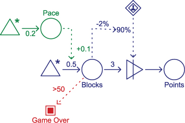
Figure 6.29. Tetris
Randomness vs. Emergence
Games with many random factors become hard, if not impossible, to predict. In games that have too many random factors, players often feel that their actions have little impact on the game. One of the strengths of creating games with emergent gameplay is that most of the dynamic behavior of the game arises from the complexity of the systems, not from the number of dice rolled.
It is our conviction that a well-designed game relies on pure chance only sparingly. A game with only a few deterministic feedback loops can show surprisingly dynamic behavior. When you use emergence rather than randomness to create dynamic gameplay with uncertain outcomes, all decisions made by the player will matter. This encourages her to pay attention and engage with the game.
There are two situations in which adding randomness is a useful design strategy: It can force players to improvise, and it can help counter dominant strategies.
Use Randomness to Force Improvisation
Many games use randomness to create a situation in which the player is forced to improvise. For example, the random maps generated for games such as Civilization and SimCity create new and unique sets of challenges each time players start a new game. In the collectible trading card game Magic: The Gathering, each player builds his own deck by selecting 40 or so cards from his collection. But every time he starts a new game, he needs to shuffle them. Players might control the cards in the deck, but they must deal with them in a random order. Planning and building your deck is one part of the skill that goes into playing Magic: The Gathering. Improvising and spotting opportunities as they occur while the game develops is another.
Improvisation works very well in a game that offers a random but level playing field for all players. If a game generates random events that affect all players equally, the decisive factor in dealing with the events comes from the players’ reaction to and preparation for these events. Many modern, European-style board games tend to use randomness in this way.
Randomness vs. Emergence in Modern Board Games
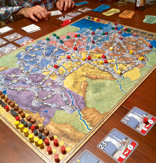
Figure 6.30. Power Grid, German edition. Image courtesy of Jason Lander under a Creative Commons (CC BY 2.0) attribution license.
Use Randomness to Counter Dominant Strategies
A dominant strategy is a course of action that is always the best one available to a player in all circumstances. (It doesn’t guarantee that the player will win; it’s just his best option.) As a designer, it is essential to avoid setting up mechanics that establish a dominant strategy. Games with a dominant strategy aren’t any fun to play, because the players end up doing the same thing over and over again. If you have a dominant strategy in your game, you need to balance your mechanics better (which we’ll discuss in Chapter 8). Sometimes this is too difficult or too time-consuming. In that case, adding more randomness to the mechanism can be an easy way out.
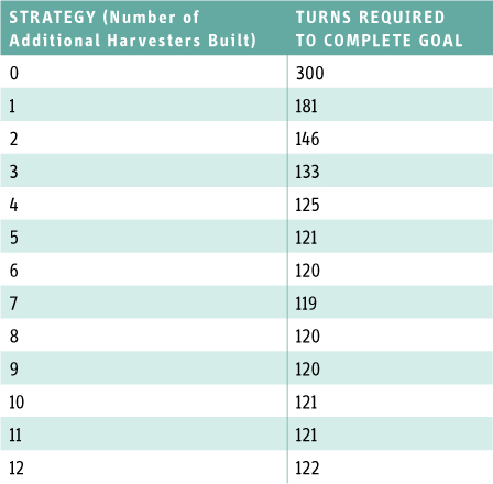
For example, consider the following simple two-player, energy-harvesting game. Each player starts with a harvester that collects 0.1 energy every turn. Players can buy an additional harvester by spending three energy, which increases their harvesting rate. The goal is to collect 30 energy, and whoever collects it first wins. In Figure 6.31, two players (red and blue) are playing. Red’s strategy is to spend all energy to build seven new harvesters before starting to collect energy. Blue’s strategy is to build two new harvesters before collecting.
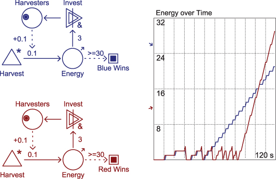
Figure 6.31. A simple deterministic harvester game. Red wins all the time.
Because this game is completely deterministic, the outcome is always the same: Red wins every time. With her strategy, it will take her 119 turns to collect 30 energy, while it will take blue, with his strategy, 146 turns to collect 30 energy. In fact, if we use a Machinations diagram to determine the time it takes to collect 30 energy for all possible options to build between 0 and 11 harvesters, it should become clear that building 7 extra harvesters is the dominant strategy: It simply allows the player to get to the goal the fastest (Table 6.3).
Table 6.3. Comparison of the Different Strategies in the Deterministic Harvesting Game
You might recognize the pattern in the chart from the section “Long-term investments vs. short-term gains” in Chapter 4. It’s the same phenomenon.
Randomness can be used to break this pattern. If the same game were played but instead of harvesting 0.1 energy every turn, a harvester would increase the chance that energy is harvested by 10%, the results completely change. Figure 6.32 shows a sample run of the harvesting game set up in this way. From simulating and running this game 1,000 times, we determined that now blue has roughly a 15% chance to win.
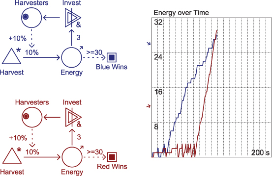
Figure 6.32. The random harvester game. Now blue has a 15% chance to win.
Example Mechanics
In this section, we’ll discuss some mechanics commonly found in games across different genres. We’ll use Machinations diagrams to show how these mechanics can be modeled, but we’ll also use the diagrams to discuss the mechanisms themselves in more detail. You can also find digital versions of all these examples online.
When reading through the example mechanics, you will notice that we often isolate and model different mechanisms individually. This is done partly because models of complete games grow complex very quickly. It would be difficult to grasp all these mechanics from a single diagram for a game, especially because the printed diagrams in the book are static. In many cases, it is simply not necessary to look at all the mechanics in a game to understand the most important ones. After all, games are often built from several dynamic components. Thoroughly understanding each component is the first and most important step toward understanding the dynamic behavior of a game as a whole, even when (as in most games of emergence) the whole is definitely more than the sum of its parts.
Power-Ups and Collectibles in Action Games
The gameplay of action games emerges primarily from interesting physics and good player interaction. The levels of many action games are fairly linear: The player simply needs to perform a number of tasks, each with a certain chance to fail. His objective is to reach the end of a level before running out of lives. Figure 6.33 represents a small level for an action game with three tasks (A, B, and C). Each is represented by a skill gate that generates a number between 1 and 100. The player is represented by a resource that moves from pool to pool. If the player fails to perform a task, there are two options: Either he dies (as is the case with tasks A and C) or he is sent back to a previous location in the level (as is the case with task B).
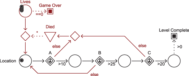
Figure 6.33. Level progression in an action game
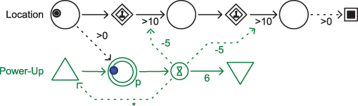
Most action games are more than just a series of tasks, however. They usually have an internal economy that revolves around power-ups and collectible items. For example, in Super Mario Bros., the player can collect coins to gain extra points and lives, while power-ups grant the player special powers, some of which have a limited duration. Power-ups and collectibles can be represented in Machinations diagrams by resources that are harvested from certain locations. Figure 6.34 shows how this might be modeled using different colored resources to indicate different power-ups or collectibles. In this diagram, the player must be present at a certain location to be able to collect the power-up. This diagram also shows how power-ups and collectibles can be used to offer players different strategic options. In this case, the player can progress through the level quickly and fairly easily if she goes from location I to II and V immediately. However, she can also opt for the more dangerous route through III and IV, in which case she can collect one red and two extra yellow resources.
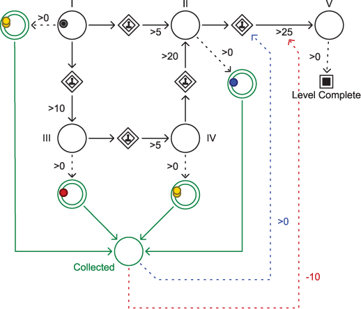
Figure 6.34. Collecting power-ups from different locations in an action game (lives are omitted from this diagram)
In Figure 6.34, the blue power-up and the task that requires it constitute an example of a lock-and-key mechanism. Lock-and-key mechanisms are the most important mechanisms that games of progression use to control how a player progresses through a level. Lock-and-key mechanisms rarely incorporate feedback loops and so seldom exhibit emergent behavior. We will examine lock and key mechanisms in more detail in Chapter 10, “Integrating Level Design and Mechanics.”
Power-ups might be needed to progress through a game, and in that case, finding the right power-ups is a requirement to complete a level. Other power-ups might not be needed but are helpful all the same; in this case, the player must decide how much risk she will take to collect one and how much she stands to gain from it. For example, in Figure 6.34, the blue power-up is required to perform the final task to complete the level, while the red power-up makes that task a little easier.
Collectibles also offer a player a strategic option. For example, if the player must risk lives to collect coins and must collect coins to gain lives, the balance between the effort and risk the player takes and the number of coins to be collected is crucial. In this case, if a player has collected nearly enough coins to gain an extra life, taking more risk becomes a viable strategy. Figure 6.36 represents this mechanism. Note that it forms a feedback loop. In this case, the feedback is positive, but the player’s skill determines whether the return on the investment is enough to balance the risk she takes.
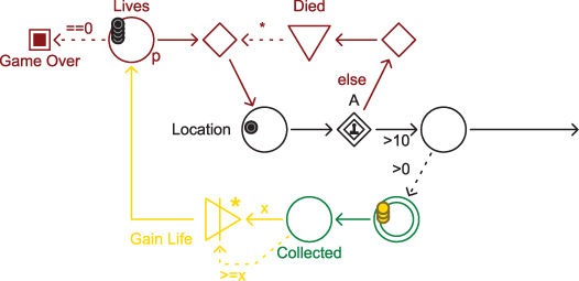
Figure 6.36. Feedback in collecting coins that gain new lives
Racing Games and Rubber Banding
Racing games can be easily framed in economic terms as a game where the player’s objective is to “produce” distance. The first player to collect enough distance wins the game. Figure 6.37 illustrates this mechanism. Depending on the implementation, the production mechanism might be influenced by chance, skill, strategy, the quality of the player’s vehicle, or any combination of these factors. The Game of Goose is an example of a racing game in which chance exclusively determines the outcome of the game. Most arcade racing video games rely heavily on skill to determine a winner. More representative racing games that include vehicle tuning will probably involve some long-term strategy as well.
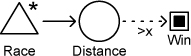
Figure 6.37. Racing mechanism
A simple racing mechanism as represented in Figure 6.37 has a huge disadvantage. If skill or strategy is the decisive factor, the outcome of the game will nearly always be the same. Consider the mechanisms in Figure 6.38. It shows two players racing, and their skill is represented by different chances to produce distance. The chart displays a typical game session and indicates spreads of possible outcome. Obviously, the blue player is going to win nearly all the time.
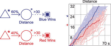
Figure 6.38. An unequal race
We have intentionally implemented an extreme form of rubber banding to make it more visible. Real games would use more subtle boosting.
Many racing games use a technique called rubber banding to counter this effect. Rubber banding is a technique of applying negative constructive feedback based on the distance between the player and his artificial opponents in order to make sure that they stay close. We have seen a construction like this already with LeBlanc’s example of negative feedback basketball. In that discussion, we pointed out that while negative feedback used like this might keep the players close together, it will not really make a poorer player win more often. However, there are adjustments that can be made to the rubber-banding mechanism to change that. If the negative feedback is made stronger and lasts for a time, its effects are changed. Figure 6.39 represents this type of rubber banding. The blue player has a skill level of 60%, while the red player has a skill level of 40%, so blue generates distance more quickly than red. The register at the right computes the difference in distance and, depending on which one is ahead, will signal their Boost source to generate a boost. The boost lasts for 20 time steps, and each boost will improve the player’s performance by 5%. The chart displays a typical game session that results from this mechanism. Note that the chart shows a race in which red and blue take the lead alternately.
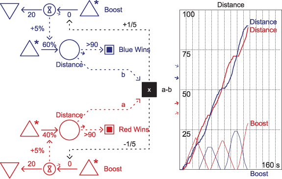
Figure 6.39. Rubber banding with strong and durable negative feedback
RPG Elements
Many games allow players to build up and customize the attributes of their avatars or of a party of characters. Often the mechanics involved are referred to as RPG elements of the game. In this economy, skills and other attributes of player characters are important resources that affect their ability to perform particular tasks. The most important structure of the RPG economy is a positive feedback loop: Player characters must perform tasks successfully to increase their abilities, which in turn increases their chance to perform more tasks successfully.
In classic role-playing games, experience points and character levels act as separate resources that structure the economy. Figure 6.40 shows how these mechanics might be modeled for a typical fantasy role-playing game. In this case, the player can perform three different actions: combat, magic, and stealth. Successfully executing these actions will produce experience points. When a player has collected 10 experience points, he can level up. The experience points are converted into a higher character level and two upgrades that he can use to increase his abilities. (In some games, experience points are not consumed, but trigger upgrades at stated thresholds. You can do this with a source that produces upgrades and an activator to fire it.) To spice up things a little, this diagram also contains a construction that occasionally increases the difficulty of the tasks. Using color-coding, the difficulty of each different task progresses differently. Normally a dungeon master (in the case of a tabletop role-playing game) or the game system would make sure players are presented with suitable tasks.
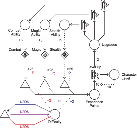
Figure 6.40. RPG economy with experience points and levels
In Figure 6.40, the positive feedback loop is countered partially by a negative feedback loop that is created by increasing the number of experience points required to reach the next level every time the player levels up. This is a common design feature in the internal economies of many role-playing games. Such a structure strongly favors specialization: As players need more and more experience points to level up, they will favor the task they are better at, because these tasks will have a bigger chance to produce new experience points. This can be countered by applying negative feedback to the upgrade cost or impact for each ability separately (Figure 6.41), either instead of, or in addition to, the increasing costs to level up.
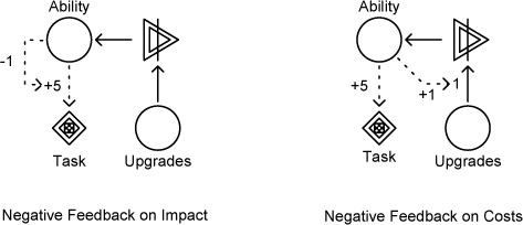
Figure 6.41. Alternative ways of applying negative feedback in an RPG economy
Some RPG economies work differently; they give experience points whether an action succeeds or not. For example, in The Elder Scrolls series, performing an action often increases the player character’s ability, even if that action is unsuccessful. In The Elder Scrolls, negative feedback is applied by requiring the action to be performed more times in order to advance to the next level of ability. This type of mechanism is illustrated in Figure 6.42.
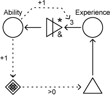
Figure 6.42. An RPG economy without experience points controlled by the player
FPS Economy
At the heart of the economy of most first-person shooters there is a direct relationship between fighting aggressively (thus consuming ammo) and losing health. To compensate for this, enemies might drop ammo and health pick-ups when they are killed. We’ll show how to model this structure in a Machinations diagram in two steps (Figure 6.43 and Figure 6.44).
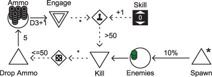
Figure 6.43. Ammunition and enemies in an FPS game
In the first step, ammunition is represented by a pool of resources. When the player chooses to engage an enemy, he wastes between two and four ammunition units and has a chance to kill an enemy. This is modeled by the skill gate between the Engage and Kill drains. In this case, the skill gate is set to generate a random number between 1 and 100 every time it fires. If the generated value is larger than 50, the Kill drain is activated, and one enemy is removed. The register labeled Skill can be used to increase or decrease this chance; it can be used to reflect more or less skilled players. Once an enemy is killed, a similar construction is used to create a 50% chance that five more ammunition resources are generated by the Drop Ammo source, which go into the Ammo pool. To keep things interesting, new enemies are spawned occasionally.
Figure 6.44 adds player health to the diagram. In this case, poor performance by the player when engaging an enemy (such as when a number below 75 is generated by the skill gate) activates a drain on the player’s health. In addition to dropping ammunition, there now is also a 20% chance a killed enemy drops a medical kit (medkit) that the player can use to restore health.
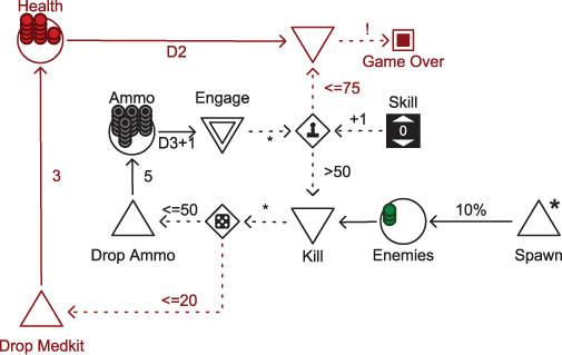
Figure 6.44. Health added to the FPS game economy. Skill gates and random gates generate numbers between 1 and 100.
Analyzing the mechanics in Figure 6.44 reveals that in the basic FPS game economy there are two related positive feedback loops. However, the effectiveness of the return of each feedback loop depends on the skill of the player. A highly skilled player will waste less ammunition, lose less health, and gain ammunition from engaging enemies, whereas a poorly skilled player might be better off avoiding enemies. The amount of ammunition a player needs to kill an enemy and the chance that killed enemies drop new ammunition or medkits obviously is vital for this balance.
You could add a number of additional feedback loops to make this basic game economy more complex. For example, the number of enemies might increase the difficulty of killing enemies or increase the chance players will lose health fighting them, thus creating positive destructive feedback (a downward spiral). Negative constructive feedback could be created by having the player’s ammunition level negatively impact the player’s chance of killing an enemy. Players with little ammunition would magically fight a bit better, while those with a lot wouldn’t fight quite so well. This would tend to damp down the effect of large fluctuations in ammunition availability.
RTS Harvesting
In a real-time strategy game, you typically build workers to harvest resources. Figure 6.45 represents a simple version of this mechanism with only one resource: gold. In this case, gold is a limited resource. Instead of using a source, the available gold is represented with a pool named Mine that starts with 100 resources. Note that the pool is made automatic so that it starts pushing gold toward the player’s inventory (the pool named Gold). The flow rate is determined by the number of workers the player has. Building workers costs two gold units. Note that the converter to build workers pulls gold only when there are two gold available: It is in “pull all” mode as indicated by the & sign.
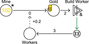
Figure 6.45. Mining for gold in an RTS
Most real-time strategy games have multiple resources to harvest, forcing players to assign different tasks to their workers. Figure 6.46 expands upon the previous one to include a second resource: timber. In this diagram, players can move workers between two locations by activating the two pools representing those locations. Workers in each location contribute to the harvesting of one of the resources. In this case, timber is also a limited resource (the Forest pool). The initial harvesting rate for timber is slightly higher than the harvesting rate for gold. However, as the workers clear the forest, the harvesting rate drops because they have to travel longer distances (you might recognize this situation from Warcraft). This mechanism is modeled by applying a little negative feedback on the harvesting rate of timber based on the number of resources left in the forest.
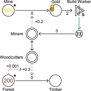
Figure 6.46. Mining gold and harvesting timber
RTS Building
In real-time strategy games, all those resources are harvested for a reason: You need them to build your base and military units. Figure 6.47 illustrates how resources can be used to construct a number of buildings and units. The diagram uses color-coding, and each unit type has its own color. Soldiers are blue, and archers are purple. Building types have their own color too: Barracks are blue, the mill is purple, and towers are red. Different colored activators are used to create dependencies between the building options: You need a barracks to be able to build units and a mill to produce archers and towers.
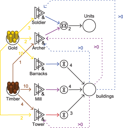
Figure 6.47. RTS building mechanics
RTS Fighting
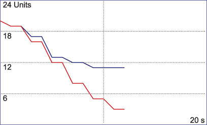
An efficient way of modeling mechanics for combat between units is to give every unit a chance to destroy one unit of the opposition in each time step. This is best implemented with a multiplier. Figure 6.48 illustrates this mechanism. It features generic units from two armies (red versus blue), each in a pool; blue has 20 units, and red has 30. Every unit has a 50% chance of destroying an enemy unit in each time step. This is implemented with a state connection from the pool (the dotted line marked +1m) that controls how many units the blue army will try to drain from the red army, and vice versa. As blue has 20 units at the beginning of the run, the resource connection between the red pool, and its drain reads 20*50%—that is, the 20 blue units each have a 50% chance of killing (draining) a red unit. Similarly, the 30 red units each have a 50% chance of killing a blue unit. In the first time step, the calculation will run, and some number of each armies units will be drained. The state connection will then update the flow rate of the resource connection to reflect the new number of units in each pool.
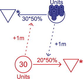
Figure 6.48. Basic combat in a real-time strategy game
Remember that a state connection always tracks changes in the node that is its origin. In Figure 6.48, the state connections reduce the multipliers that they point to because their origin pools are being drained.
We can expand this basic combat construction in two ways. First, we can take into account different unit types by using color coding. For example, we might distinguish between stronger and weaker offensive units by having each type of unit activate a different drain. This is illustrated in Figure 6.50. Blue units have more offensive power than green units, because they have a higher chance of destroying an enemy.
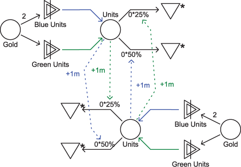
Figure 6.50. Combat with different unit types
We can also add the ability to switch between offensive and defensive modes. This can be modeled using two different pools for attack and defense (Figure 6.51). By moving units from the defense to the attack, you start attacking your enemy. In this case, color coding can be used to prevent immobile units (such as towers or bunkers) from rushing toward the attack.
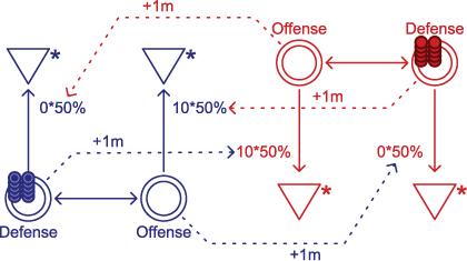
Figure 6.51. Offensive and defensive modes
Technology Trees
Real-time strategy games, but also simulation games like Civilization, often allow the player to spend resources to research technological advances that will give him an extra edge in the game. These constructions are usually referred to as technology trees and often add interesting long-term investments to a game’s economy. More often than not, the technology tree involves multiple steps and many possible routes to various advancements; these technology trees constitute interesting internal economies in their own right.
To model technology trees, you should use resources to represent technological advances and have these resources unlock new game options or improve old ones. Figure 6.52 illustrates how a technology tree can be used to unlock and improve the abilities of a new unit type in a strategy game. The player can start building knights only after he researches one level of knight lore. Every level of knight lore also increases the effectiveness of the knights, although the research gets more and more expensive for every level. In this example, researching knight lore requires a considerable investment but rewards the player with stronger units.
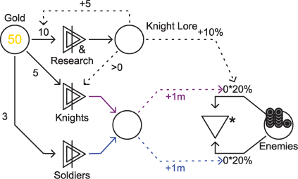
Figure 6.52. Adding research to a strategy game
In some technology trees, players can research each technology only once; however, many technologies require the player to have researched one or more technologies before. For example, Figure 6.53 represents a technology tree that is not unlike the one found in Civilization. Keep in mind that the effect of having a particular technology is omitted from this diagram. However, it is easy to imagine that technologies such as the alphabet and writing increase the resources available for research. In this diagram, the red connections enforce the order in which technologies must be researched, while the blue construction keeps track of the number of resources developed and adjusts the research prices accordingly.
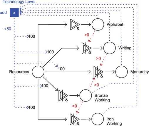
Figure 6.53. A Civilization-style technology tree
Summary
In this chapter, we introduced a few additional features of the Machinations Tool and then took a much closer look at two important mechanics design tools: feedback loops and randomness. We explained seven different characteristics of feedback: type, effect, investment, return, speed, range, and durability. Each of these has a distinct effect on the behavior of an internal economy.
In the section “Randomness vs. Emergence,” we showed how you can use randomness to create unique situations that force players to improvise. We also explained that randomness can help prevent dominant strategies: Because randomness changes a game’s state unpredictably, you are less likely to create a game in which one strategy is always the best one.
We ended the chapter with an extensive discussion of ways to use Machinations diagrams to model economic structures in traditional genres of video games. Machinations can simulate some of the key economies found in action games, role-playing games, first-person shooters, and real-time strategy games.
In the next chapter, we’ll discuss the important topic of design patterns, which are familiar structures that you can use to create and test mechanics quickly.
Exercises
1. Find a way to include an extra negative feedback loop in Monopoly.
2. Create a game in which all random effects affect all players equally.
3. Design the mechanics for a racing game that involves positive, constructive feedback yet remains fair.
4. Create a diagram for the major feedback loops in a published game.
5. Prototype and playtest a game with one feedback loop. Keep adding feedback loops of different signatures until you have an enjoyable, well-balanced game that exhibits emergent behavior. Prototype and play test every step. How many feedback loops are required?
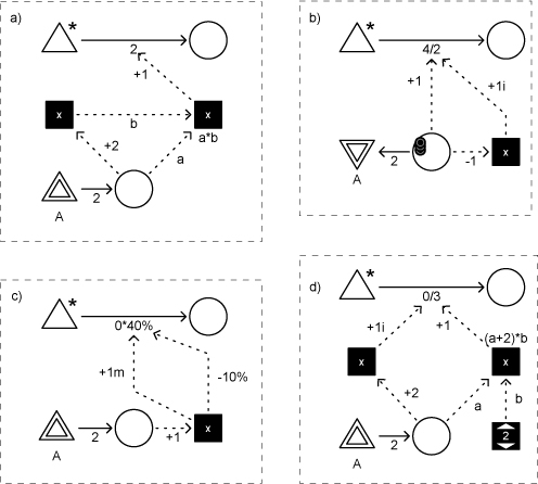
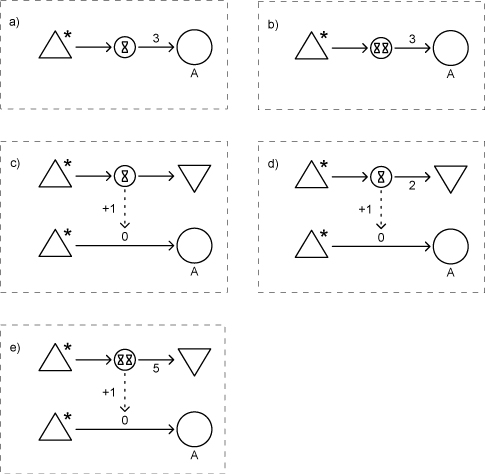
6. In each of the following four diagrams, what will be the production rate of the automatic source at the upper left after clicking the interactive node A exactly once?
7. In each of the following five turn-based diagrams, how many turns will it take to accumulate 10 resources in pool A? (In the Machinations Tool, you would also need an interactive node labeled End Turn to end a turn, but try to figure it out for yourself.)
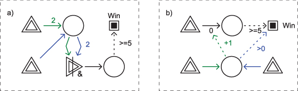
8. In each of these two color-coded diagrams, what is the minimum number of clicks required to win the game?.