Chapter 5. Machinations
In the previous chapter, we showed how a game’s internal economy is one important aspect of its mechanics. We used diagrams to visualize economic structures and their effects. In this chapter, we introduce the Machinations framework, or visual language, to formalize this perspective on game mechanics. Machinations was devised by Joris Dormans to help designers and students of game design create, document, simulate, and test the internal economy of a game. At the core of this framework are Machinations diagrams, a way of representing the internal economy of a game visually. The advantage of Machinations diagrams is that they have a clearly defined syntax. This lets you use Machinations diagrams to record and communicate designs in a clear and consistent way.
We will be using Machinations diagrams throughout this book, so it is important that you learn how to read them. This chapter will take you through most of the elements that make up a Machinations diagram. However, a word of caution: The Machinations framework is a lot to take in at once. The framework comprises many interrelated concepts that are best understood together. This means there is no real natural starting point to explain all these concepts. We have tried to introduce the elements of a Machinations diagram in a logical order, but don’t be surprised if you find yourself referring to earlier concepts on occasion.
Machinations is more than just a visual language for creating diagrams, however. Dormans has built an online tool for drawing the diagrams and simulating them in real time. With it, you can construct and save Machinations diagrams easily, and you can also study the behavior of your internal economy. You can find the tool at www.jorisdormans.nl/machinations.
Appendix C (which you can find online at www.peachpit.com/gamemechanics) includes a tutorial on how to use the Machinations Tool. You can find a quick reference guide to the most important elements of Machinations diagrams in Appendix A.
The Machinations Framework
Game mechanics and their structural features are not immediately visible in most games. Some mechanics might be apparent to the player, but many are hidden within the game code. We need a way to describe and discuss them.
Unfortunately, the models that are sometimes used to represent game mechanics, such as program code, finite state diagrams, or Petri nets, are complex and not really accessible for designers. Moreover, they are ill-suited to represent games at a sufficient level of abstraction, in which structural features such as feedback loops are immediately apparent. Machinations diagrams are designed to represent game mechanics in a way that is accessible yet retains the structural features and dynamic behavior of the games they represent.
The theoretical vision that drives the Machinations framework is that gameplay is ultimately determined by the flow of tangible, intangible, and abstract resources through the game system. Machinations diagrams represent these flows, and they let you see and study the feedback structures that might exist within the game system. These feedback structures determine much of the dynamic behavior of game economies. By using Machinations diagrams, a designer can observe game systems that would normally be invisible. Figure 5.1 provides an overview of the Machinations framework and its most important components.
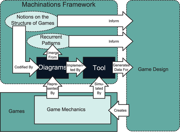
Figure 5.1. The Machinations framework
The Machinations Tool
You can draw Machinations diagrams on paper or with a computerized drawing tool. At the same time, the syntax of the language is exact. It describes unambiguously how different elements of an internal economy interact. The syntax of the Machinations language is formal enough to be interpreted and executed on a computer; it is close to a visual programming language designed to represent game mechanics.
Digital Machinations diagrams are dynamic and interactive representations of game mechanics. Unfortunately, we can’t show their dynamic and interactive nature in the static illustrations printed in this book. However, Dormans has created a free, online application named the Machinations Tool. The tool lets you draw Machinations diagrams, simulate their operation in real time, and interact with them. On the Machinations website, you can find interactive versions of many of the examples that we discuss in this and later chapters. To a certain extent, the digital versions of Machinations diagrams are playable. Some diagrams are so much like playing an actual game that experimenting with them is fun and challenging in itself.
You can find the Machinations Tool, and many resources for using it, at www.jorisdormans.nl/machinations.
How the Machinations Tool Works
A static Machinations diagram, such as the ones printed in this book, can display only one distribution of resources. However, the Machinations Tool allows you to load digital versions of the diagrams and see how they change over time.
The Machinations Tool looks similar to an object-oriented 2D drawing application such as Microsoft Visio. It has a workspace in the middle and a variety of selectable tools in a side panel. You can create diagrams in the workspace or load them from a file.
When you tell the tool to run, it performs the events that are specified by the diagram in a series of time steps or iterations (we use the terms interchangeably). The tool changes the state of the diagram. When it has completed one iteration, the tool then executes another with the diagram in its new state, and so on, repeatedly until you tell it to stop. (You can also build a feature into the diagram that will cause iteration to stop automatically when certain conditions are met—like when the clock runs out in basketball.) You can control the length of each time step by setting an interval value; if you want the tool to run slowly, you can set the interval to several seconds per time step.
Scope and Level of Detail
In earlier chapters, we discussed the notion of abstraction: the process of simplifying or eliminating details of a system to make it less complex and easier to study and tune. For example, the computers that ran the early versions of SimCity did not have enough CPU power to represent each automobile individually. Instead, the game simply computed traffic density in a general way along each stretch of road and displayed an animation that showed how dense it was.
Machinations diagrams permit you to abstract as much or as little as you like. You can use them to focus on all, or only part, of a game’s mechanics. Using Machinations diagrams, you can design and test your game’s mechanics at different levels of detail. How you use them depends on what you want to achieve. For example, it’s often sufficient to model a game from the perspective of a single player, even if the game is actually played by multiple players. Once you’ve done that, it’s fairly easy to imagine how a diagram might be duplicated and the duplicates combined to represent the multiplayer situation.
In other cases, it’s useful to model the mechanics for one player at a higher level of detail than other players. Or you can leave out certain aspects of the game, such as players taking turns. At a high level of abstraction, there is often little difference in the effects of real-time play and turn-based play.
For the examples in this book, we have tried to keep the level of detail low and the level of abstraction high so the diagrams don’t get too complex. This way, you can easily see the structural features of the internal economy, which will help you to understand how these structures create emergent gameplay. For this reason, the natural scope of a Machinations diagram is that of a single player and that player’s individual perspective on the game system. Although it is certainly possible to model multiplayer systems and turn-based play, the framework, as it currently stands, does not include features designed to support multiplayer games in particular. For example, the main input device for interaction with a Machinations diagram is the mouse; there is no support for multiple players using multiple input devices. The tool has no means of enforcing whose turn it is to interact or to prevent one player from clicking a part of the diagram that belongs to another player. It’s a simulation tool, not a tool for building playable games.
Finally, a word of caution: We have used Machinations diagrams to model a number of real games, but as we said, we have intentionally simplified them in this book. The Machinations framework and diagrams only facilitate understanding of games; they aren’t a substitute for studying the game itself.
Machinations Diagram Basic Elements
The Machinations framework is designed to model activity, interaction, and communication between the parts of a game’s internal economy. As shown in the previous chapter, a game’s economic system is dominated by the flow of resources. To model a game’s internal economy, Machinations diagrams use several types of nodes that pull, push, gather, and distribute resources. Resource connections determine how resources move between elements, and state connections determine how the current distribution of resources modifies other elements in the diagram. Together, these elements form the essential core of Machinations diagrams. Let’s take a look at these basic elements.
Pools and Resources
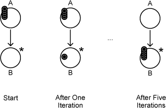
The most basic node type in a Machinations diagram is the pool. A pool is a location in the diagram where resources gather. Pools are represented as open circles, while the resources that are stored in a pool are represented as smaller, colored circles that stack on them (Figure 5.2). If there are too many resources in a pool to show them as stacks, the tool displays a number instead.

Figure 5.2. Pools and resources
You can change the threshold at which the tool switches from displaying stacks to displaying numbers in a pool. With the pool highlighted, enter a value in the Display Limit box at the side panel. The default is 25. If you enter a value of zero, the pool will always display a number, unless it is empty. You can set a different value for each pool you create.
Pools are used to model entities. For example, if you have a resource called money and an entity called the player’s bank account, you would use a pool to model the bank account. Note, however, that pools cannot store fractional values, only integers. The bank account would have to contain only whole dollars or to be characterized in terms of cents rather than dollars.
Machinations uses different colors to distinguish among different types of resources. A pool can contain resources of more than one type, which means that it can be used to model compound entities. However, until you are familiar with the Machinations framework, it is best not to mix different resources in a single pool. It is easier to have separate pools to, for instance, represent the health, energy, and ammunition of a single player, than it is to have one pool with different colored resources to represent all of them.
Resource Connections
Individual resources can move from node to node through a Machinations diagram along resource connections that are represented as solid arrows connecting the nodes of the diagram (Figure 5.3).
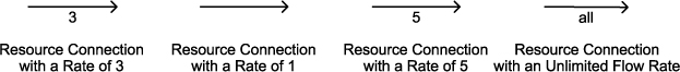
Figure 5.3. Resource connections
Resource connections can transfer resources at different rates. A label beside the resource connection indicates how many resources can move along the connection in a single time step. If a resource connection has no label, its rate is considered to be 1. You can also make a resource connection transfer an unlimited number of resources in a single time step by using the word all as the resource connection’s label.
To help you see how an internal economy works, the Machinations Tool shows the resource flow by animating the movement of the resources along the resource connections. When the tool runs, you will see the resources traveling along the connection lines from one node to another.
Remember that a pool is one type of node. There are seven other types of nodes, each of which serves a specialized purpose. They are described in the section “Advanced Node Types.”
To enter a fixed flow rate for a resource connection in the Machinations Tool, select the resource connection and then type a number or the word all in the Label box in the side panel.
If you do not want to watch the resources move along the resource connections, you can run the Machinations Tool in Quick Run mode. You will find this under the Run tab in the side panel. This will make the tool run much faster.
As we have explained, games frequently use random number generators to create uncertainty. To model these kinds of games accurately, you can specify random flow rates in Machinations diagrams by entering them in the Label box. Random rates are represented in different ways. If you simply enter D, a die symbol (![]() ) will appear beside the resource connection to indicate an unspecified random factor. It means that the rate varies somewhat, but you don’t want to specify the details precisely. (If you actually simulate the diagram in the Machinations Tool, it will use the default value given in the Dice box in the side panel.)
) will appear beside the resource connection to indicate an unspecified random factor. It means that the rate varies somewhat, but you don’t want to specify the details precisely. (If you actually simulate the diagram in the Machinations Tool, it will use the default value given in the Dice box in the side panel.)
Figure 5.5. Different notations for random flow rates
Activation Modes
In each iteration, the nodes in a Machinations diagram may fire. When a node fires, it pushes or pulls resources along the connections that are connected to it (we explain this in the next section). Whether a node fires depends on its activation mode. A node in a Machinations diagram can be in one of four different activation modes:
• A node can fire automatically, which means it simply fires every iteration. All automatic nodes fire simultaneously.
• A node can be interactive, which means it represents a player action and fires in response to that action. In a digital version of a Machinations diagram, interactive nodes fire after the user clicks them.
• A node can be a starting action, which means that it fires only once, before the first iteration. In the Machinations Tool, starting actions fire immediately after the user clicks the run button.
• A node can be passive, which means it can fire only in response to a trigger generated by another element (we discuss triggers shortly).
Each type of node looks different so you can tell them apart (Figure 5.6). Automatic nodes are marked with an asterisk (*), interactive nodes have a double outline, starting actions are marked with an s, and a passive node has no special mark.
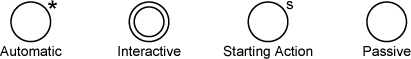
Figure 5.6. Activation modes
Pulling and Pushing Resources
When a pool fires, it will try to pull resources through any inputs connected to it. The number of resources it pulls is determined by the rate of the individual input resource connection—the number beside the line. Alternatively, a pool can be set in push mode. In this mode, when the pool fires, it pushes resources along its output connections. Again, the number of resources pushed is determined by the flow rate of the output resource connection. A pool in push mode is marked with a p (Figure 5.7). A pool that has only outputs is always considered to be in push mode, in which case the p marker is omitted.
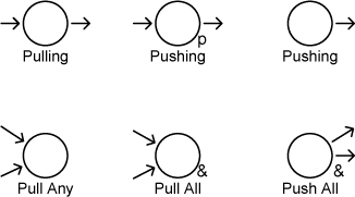
Figure 5.7. Pull and push modes
If a pool is trying to pull more resources than exist at the far end of its inputs, it will handle it in one of two ways:
• By default, a node pulls as many resources as it can, up to the flow rates of its inputs. If not enough resources are available, it still pulls those that are.
• Alternatively, a node can be set to pull all or no resources. In this mode, when not all resources are available, none are pulled. Nodes that are in all or none pull mode are marked with an & sign (Figure 5.7).
These rules also apply to pushing nodes: By default, a pushing node sends as many resources as are available out along its output resource connection up to the output’s flow rate. A pushing node in all or none mode sends resources only when it can supply all of its outputs. This means that nodes in push mode might be marked with both a p and an &.
Figure 5.8 illustrates two situations in which there are not enough resources to meet the demand. Node A is user-activated (which is why you see the double line). It wants to pull three resources from its upper input and two from its lower one, but the pools they are connected to do not contain enough resources to do it. When clicked, node A will simply pull the resources that are available.

Figure 5.8. Two examples showing fewer resources than requested
When node B is clicked, it tries to pull a random number, from one to six, of resources from its input. If the random number is four, five, or six, it will pull the three that are available.
Time Modes
Games can handle time in different ways. Board games are often turn-based, while in many video games the game is active even if the player doesn’t do anything. To represent different types of games, a Machinations diagram can operate in one of three different time modes:
• In synchronous time mode, all automatic nodes fire at a regular interval that you can specify for the whole system. All interactive nodes that you click fire at the next time step, at the same time when automatic nodes fire. In this mode, all actions in one time step take place simultaneously. It is possible for a user to activate several different interactive nodes during a time step, but each interactive node can be activated only once in a time step.
You can set the time mode of a diagram in the Machinations Tool by using the Time Mode pull-down menu visible in the side panel when no element of the diagram is selected. In either synchronous or asynchronous mode, you can set the length of the interval in the Interval box, in units of a second. The Interval box also accepts fractional values, so 2.5 means each time step lasts 2.5 seconds.
• In asynchronous time mode, automatic nodes in the diagram are still activated at regular intervals of arbitrary length specified by the user. However, players can activate interactive nodes at any time within the intervals, and the resulting actions are executed immediately, without waiting for the next time step. In this case, an interactive node can be activated multiple times during a time step. This is the default setting of the Machinations Tool.
• Alternatively, a Machinations diagram can be in turn-based mode. In this mode, time steps do not occur at regular intervals. Instead, a new time step occurs after the player has executed a specified number of actions. This is implemented by assigning a number of action points to each interactive node and allotting players a fixed budget of action points each turn. After all the action points are used, all the automatic nodes fire, and a new turn starts.
If you set the time mode to turn-based in the Machinations Tool, the Interval box is replaced by an Actions/Turn box, in which you can specify the number of action points permitted in a single turn. To specify the number of action points that an interactive node consumes when clicked, select the node and enter a value in the Actions box in the side panel. You may also enter a value of zero. When all interactive nodes cost no action points, except a single interactive node named “end turn” (that has no other effect), this can be used to create a game where players can take any number of actions until they indicate that they are finished.
Figure 5.10. How simultaneous pulls are handled in a Machinations diagram depends on the diagram’s time mode.
State Changes
The state of a Machinations diagram refers to the current distribution of resources among its nodes. When the resources move from one place to another, the state changes. In the Machinations framework, you can use state changes to modify the flow rates of resource connections. In addition, you can trigger nodes to fire, or activate or deactivate them, in response to changes in resource distribution.
It can be confusing to run the Machinations Tool and watch a label modifier causing its target to decrease even though the label modifier’s own label is positive. Think of it this way: A positive label on the label modifier causes its target to follow the origin node, going up when the origin goes up and going down when it goes down. A negative label on the label modifier causes its target to invert the origin node, going down when the origin goes up, and vice versa.
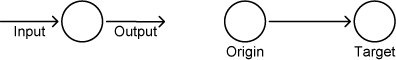
To make this possible, Machinations offers a second class of connections called state connections. State connections indicate how changes to the current state of a node (the number of resources in it) affect something else in the diagram. State connections are shown as dotted arrows, leading from the controlling node (called the origin) and going to a target, which can be either a node, a resource connection, or, rarely, another state connection. Labels on the state connection indicate how it changes the target. There are four types of state connections that are characterized by the type of elements they connect and their labels. The four types are label modifiers, node modifiers, triggers, and activators. We explain them in each of the following four sections.
Label Modifiers
Remember that a label on a resource connection determines how many resources may move through that connection in a given time step. Label modifiers connect an origin node to a target label (L) of a resource connection (or even another state connection). A label modifier indicates how state changes in the origin node (ΔS) modify the current value of the target label at a current time step (Lt) as indicated by the state connection’s own label (M). The new value takes effect in the next time step (Lt+1). The amount of the change in the origin node is multiplied by the label multiplier’s own label. So, if the label modifier says +3 and the origin node increases by 2, then the target label will increase by 6 in the next time step (it will add 3 twice, once for each change in the origin node). However, if the label modifier says +3 and the origin node decreases by 2, then the target label will decrease by 6. Thus, the new value of label (Lt+1) that is the target of a single label modifier is given by the following formula:
Lt+1 = Lt + M × ΔS
If the label is the target of multiple label modifiers, you will have to take the sum of all the changes to find the new value:
Lt+1 = Lt + ∑ (M × ΔS)
This is the first time we have used color in a Machinations diagram. Here, it is used only for visual clarity. However, the diagrams can also be color-coded, a special feature of the Machinations Tool. We explain colorcoding in more detail in Chapter 6.
The label of a label modifier always starts with a plus or minus symbol. For example, in Figure 5.11, every resource added to pool A adds 2 to the value of the resource flow between pools B and C. Thus, the first time B is activated, one resource flows to A and three resources flow to C. The second time, one resource still flows to A, but now five resources flow to C.
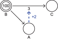
Figure 5.11. A label modifier affecting the flow rate between two pools. At a given time step, the flow from B to C is 3 + 2 times the number of items in A.
Figure 5.12 is not meant to be simulated in the Machinations Tool; it only illustrates the principle.
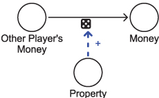
Figure 5.12. In Monopoly the state of your property positively affects the chance other players’ money flows to you.
Label modifiers are frequently used to model different aspects of game behavior. For example, a pool might be used to represent a player’s accumulated property in a game of Monopoly. The more property a player has, the more likely it is that player will collect money from other players. This can be represented by the diagram in Figure 5.12. Note that in this case the exact value of the label modifier is unspecified; it indicates only that the effect on the random flow rate is positive. Also note that many mechanics of Monopoly are omitted in this diagram—for example, the diagram does not show how a player acquires property. You will find diagrams that paint a more complete picture of Monopoly in Chapters 6 and 8.
Node Modifiers
Node modifiers connect two nodes. They enable changes in the state of one node (its origin) to modify the number of resources in another node (the target node), according to the node modifier’s label (M). When the origin node changes, it influences the target node in the next time step. More than one origin node can modify a target node. The formula for this is nearly identical to the formula used for label modifiers:
Nt+1 = Nt + ∑ (M × ΔS)
Notice that node modifiers can create and destroy resources if their target is a pool. This is all right for an abstract resource such as “threat level” but is best avoided for tangible and intangible resources such as “keys” or “health.” To create and destroy those kinds of resources, use other types of nodes called sources and drains, described later in this chapter.
Figure 5.13 illustrates a node with two modifiers. The number of resources in C will be equal to three times the number in A, minus two times the number in B.
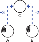
Figure 5.13. Node modifiers affect the number of resources in a pool.
Node modifiers can have labels that are fractions, for example +1/3 or -2/4. In this case, the number of resources of a target node is modified by the value indicated by the fraction’s numerator every time there is a change to the number of resources on the origin divided by the fraction’s denominator and rounded down. Thus, when the number of resources on an origin node changes from 7 to 8, the number of resources on the target is lowered by 2 if the modifier is -2/4, but if the modifier is +1/3, the number of resources on the target node does not change.
This sounds complex, but a simple example of the use of node modifiers can be found in a real game. In The Settlers of Catan, players gain one point for every village in their possession and two points for every city in their possession. The number of villages is one origin node, the number of cities is a second origin node, and both modify the target node, which is the player’s number of points.
Triggers
Triggers are state connections that connect two nodes or connect an origin node to the label of a resource connection. Triggers are identified by their label, which is an asterisk (*). Triggers do not change numeric values the way label and node modifiers do. Rather, a trigger fires when all the inputs of its origin node become satisfied: when each input brings in the number of resources to the node as indicated by its flow rate. A firing trigger will in turn fire its target. When the target is a resource connection, the resource connection will pull resources as indicated by its flow rate. A node that has no inputs will fire outgoing triggers whenever it fires (either automatically or in response to a player action or to another trigger).
Triggers are commonly used to fire passive nodes that do nothing until the trigger fires them. This enables you to set up a passive node that fires only when certain circumstances arise in the game.
Triggers are commonly used in games to react to the redistribution of resources. For example, in Monopoly players might transfer money to the bank in order to trigger the transfer of property from the bank into their possession. This can be represented as the diagram in Figure 5.14.
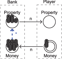
Figure 5.14. A trigger in Monopoly enables the acquisition of property by spending money.
Activators
Activators connect two nodes. They activate or inhibit their target node based on the state of their origin node and a specific condition. The activator’s label specifies this condition. Conditions are written as an arithmetic expression (for example, ==0, <3, >=4, or !=2) or a range of values (for example, 3-6). If the state of the origin node meets this condition, then the target node is activated (it can fire). When the condition is not met, the target node is inhibited (it cannot fire).
Activators are used to model many different game mechanics. For example, in the board game Caylus, players place their laborers (a resource) at particular buildings on the board to enable them to execute special actions associated with that building. For example, a player might place a laborer at a gold mine to collect gold (Figure 5.15). However, as indicated by the trigger in the figure, in Caylus every time a player mines gold, the laborer then returns to the player’s Workers pool.
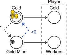
Figure 5.15. Caylus
Advanced Node Types
Pools are not the only possible nodes in a Machinations diagram. In this section, we will describe seven more types of nodes that you can use, including special nodes for the four economic functions (sources, drains, converters, and traders) discussed in the previous chapter. However, as you will see, some of these nodes can actually be re-created by using clever constructions of pools, resource connections, and state connections. Dormans has created these specialized node types to make the diagrams easier to read. If Machinations diagrams were restricted only to pools, the diagrams would quickly become cluttered.
Gates
In contrast to a pool, a gate does not collect resources. Instead, it immediately redistributes them. Gates are represented as diamond shapes that often have multiple outputs (Figure 5.16). Instead of a flow rate, each output is labeled with a probability or a condition. The first type of outputs are referred to as probable outputs while the others are referred to as conditional outputs. All outputs of a single gate must be of the same type: When one output is probable, all must be probable, and when one output is conditional, all must be conditional.
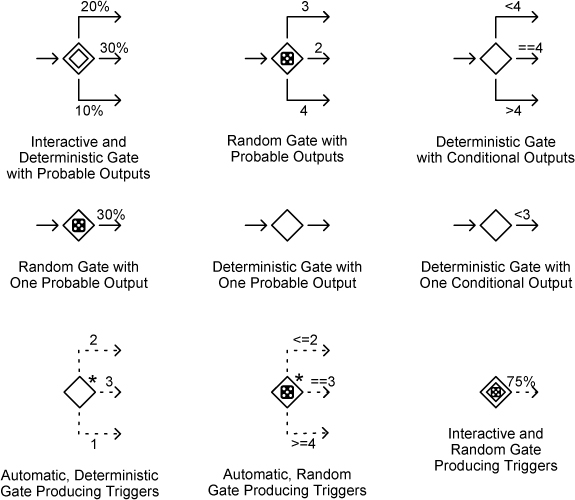
Figure 5.16. Different types of gates in a Machinations diagram
Probabilities can be represented as percentages (for example, 20%) or weights indicated by single numbers (for example, 1 or 3). In the first case, a resource flowing into a gate will have a probability equal to the percentage indicated by each output. The sum of these probabilities should not add up to more than 100%. If the total is less than 100%, there is a chance that the resource will not be sent along any output and be destroyed instead. In the case of weights, the chance that a resource will flow through a particular output is equal to the weight of that output divided by the sum of the weights of all outputs of the gate. In other words, if there are two outputs, one with a weight of 1 and the other with a weight of 3, the chance that a resource will flow out the first one is 1 in 4, and the chance that it will flow out the second one is 3 in 4.
Gates with probable outputs can be used to represent chances and risks. For example, in Risk players put armies in danger to gain territories. This type of risk can be represented easily by a gate with probable outputs indicating the rates for success or failure.
An output is conditional when it is labeled with a condition (such as >3 or ==0 or 3-5). In this case, all conditions are checked every time a resource arrives at the gate, and one resource is sent along every output whose condition is met. The conditions might overlap; this can lead to duplication of resources or, when no condition is met, to the destruction of the resource.
Like pools, gates have four activation modes: Gates can be passive, interactive, or automatic, or they can be a starting action. Interactive gates have a double outline, automatic gates are marked with a star, and gates that are activated once before the diagram starts are marked with an s. When a gate has no inputs, it triggers every time it fires. This way gates can be used to produce triggers either automatically or in response to player actions.
Gates have one of two distribution modes: deterministic distribution and random distribution. A deterministic gate will distribute resources evenly according to the distribution probabilities indicated by percentages or weights if it has probable outputs. When it has conditional outputs, it will count the number of resources that have passed through it every time step and will use that number to check the conditions of its outputs. (It can be convenient to think of a deterministic gate with conditional outputs as a counting gate.) A deterministic gate has no special symbol and is represented as a small open diamond.
When you place a gate in a Machinations diagram in the tool, you may set the gate’s type by clicking one of the Type icons in the side panel. The hollow diamond (the default) is a deterministic gate. The die symbol converts it to a random gate.
A random gate generates a random value to determine where it will distribute incoming resources. When it has probable outputs, it will generate a suitable number (either a value between 0% and 100% or a number below the total weights of the outputs). When its outputs are conditional, it will produce a value between 1 and 6 to check against the conditions, just as if the diagram rolled a normal six-sided die (later we will show you how this value can be changed to represent other types of random distribution). Random gates are marked with a die symbol.
Gates might have only one output. Gates with one output act the same way as gates with multiple outputs. The gates on the middle row of Figure 5.16 will (from left to right) randomly let 30% of all the resources pass, immediately pass the resource to the output regardless of the output’s flow rate, and let only the first two resources pass.
All output state connections from a gate are triggers; gates do not accumulate resources, and therefore label modifiers, node modifiers, and activators originating from a gate serve no purpose. These triggers can also be conditional or probabilistic. In this way, gates can be used to control the flow of resources (Figure 5.17).
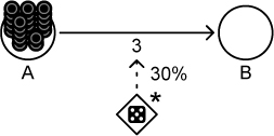
Figure 5.17. An automatic, random gate controlling the flow of resources between two passive pools. In this case, there is a 30% chance that three resources will flow from A to B every time step.
Sources
Sources are nodes that create resources. They are represented as a triangle pointing upward (Figure 5.18). Any node in a Machinations diagram can be automatic (the default), interactive, or passive, or it can activate once before a diagram starts. An example of an automatic source is the steady regeneration of the protective shields of the player’s star fighter in Star Wars: X-Wing Alliance. The action to build armies in Risk would be modeled as an interactive source of armies, and passing Go in Monopoly would be a passive source of money that is triggered by a game event. The rate at which a source produces resources is a fundamental property of a source and is indicated by the flow rates of its outputs.
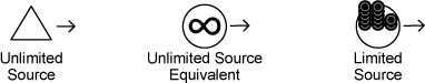
Figure 5.18. Unlimited and limited sources
In many ways, a source acts just as a pool without inputs that starts with a sufficiently large (or even infinite) supply of resources. However, to model limited sources (see the section “Four Economic Functions” in Chapter 4), it is better to use a pool with a specified number of resources in it.
Drains
Drains are nodes that consume resources; a resource that goes into a drain disappears permanently. The Machinations framework includes a special drain node represented as a triangle pointing downward (Figure 5.19). The rate of a drain is determined by the flow rate of its input resource connection. Some drains consume resources at a steady rate, while others consume resources at random rates or intervals. You can also make a drain consume everything its input resource connection is attached to by labeling the resource connection with all. (A toilet is a good example: When flushed, it drains all the water in the cistern, no matter how much it is.) You could in principle represent a drain as a pool with no outputs, but to indicate that the resources that flow to a drain are consumed and have no further impact on the game, it is better to use a drain node.
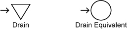
Figure 5.19. Drains
Drains are useful for representing processes that remove resources from an economy permanently. This might include the effect of wear or friction in a physical system or the consumption of ammunition when a weapon is fired in a shooter game.
Converters
Converters convert one resource into another. They are represented as a triangle pointing to the right with a vertical line through it (Figure 5.20). Converters are designed to model things like factories that turn raw materials into finished products. A windmill, for example, turns wheat into flour. Converters act exactly as a drain that triggers a source, consuming one resource to produce another. As with sources and drains, converters can have different types of rates to consume and produce resources as specified by their inputs and outputs. For example, a converter representing a sawmill might turn one tree into 50 boards of lumber.
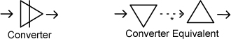
Figure 5.20. Converters
Since converters are constructed from drains and sources, it is possible to create a special construction that might be called a limited converter that can produce only a limited amount of something as its output. A limited converter is the combination of a drain and a limited source. Figure 5.21 shows two equivalent alternatives to construct a limited converter.
Figure 5.21. Two ways to build a limited converter
Traders
Traders are nodes that cause resources to change ownership when fired: Two players could use a trader to exchange resources. Machinations diagrams represent a trader as a vertical line over two triangles that point left and right (Figure 5.22). Use traders when a given number of resources of one type is exchanged for (not converted into) a given number of another type. This is ideal for any situation that resembles shopping: the merchant receives money, and the customer receives goods in a stated proportion (the price). If either the merchant or the customer does not have the necessary resources, the trade cannot take place. Fallout 3, in which all traders’ supplies are limited, is a good example. A trading mechanism can be constructed by two gates connected by a trigger ensuring that when one resource is received, the other is returned in exchange.
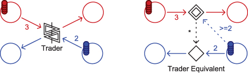
Figure 5.22. Traders
This is an example of a color-coded diagram, which uses color to represent different kinds of resources. In Figure 5.22, think of red as representing money and blue as representing goods. When the interactive Trader icon is clicked, three money resources are exchanged for two goods resources. We explain color-coded diagrams in more detail in Chapter 6.
End Conditions
Games end when certain conditions are fulfilled. Sometimes they end when a player reaches a certain goal or when time runs out or when all players but one are eliminated. Machinations diagrams use end conditions to specify end states. The Machinations Tool checks the end conditions in a diagram at each time step and stops running immediately when any end condition is fulfilled. End conditions are square nodes with a smaller, filled square inside (the same symbol that is used to indicate the stop button on most audio and video players). End conditions must be activated by an activator. The activators are used to specify the end state of the game. Figure 5.23 shows a couple of examples. The diagram on the left stops after the 25 resources are drained automatically. In the example on the right, you win by growing more than three apples and oranges.
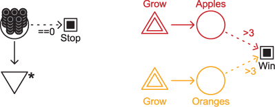
Figure 5.23. End conditions
Modeling Pac-Man
Let’s see how you can use Machinations diagrams to simulate the mechanics of a simple game—the arcade classic Pac-Man. We’ll break down the process of modeling Pac-Man into six steps and add them to a Machinations diagram, one at a time to show how they work. First we’ll identify the game’s most important resources, and then we’ll model the individual mechanisms. We’ll give each major mechanism its own color for ease of identification. The last of these mechanisms ties everything together into a full diagram for Pac-Man.
We have to warn you that our model is an approximation, not a literal simulation of what Pac-Man’s software does. For example, we implemented a system in which the ghosts come out of the ghost house at a regular rate, one every five time steps. The real game uses a more complex algorithm to determine when they come out. We could have modeled it, but it would have made the diagram too complex. Our goal here is to teach you to use the Machinations framework, not to create an exact copy of the real game, so we have simplified it a bit.
Resources
We will use the following resources to model Pac-Man:
• Dots. Scattered along the maze are the dots that Pac-Man must eat to complete a level. Dots are tangible resources in Pac-Man that must all be destroyed to win. The game starts with a fixed number of dots. Dots are not produced during play (except when going to the next level).
• Power Pills. Every level starts with four power pills, which Pac-Man can eat to be able to eat the ghosts. These power pills are a scarce but tangible resource the player must use wisely. Like dots, they are only consumed, never produced during play.
• Fruits. Occasionally a fruit appears in the maze. Pac-Man can eat the fruit to score extra points.
• Ghosts. There are four ghosts that chase Pac-Man around the maze. The ghosts can be in one of two locations: Either they are in the “ghost house” (the area in the middle of the screen) or they are in the maze giving chase. The ghosts are also a tangible resource. (Notice that resources are not always positive things for the player!)
• Lives. Pac-Man starts the game with three lives. Lives are intangible resources in Pac-Man. If Pac-Man loses all lives, the game ends.
• Threat. To simulate the effect of the ghosts giving chase, we will model an abstract resource called threat. When the threat passes a certain threshold, Pac-Man is caught, and he loses a life. Note that we are not modeling the shape of the maze itself (which Machinations cannot do), only the flow of resources and states the game can be in.
• Points. Every time Pac-Man eats a dot, a fruit, or a ghost, he will consume them and score a number of points. The objective of the game is to score as many points as possible. Points are intangible resources.
These are all the obvious resources in the Pac-Man economy, and we’ll start our model by constructing systems around them. Notice that threat is one we made up for the purposes of the simulation, and our decisions about how to model threat are subjective and not part of the original game.
Dots
We start with a simple mechanic: Pac-Man eats dots, converting them into points. It can be represented with two pools and a converter (Figure 5.24). One pool starts with 50 resources in it representing the dots in the maze. The pool that collects points starts empty. We also added an end condition that determines that you have completed a level after eating all the dots. The converter representing the eating action is an interactive node. You can click it to eat the dots. Notice, however, that the input of the converter has a random flow rate. Every time you click, there is only a partial chance that the action succeeds. The more dots there are, the easier it is to eat them. Initially the chance to eat a dot starts at 100%, but every iteration, for every dot that is eaten, the chance is lowered by 1%. This reflects the challenge to the player in moving around the maze and eating every single dot.
The real game has exactly 240 dots on every level. We reduced this to 50 to make the game shorter.
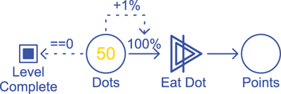
Figure 5.24. Eating dots to score points
Don’t be confused by the fact that the probability of successfully eating a dot goes down even though the state connection that controls it is labeled +1%. Remember that the function of the state connection is to transmit the change in its origin pool (multiplied by its label). Because in this case the change is always negative, the state connection actually transmits a negative value.
In the real game, Pac-Man eats dots 100% of the time until he returns to a place he has already been, at which point he eats dots 0% of the time. We had to approximate this somehow, so we used a diminishing probability of successfully eating a dot every time the Eat Dot converter is clicked. In our model, the probability of eating a dot is initially set to 100%, modified by a label modifier that reflects changes in the Dots pool. If the number of dots in the Dots pool changes between one time step and the next, that change is multiplied by the label on the state connection, and the result is applied to the percentage on the resource connection. When a dot is consumed (say, from 50 dots to 49), the change in the state of the Dots pool is -1. Multiply that by +1% and you get -1%, and that reduces the probability of successfully eating a dot by 1% on the next time step.
The process of creating these approximations is one of the trickier aspects of modeling a game with Machinations, and you have to think carefully about what your decisions mean. We chose numbers that feel good to us, but we could have used others. For example, we could have chosen a rate of change of 0.25% instead of 1% for successfully eating a dot. This would represent a very skilled player who spends little time in parts of the maze where he has already been—he’s eating new dots most of the time.
In some respects, it’s easier to model a new game than an existing one. When you use Machinations to design a new game, you can set up anything you want. The tool’s greatest strength is that you can experiment and adjust the details as much as you like.
The Fruit Mechanism
The fruit mechanism (Figure 5.25) works similarly to the dot mechanism. However, in contrast to dots, a fruit will appear from time to time and disappear automatically if Pac-Man doesn’t eat it. These extra mechanics are represented by the source and the drain that are connected to the fruit pool. The fractional rates indicate that the fruit source produces a fruit once every 20 iterations and is drained once every 5 iterations. This means a fruit will appear once every 20 iterations and disappear 5 iterations later. The interactive node that represents the Eat Fruit action has a fixed chance of 50% to actually succeed. This approximates the difficulty of catching the fruit as it moves through the maze. However, eating a fruit will produce 5 points instead of 1 as eating a dot does.
In the real game, fruit appears only twice in a level and offers an escalating number of bonus points depending on which level it is. We don’t implement multiple levels of the game, so we made the fruit process shorter, simpler, and more frequent so that it is easier to observe.
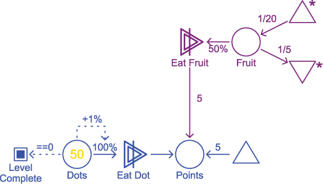
Figure 5.25. Fruit mechanism (purple) added to the diagram
Ghosts Produce Threat
The four ghosts start in the ghost house, and they enter the maze at a fixed rate of one ghost every five iterations. Each ghost that is in the maze will produce a threat, which we represent as a black resource generated by an automatic source. Figure 5.26 represents these mechanics. In this diagram, the Maze pool pulls one ghost every five iterations. Each ghost in the maze increases the output of the source that produces the threat. The player has a chance to lower the threat by clicking the random interactive Evade gate. When clicked, it has a 50% percent chance of triggering a drain that drains nine threat resources. (If this fails, the Evade gate does nothing, but the player may click it again to try again.) We arbitrarily chose this value to indicate that trying to evade the ghosts doesn’t always work. If you wanted to change the diagram to represent a more skilled player, you could increase this percentage.
In the real game, the algorithm that determines when ghosts leave their house is quite complex. We made it simpler for teaching purposes. Also, the ghosts have limited artificial intelligence that governs how they move; that doesn’t appear in our diagram because we don’t simulate the layout of the maze.
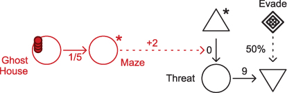
Figure 5.26. Ghosts create threat but can be evaded.
Capture and Loss of Life
When the number of threat resources in the Threat pool passes 100, Pac-Man is caught, and the player loses a life (Figure 5.27). In the meantime, the ghosts return to the ghost house, and the player can start again, unless it was his last life in which case the game is over. This process is represented by an automatic trigger (the black dotted line) that is activated when the number of threat resources passes the threshold of 100. It goes to a Reset gate, which passes the trigger on in three directions (the green dotted lines): to a drain that drains a life, to a resource connection that returns the ghosts from the maze to their house, and to a drain that drains all the built-up threat.
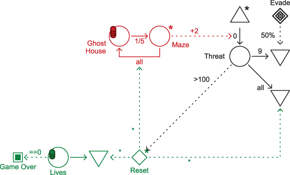
Figure 5.27. Reset when caught
Note the label reading >100 on the state connection to the Reset gate. This indicates that the state connection is an activator. Activators connect two nodes. The first node activates the second node when the condition is met, which, in this case, is when the Threat pool contains more than 100 threat resources.
Power Pills
The last mechanism to be added to the diagram is the mechanism that allows players to eat the ghosts by eating power pills. Figure 5.28 adds this mechanism (light blue) to the diagram and represents the full game. Power pills start as a limited supply. The player can choose to use them by clicking the Eat Power Pill converter to convert a power pill into power-up time, an abstract resource that is automatically drained. While some power-up time remains, the ghosts stop producing threat, and a drain on the threat is activated. At the same time, a new action to eat a ghost becomes available. Eating ghosts returns a ghost to the ghost house and also produces five bonus points.
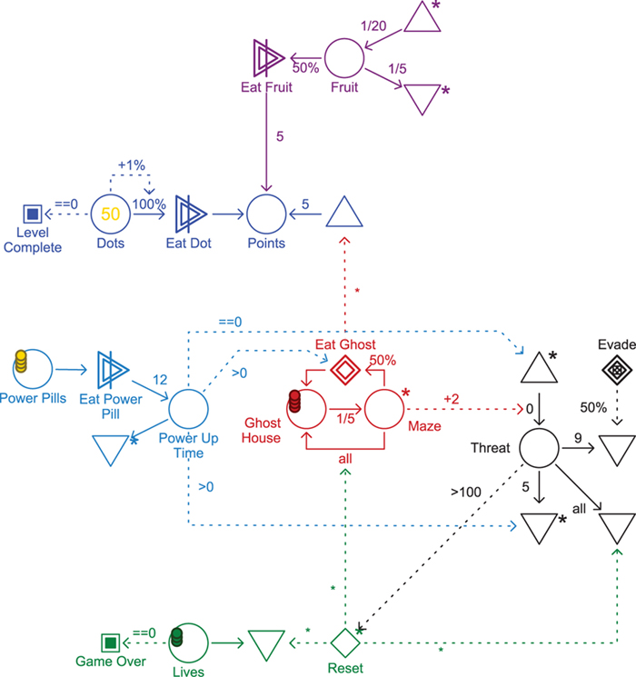
Figure 5.28. Complete diagram for Pac-Man
Because we don’t simulate the layout of the maze, we arbitrarily assigned a value of 100 to the threat level to determine when the player is caught by a ghost. But as in the real game, the player can evade (using the interactive Evade gate), which lowers the threat.
The Complete Diagram
Figure 5.28 represents a playable approximation of Pac-Man. As we have said, certain mechanisms have been omitted, and the game is different in various details. It is possible to add these details to a Machinations diagram, but you would be unlikely to learn anything new from them. However, you can discover a few important things from studying even this simplified diagram. For one thing, players of Pac-Man must balance their activities among different tasks: eating dots, evading ghosts, and eating fruit. One of these actions, eating fruit, is fairly isolated from the rest of the game. Eating fruit scores bonus points but doesn’t help with anything else, which means that novice players who have their hands full with the tasks of eating and evading can safely ignore the fruit. The power pills are an important resource that must be spent wisely.
Playing around with the digital version of the Pac-Man diagram even gives you a feel of some of the strategic options available in the real game: You can use power pills to eat ghosts and score bonus points, but you can also use power pills to safely go for the final dots and progress faster.
In the real game, the duration of the power pill and the number of points earned for eating a ghost are level-dependent factors, so we simplified those aspects.
Summary
In this chapter, we described the Machinations framework in some detail. Machinations diagrams consist of nodes that perform functions on resources. The most basic type of node is the pool, which stores resources. Nodes are joined to each other by arrows called resource connections, which govern where, when, and how many resources travel from one node to another. State connections, shown as a dotted arrow, permit the operation of the mechanics to change the behavior of resource connections and the number of items in a pool and to trigger (or inhibit) events.
A number of specialized nodes perform common functions within an internal economy: Sources create new resources, while drains destroy them again, and converters turn one kind of resource into another. Gates distribute the flow of resources through them and can also be used to produce triggers.
At the end of the chapter, we built a Machinations model of Pac-Man, adding systems one at a time to show you how they work. As we have shown, you can use Machinations to simulate many, many kinds of game mechanics and economies, even those of action games.
In the next chapter, we’ll introduce a few more specialized nodes and then show you how to use Machinations to model feedback and randomness. We also discuss how you can apply Machinations to several different game genres, with numerous examples.
Exercises
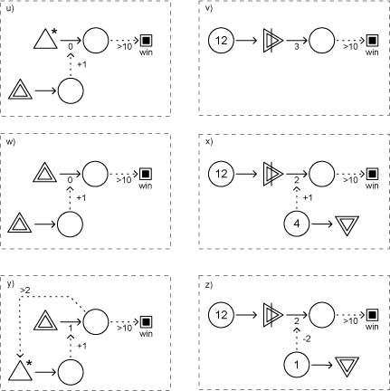
The following exercises are designed to test your familiarity with the Machinations framework and your understanding of how the tool operates. For clarity, we have drawn the diagrams so that all pools show how many resources they contain in digits, rather than in stacks.
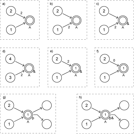
1. In each of the following eight diagrams, how many resources will be in pool A after one click?
2. In each of the following six diagrams, what is the minimum number of clicks required to move all resources to pool A?
3. In each of the following six diagrams, what is the minimum number of clicks required to move all resources to pool A?
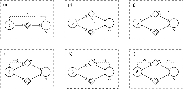
4. In each of the following six diagrams, what is the minimum number of clicks needed to win the game? Note that some diagrams have more than one interactive element.