
Chapter 8. Simulating and Balancing Games
With simple games, you can compute the odds that a given player will win without ever actually playing the game. This is commonly true of gambling games that have trivial mechanics, such as blackjack or roulette. With more complex games, especially those that include random factors, you have to play the game many times to find out whether it is fairly balanced. In several of the examples in the earlier chapters, we stated that the chance that a particular player might win or lose a game could be simulated in a digital Machinations diagram. We arrived at the number we gave based on data from thousands of simulated play tests. As you might guess, we didn’t run through all those play tests manually. The Machinations Tool allows you to define artificial players and run multiple sessions automatically to collect this type of data. These techniques are especially helpful when you are balancing your game. In this chapter, you will learn all about them.
Simulated Play Tests
As you learned in Chapter 5, “Machinations,” interactive nodes in Machinations diagrams don’t operate until the user clicks them. (Interactive nodes are drawn with a double line instead of a single one.) To simulate large numbers of play tests without human intervention, the Machinations Tool offers a special feature that can act as an artificial player. In a diagram, an artificial player is represented by a small square with the letters AP inside (Figure 8.1). It should not be connected to anything. An artificial player allows you to define a simple script to control other nodes in the diagram. This way, you can automate the actions of a player; an artificial player can “virtually click,” or activate, a node for you. (Artificial players are not limited to controlling interactive nodes, however. An artificial player can activate any named node.) While running a diagram with an artificial player, you can simply sit back and watch the action.
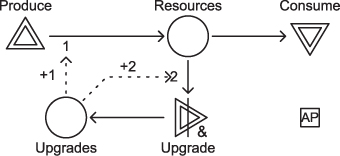
Figure 8.1. A sample diagram with an artificial player
The online Appendix C contains a detailed tutorial that shows you how to create diagrams in the Machinations Tool.
Artificial Players in Machinations
To add an artificial player to a diagram, select it from the Machinations menu and place it somewhere on the diagram. Because it doesn’t need to be connected to anything, you can put it well out of the way.
Machinations artificial-player scripts are not as powerful or complex as the scripting languages used in level design tools. You don’t need to be a programmer to create an artificial player script.
Artificial players have a number of settings that allow you to control their behavior. As with all Machinations nodes, you can set their color, line thickness, and label. An artificial player has an activation mode like any other Machinations node (see the section “Activation Modes” in Chapter 5 for more information). Most importantly, an artificial player has a script that allows you to specify what other nodes the artificial player will activate when it fires. Executing this script is an artificial player’s primary function.
Because a script stops the moment it executes a command, you cannot have two direct commands in a row in a script. The second one will never be executed. But you can have a sequence of if statements. The script will evaluate them in order until it hits one whose condition is true. It will then execute that command and stop.
A script consists of lines of instructions that tell the artificial player what to do. They may take two forms: direct commands and if statements. A direct command simply consists of an explicit order. An if statement begins with the word if followed by a condition (explained in a moment) and then a command. When an artificial player fires, it evaluates each line of its script in succession, starting at the top. If a line is a direct command, it simply executes that command. If a line is an if statement, the artificial player checks whether the given condition is true, and if so, it executes the command following the if statement. If the condition is not true, the artificial player proceeds to the next line in the script. Once any command is executed, the execution of the script stops; it does not evaluate the next line. The next time the artificial player fires, the script is evaluated again starting from the top.
Direct Commands
The most basic commands activate one or more nodes in the diagram as specified by their parameters. Once a command has executed, the script stops. All the basic commands are variations on the word fire. Node names are case sensitive.
fire(node) This command looks for a node whose label matches the parameter and fires it. For example, the command fire(Produce) will activate the source labeled Produce in Figure 8.1. The fire() command can be called without parameters. If you simply type fire() and don’t name a node within the parentheses, the script terminates and no node is fired. The same happens if the parameter of the fire() command doesn’t match any node in the diagram.
fireAll(node,node...) The fireAll() command does exactly the same thing as the fire() command, but it accepts more than one parameter. When executed, it fires all the named nodes simultaneously.
fireSequence(node,node...) The fireSequence() command is rather specialized: It activates the nodes listed in its parameters one at a time in order, changing to the next node each time the command is executed. The first time the script executes fireSequence(), it will activate the first node in the parameter list. The second time the script executes fireSequence(), it will activate the second node in the list, and so on. It automatically keeps track of which one is next. If the command is executed more times than it has parameters, it will simply start again from the first parameter. For example, the command fireSequence(Produce, Produce, Upgrade, Produce, Consume) will cycle through activating the source twice, the converter, the source again, and then the drain in Figure 8.1.
fireRandom(node,node...) This command takes as parameters the names of multiple nodes, but it selects one of them at random and fires it. To increase the probability of it firing a given node, you can enter that node’s name more than once. For example, in Figure 8.1, the command fireRandom(Produce, Produce, Consume, Upgrade) has a 50% chance of activating the source, a 25% chance of firing the drain, and a 25% chance of firing the converter.
If Statements
The script of an artificial player also lets you specify conditional commands using if statements. if statements consist of the word if, a condition specified in parentheses, and a command to execute if the condition is true.
if(condition)command The condition in an if statement can refer to pools and registers to check the state of the diagram. For example, the script line if(Resources>3) fire(Consume) activates the drain in Figure 8.1 when there are more than three resources in the pool labeled Resources.
There is no need for an else statement in the scripts for artificial players because the script executes until it finds either an if statement that is true or one of the direct commands. For example, the following script will fill the pool marked Resources in Figure 8.1 with a few resources before randomly choosing between a Consume or Upgrade action:
if(Resources>4) fireRandom(Consume, Upgrade)
fire(Produce)
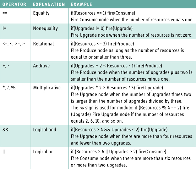
An if statement allows you to perform calculations and string multiple conditions together with logical operators. It works the way you would expect if you are already familiar with if statements in programming languages like Java or C. Table 8.1 lists the possible operators supported by the conditions in an if statement.
Table 8.1. Possible Operators in Script Conditions
Extra Commands
Apart from the various kinds of fire commands, there are a few extra commands you can use in a script for an artificial player:
stopDiagram(message)
Stops the execution of the diagram immediately, very much like an end condition does. You can put a string of text in the parameter. If you have more than one artificial player, you might want to use a different message in the script of each player to let you know which player stopped the diagram. When executing multiple runs (see “Collecting Data from Multiple Runs”), the tool will keep track of how many times each message appeared and let you know in a dialog box as the runs take place. This will enable you to collect statistics on what causes a diagram to stop.
• endTurn() Ends the current turn in a turn-based diagram.
• activate(parameter) Deactivates the current artificial player and activates the one identified by the parameter instead.
• deactivate() Deactivates the artificial player.
When a diagram uses color-coding, the artificial players may be color-coded as well. In that case, an artificial player can fire only nodes that are the same color as itself.
Artificial players can also be used in a turn-based diagram (see the section “Time Modes” in Chapter 5 for a discussion of turn-based diagrams). However, in that case, their behavior changes a little. Most importantly, in a turn-based diagram, the artificial player has a number of actions that indicate how many times it will fire during a turn. When it has multiple actions per turn, these actions are executed at one-second intervals.
Collecting Data from Multiple Runs
Artificial players allow you to run diagrams and test games automatically. To make the best use of this option, the Machinations Tool allows you to quick run the diagram (Figure 8.2). You do this by switching to the Run tab in the tool and clicking the Quick Run button. While quick running, the diagram executes very quickly but doesn’t allow any interaction. If you are using quick run, you must make sure that the diagram has an end condition and can actually reach that end condition. If the diagram keeps on running without reaching an end condition, you can click the Quick Run button again (which is now labeled Stop) to stop it manually. Click the same button once more to reset the diagram back to its starting condition.
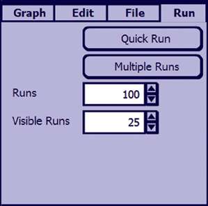
Figure 8.2. The Run panel of the Machinations Tool
You also have the option to run a diagram multiple times. To do this, go to the Run tab in the Machinations Tool and click the Multiple Runs button. By default, the number of times that a diagram runs is set to 100, but you can easily change this number in the Run tab. To prevent the tool from running endlessly, if a running diagram in a multiple run batch doesn’t reach an end condition after 10,000 time steps, it will stop automatically. When running multiple times, the diagram will keep track of the number of times that each of its end conditions were reached. If you have a game with two players that each have their own win condition (which would be an end condition also), this makes it easy to determine who wins more often. This feature was used to create the statistical data given in some of the examples in this book. When you run a diagram multiple times, the diagram also keeps track of the elapsed time of each run and lets you know the overall average, which can be useful when comparing different artificial player scripts to see which script drives the economy toward a particular state (normally victory!) the fastest.
Finally, if your diagram contains a chart, the data from each run is stored in the chart (Figure 8.3). By default, charts display the data from the last 25 runs, but they store more. You can actually browse through all the data captured by the chart by clicking the << and >> symbols below the chart. The data from the current run will be bright while the other runs are dim. (Figure 8.3 is currently showing the results from the 97th run.) To clear a chart’s data between simulations, click the word clear on the chart. You can also save the collected data as a comma-separated values data file (*.csv) for further analysis in a spreadsheet or statistics program. To do this, click the word export below the chart and choose a location to save the file.
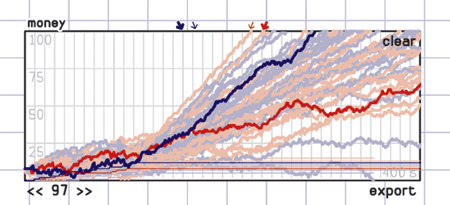
Figure 8.3. A Machinations chart showing the result of 100 runs
Designing Artificial Player Strategies
Artificial players cannot replace real players, and the scripting options will not allow you to create clever artificial intelligence (AI). The purpose of artificial players is to test relatively simple strategies to see how the mechanics operate, not to build an adaptive AI player. To get the most out of artificial players and automated play tests, it is best to design artificial players that represent caricatures: Design them to consistently follow a particular strategy, no matter the consequences. For example, if you want to find out what mix of unit types is best for a real-time strategy game, design a few different artificial players to build the various mixes that you want to try and have them play each other. Artificial players can be passive or automatic just like any other node. This allows you to switch between different artificial players quickly and thus try different artificial players simultaneously. While you are running a diagram, you can click an artificial player to switch it between automatic and passive modes.
It often takes several tries to get the strategy for an artificial player right. This is to be expected, especially if you are creating artificial players for your own designs. Designing artificial players is a good way to explore and test your design. Ideally, you should be able to find many valid strategies for your artificial players to follow. If you can script an artificial player that consistently beats other artificial players (or yourself), you probably have found a dominant strategy, and you need to change the mechanics to reduce the effectiveness of that strategy.
Removing All Randomness
As we discussed in the section “Randomness vs. Emergence” in Chapter 6, “Common Mechanisms,” random factors can obscure the operation of a pattern that might create a dominant strategy. When testing for balance, it is important to identify dominant strategies, and this will be easier to do if you remove the random factors from the mechanics.
Randomness that is expressed as a percentage in a Machinations diagram can be easily replaced by substituting a fraction representing the average value. If you have a source that randomly produces resources with a probability of 20%, you can replace this number with a fixed production rate of 0.2. This will cause the source to produce a resource at the rate of two every ten time steps. Randomness that is expressed as a range generated by rolling multiple dice (such as 3D6) is more difficult to replace because the probability distribution is not uniform. We suggest using the average. The formula for the average with any number of dice that all have the same number of sides is as follows:
Average die roll = (Number of sides on a die +1) × Number of dice ÷ 2
In the case of 3D6, it is (6+1) × 3 ÷ 2, or 10.5.
Alternatively, you might want to make sure that the script of your artificial players does not involve any randomness. In this case, replace all fireRandom() commands with fireSequential() commands and find a different value for all conditions that involve random. For example, if(random < 0.3) fireRandom(A, B, B, C) could be rewritten as if(steps % 10 < 3) fireSequential(A, B, B, C).
If you remove all the randomness in labels on connectors and all the randomness appearing in artificial player scripts, you will always get the same result from running the diagram. This might be a good way to find out whether a certain strategy is actually superior to another strategy.
Linking Artificial Players
When working with artificial players, your scripts can get long and complex. One way to reduce the complexity of the scripts is to split a script over multiple artificial players. This can be done by having one artificial player firing another, interactive artificial player. For example, you could create one artificial player called builder that you design to identify and fire the best building action, while you create another called attacker to identify and fire the best offensive actions. In that case, you could randomly select between the two by creating a third artificial player with the script fireRandom(builder, attacker).
A word of caution, however: Artificial players allow you more control over the behavior of a Machinations diagram, but this can cause you to mislead yourself about how well-balanced or manageable your economy is. If you have to spend a lot of time trying to make artificial players that successfully control your economy, that’s usually an indication that your economy has a problem. Artificial players aren’t supposed to be smart enough to beat a game that is unfair to the player or has other weaknesses. Their purpose is to reveal issues, not to obscure them. Tune your mechanics, not your artificial players.
Playing with Monopoly
For our first detailed example of an automated Machinations diagram, we will explore the balance of the game Monopoly. We’ll look at how this balance is affected by the different mechanisms in the game and how design patterns might be applied to improve the game.
Figure 8.4 represents a model of Monopoly. It is slightly different from the models we have used for Monopoly so far. The important differences are as follows:
• It represents a two-player game. Earlier in the book we used a source and a drain to represent the player receiving and paying rent, but this has been replaced by two gates that transfer money between the two players. In this case, every property that a player has generates a 4% chance that the other player has to pay one money unit every time step.
• The number of available properties is limited. In this example, there are only 20 properties in the game initially stored in the Available pool. Once they are gone, the players cannot buy more property.
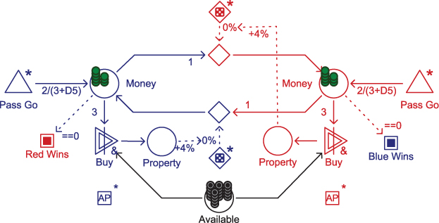
Figure 8.4. A two-player version of Monopoly
We also defined two artificial players that control each player. Both artificial players have a simple, single-line script. This script reads as follows:
if((random * 10 < 1) && (Money > 4 + steps * 0.04)) fire(Buy)
The effect is that each artificial player has a 10% chance that it will buy a property in each time step. It will buy property only if it has enough money, however. Initially the player must have more than four money units in its pool in order to buy, but this value gradually increases as the game progresses (this is why the steps value appears in the condition). This condition was added to make sure the artificial player did not exhaust its money too quickly and lose the game early on. We set it up so that the minimum amount of money the artificial player keeps in its pool gradually increases, because as more property is bought by each player, the chances increase that the player will have to pay more rent on consecutive turns. It needs to keep a larger and larger reserve as time goes on.
Simulated Play-Test Analysis
Running these identical players against each other and tracking the amount of money that each player has over multiple sessions produces a chart like the one in Figure 8.5. Reading this chart is not easy, but a few features do stand out. The amount of money that both players have stays more or less stable for the first 90 steps or so but then starts to increase gradually. Figure 8.6 highlights this trend. (We added the Trend line for illustration; it was not generated by the Machinations Tool.) As we discussed in previous chapters, this trend is the result of the positive feedback that is at the heart of Monopoly. More importantly, it is typical of the dynamic engine pattern discussed in Chapter 7, “Design Patterns” (see also Appendix B).
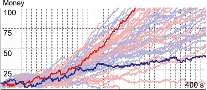
Figure 8.5. Multiple sessions of simulated play. The brighter lines are the most recent run.
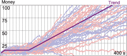
Figure 8.6. The trend in the gameplay
To better study this trend, we can remove all randomness from the diagram. This is done by changing the production rates, the implementation of the rent mechanism, and the script of the artificial players. Figure 8.7 reflects these changes. The new script for the deterministic artificial players is as follows:
if((steps % 10 < 1) && (Money > 4 + steps * 0.04)) fire(Buy)
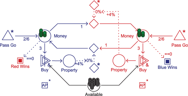
Figure 8.7. A deterministic version of Monopoly
You can see the result of simulated play session in Figure 8.8. The trend is very clear in this chart. (Note that in this chart the two players completely overlap because they are following identical strategies, so only one player is visible.) Also note that in this chart the number of properties owned by each player is represented as a thin line.
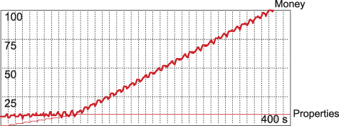
Figure 8.8. A simulated play session of deterministic Monopoly
The Effects of Luck
To study the effects of luck on the game of Monopoly, we then changed the script of the red player to read as follows:
if((steps % 20 < 1) && (Money > 4 + steps * 0.02)) fire(Buy)
This leads to a situation in which the red player has only half as many opportunities to buy a new property. Instead of buying every 10 steps, red buys only every 20 steps. Figure 8.9 displays a chart that reflects these changes. If you look only at the money lines, the players’ fortunes don’t seem that different initially. However, as any experienced player of Monopoly will tell you, the game is all about getting the properties. The difference in properties held is the real indication of the players’ strengths.
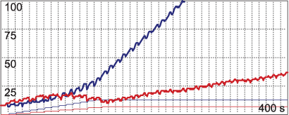
Figure 8.9. The effect of a consistent difference in luck. Thick lines are money owned; thin lines are properties owned.
Using this chart, we can study the effects of randomizing various mechanics. For example, Figure 8.10 illustrates the effects of randomizing the time it takes to pass Go again (by restoring the production rate of that pool to 2/(3+D5), thus 2 every 4 to 8 turns). As you can see, the effects are not that great. Most importantly, it does not affect the main trend of the game very much. Passing Go doesn’t really influence the game significantly.
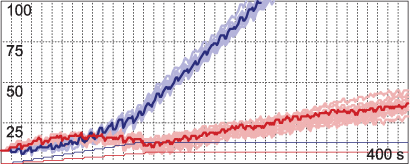
Figure 8.10. The effect of randomizing how often the players pass Go
The effects of randomizing the rent mechanism, as shown by Figure 8.11, are greater. Even so, it does not break the general trend (although if you look at the chart carefully, you might notice that it sometimes results in red having much less money and therefore being able to buy fewer properties).
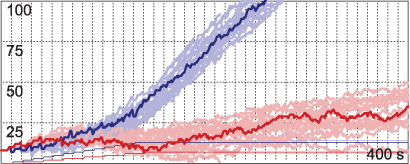
Figure 8.11. The effect of randomizing the rent mechanism
However, randomizing the chance that a player gets the opportunity to buy property has a far greater effect (Figure 8.12). Most importantly, it affects the distribution of properties between players and impacts the money distribution as a result. To implement the different opportunities, the script for the blue player reads as follows:
if((random * 10 < 1) && (Money > 4 + steps * 0.02)) fire(Buy)
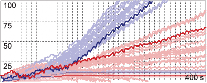
Figure 8.12. The effect of randomizing the opportunity to buy property
While the script for the red player reads as follows:
if((random * 20 < 1) && (Money > 4 + steps * 0.02)) fire(Buy)
If we put all these effects in a single diagram, the chart looks like the one in Figure 8.13. Note, however, that this chart is different from the first chart of Monopoly (Figure 8.5), because in this chart the odds are still against the red player. He has about half as many opportunities to buy a property as the blue player. Also note that although the fortunes of both players are more varied, red rarely wins.

Figure 8.13. All mechanics randomized
Rent and Income Balance
One problem with our model of Monopoly is that in most runs the game doesn’t end in victory for one player, so the Machinations Tool stops the simulation after a while. One player might get rich because he takes more rent from the other player, but as long as the other player can compensate for it by passing Go frequently enough, the game goes on indefinitely. This is because, so far, our model hasn’t implemented the rent inflation that is built into the real game. Houses and hotels are a critically important part of Monopoly. They allow the player to invest in his properties, which increases the rent if another player ends a turn on his property. Figure 8.14 adds this mechanism to the game. In this diagram, players can buy both properties and houses, which increases their chance to get a bigger payout when receiving rent.
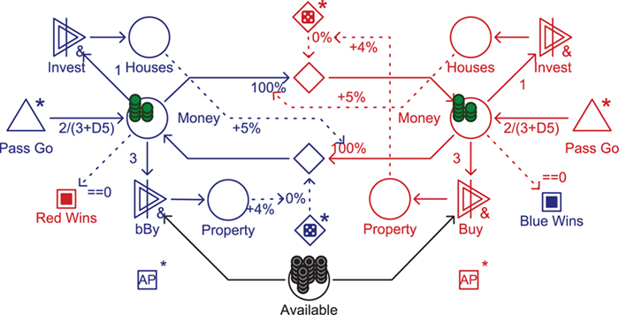
Figure 8.14. Monopoly with an additional mechanism to buy houses
To allow the artificial players to use the new gameplay option, we used the following script:
if((random * 10 < 1) && (Money > 4 + steps * 0.04)) fire(Buy)
if((Property > Houses / 5) && Money > 6 + steps * 0.04)) fire(Invest)
The first line of the script is just the same as it was: The player has a random 10% chance of buying a property every time step, if he has enough money saved. The second line states that if he has more than five times as many properties as houses (and even more money saved), then he invests in a house.
The best way to see the effect of this balance is to turn the diagram into a deterministic version (removing all random factors), increase the income from passing Go, and have one artificial player invest in houses and the other not. Without the option to invest in houses, both players enjoy an identical steady increase of money, as shown by the purple line in Figure 8.15. But if one player does invest (blue) while the other does not (red), the one who invests will win.
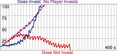
Figure 8.15. The effects of investing in houses
What we’ve done here is to change the balance between income from passing Go and costs from paying rent. It’s no longer possible to pass Go enough to cover the rising rent—even if we set the amount earned by passing Go fairly high. We ran a nondeterministic diagram 1,000 times in which both players invest in houses, with an income from Go set to 5/(3+D5). We learned that somebody will win the game roughly 75% of the time (with an equal chance of either player winning). The other 25% of the time the game drags on until the Machinations Tool stops it. But with income set to 2/(3+D5), the chances of a game dragging on forever drop to zero. With a high income and the effects of rent inflation doubled, the chance of entering an equilibrium is reduced to 2%. The graphs these settings produce in general look quite interesting (Figure 8.16).
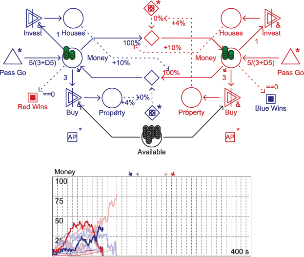
Figure 8.16. A better balance between rent and income
Adding Dynamic Friction
Our model of Monopoly has now added rent inflation and solved the early problem that passing Go permitted the game to go on forever. However, the power of property is now actually too high. Having more property than your opponent is the most significant indicator of who is going to win. This means that the dynamic engine pattern in the game is too dominant. Looking through the design patterns in Appendix B suggests a solution: By applying dynamic friction, the positive feedback might be kept in check.
We can easily introduce dynamic friction by adding a form of property tax (and indeed property tax, in a different form, does exist in the board game). At certain intervals, the player loses money based on the number of properties and/or houses she has. The new construction is represented in Figure 8.17. The new property tax mechanism, a drain off each player’s Money pool, is shown with thick lines. It drains some money (initially set to zero) every six time steps. The amount that it drains goes up as the player collects property and houses; this is controlled by thick-lined state connections (dotted lines) from the player’s Houses and Property pools to the label on the resource connection leading to the Property Tax drain. The tax rate shown in the diagram is 6% per house and 30% per property.
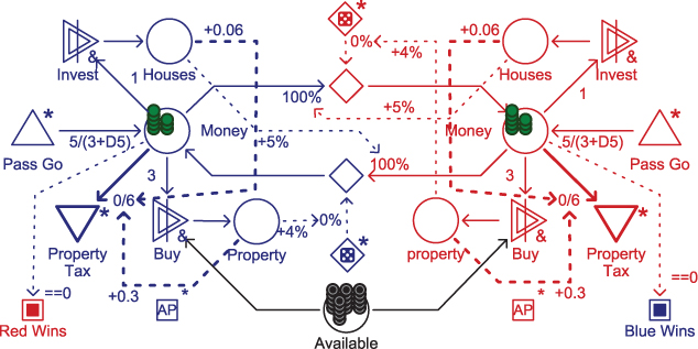
Figure 8.17. Monopoly with a property tax mechanism
Table 8.2 lists the statistics gathered from simulating the game 1,000 times with different settings for the property tax. Blue was programmed to buy 14 properties, and red to buy 6. The table exhibits a couple of interesting features. With no taxes, blue has a clear advantage produced by his larger number of properties. As tax rates go up, however, blue’s advantage decreases. Greater than a certain point, the taxes are so high that blue’s properties are actually a disadvantage to his economic success, and blue starts to lose more often than he wins. Set correctly, the taxes do indeed act as dynamic friction, reducing the effect of positive feedback.
Table 8.2. Effects of Different Property Tax Rate Settings
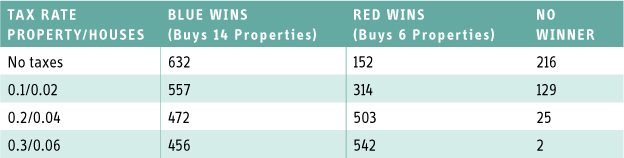
Both artificial players are set to purchase property and houses at the earliest available opportunity, which might not be the best strategy if property taxes are in operation. They might do better if they played a bit more conservatively.
Another thing to notice in the table is that the property taxes reduce the number of “no winner” outcomes. This, too, is a desirable quality in a game: The friction helps prevent stalemates.
Balancing SimWar
So far, all the extended examples in this book have been about games that have already been published. But the Machinations framework is not just a tool for analysis. To demonstrate the framework’s value for designing new games, we will discuss in detail a game that (to our knowledge) never has been built yet is known to game design community. This game is SimWar.
SimWar was presented during the Game Developers’ Conference in 2003 by game designer Will Wright, who is well-known for his published simulation games, SimCity and The Sims, among many others. SimWar is a hypothetical, minimalistic war game that features only three units: factories, immobile defensive units, and mobile offensive units. These units can be built by spending an unspecified resource that is produced by factories. The more factories a player has, the more resources become available to build new units. Only offensive units can move around the map. When an offensive unit meets an enemy defensive unit there is a 50% chance that one destroys the other, and vice versa. Figure 8.18 is a visual summary of the game and includes the respective building costs of the three units.
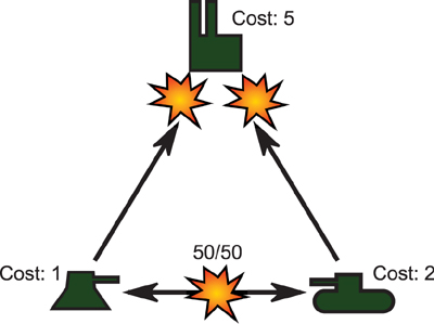
Figure 8.18. A visual summary of SimWar (Wright, 2003)
During his presentation, Wright argued that this minimal real-time strategy game still presents the player with some interesting choices and displays dynamic behavior similar to that found in other games within the same genre. Most notably Wright argued that a rock-paper-scissors mechanism affects the three units: Building factories trumps building defenses, building defenses trumps building offensive units, and building offensive units trumps building factories. Wright also describes a short-term vs. long-term trade-off and a high-risk/high-reward strategy that recalls the “rush” and “turtle” strategies found in many real-time strategy games (see the sidebar “Turtling vs. Rushing”).
Modeling SimWar
In this section, we build a model of SimWar in stages, using Machinations diagrams. The mechanics we build in each stage follow the same structure as the ones we offered as real-time strategy examples in Chapter 6.
Starting with the production mechanism, we use a pool (Resources) to represent a player’s collected resources (Figure 8.19). The pool is filled by another automatic pool that represents the uncollected resources available to the player. The game’s production rate is initially 0 but increases by 0.25 for every factory the player builds. The player can build factories by clicking the interactive converter labeled BuildF, which will pull resources only when at least five are available. The structure is a typical implementation of the dynamic engine pattern that we discussed in Chapter 7. Like all dynamic engines, it creates a positive feedback loop: The more factories a player builds, the quicker resources are produced, which in turn can be used to build even more factories. However, as the resources are ultimately limited, building only factories might not be the best idea. Notice that, in this case, the structure requires players to start with at least five resources already collected or one factory already built. Otherwise, players can never start producing.
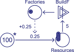
Figure 8.19. Factories produce resources.
Resources are also used to build offensive and defensive units. Figure 8.20 illustrates the mechanics for this. The diagram uses color-coded resources. The units produced by the converter labeled BuildD are blue, while the units produced by BuildO are green as indicated by the color of their respective outputs. This means that blue resources (representing defensive units) and green resources (representing offensive units) are both gathered on the Defense pool. However, clicking the Attack pool will pull all green resources toward it. This way, only offensive units can be used to launch an attack.
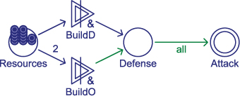
Figure 8.20. Spending resources to build offensive and defensive units
Figure 8.21 illustrates how combat between two players is modeled. In each time step, each attacking unit of one player has a chance to destroy a defending unit of the other player, and similarly, defending units have a chance to destroy attacking units. Attacking units also have a chance to destroy enemy factories, but that drain is active only when the defending player has no defending units left.
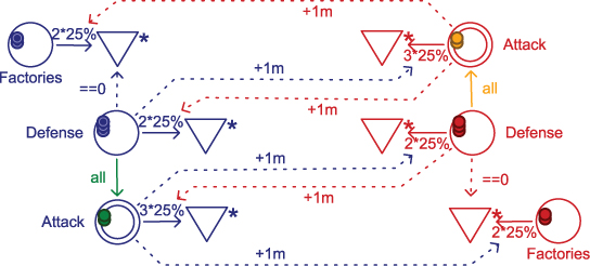
Figure 8.21. Attacking and defending
Putting It All Together
Combining the structures of each step, we have a model for a two-player version of SimWar (Figure 8.22). One player controls the blue (defensive) and green (offensive) elements on the left side of the diagram, while the other player controls the red (defensive) and orange (offensive) elements on the right side of the diagram. The two sides are symmetrical.
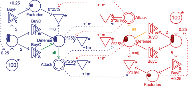
Figure 8.22. Two-player version of SimWar
Figure 8.23 displays the relative strength of each player as it developed over time during a simulated session. We chose an arbitrary definition of strength: We gave five points for each factory owned, plus one for each defensive unit, one for each offensive unit in reserve, and two for each offensive unit currently attacking. The chart displays what looks like an interesting and close match. This might suggest a balanced game, but because both artificial players were following the same strategy, we cannot jump to that conclusion.
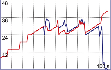
Figure 8.23. Two players playing
Defining Artificial Players
If you are looking for a challenge yourself, try to beat our artificial player called random turtle in a simulated game of SimWar. You can find it on the companion website (see the “Playing SimWar on the Companion Website” sidebar). This player follows a turtling strategy: It builds up its defense and factories before building offensive units and launching attacks. Its behavior is determined by the following script:
if(Defense <= 3 + pregen0 * 3) do(BuyD)
if(Factories <= 2 + pregen1 * 3) do(BuyF)
if(Defense > 6 + pregen2 * 3 && random < 0.2) do(Attack)
if(Resources > pregen3 * 4) do(BuyO)
Note that this script uses the pregenerated random values (pregen0—pregen3) in order to alter its strategies a little every time the simulation runs. It will build between four and six defensive units first, then build between three and five factories, before focusing on the attack.
Fun as it may be to play against the “random turtle” strategy or investigate the data from having two of those artificial players face each other, it reveals little of the balance of the game. Most strategy games allow for rushing and turtling strategies. The following script defines our turtling strategy:
if(Defense < 4) fire(BuyD)
if(Factories < 4) fire(BuyF)
if(Defense > 9 && random < 0.2) fire(Attack)
if(Resources > 3) fire(BuyO)
Our turtle strategy gives priority to building four defensive units and four factories first. After that, it starts building offensive units and starts attacking if it has a total of ten or more units.
The following script defines our rushing strategy:
if(Defense < 3) fire(BuyD)
if(Factories < 2) fire(BuyF)
if(Defense > 5 + steps * 0.05 && random<0.2) fire(Attack)
if(Resources > 1) fire(BuyO)
This script puts far less priority on building factories and defenses. It buys two defenses and then one factory and then starts producing offensive units. Initially it will try to launch waves quickly, but as time progresses, it tries to save up for bigger assaults.
Note that, apart from the random factor used to time attacks, the scripts define very consistent strategies. The artificial players will always follow the same strategy, whether it is successful or not. Because their behavior is consistent, they are ideal to determine which strategy is more effective, rushing or turtling. A thousand simulated runs reveal that the turtling strategy is superior by far: It wins roughly 92% of the time. What’s more, a large proportion of the wins for the rushing player are the result of the turtling player running out of resources—which doesn’t occur very often.
Each row gives the results from 1,000 runs, done automatically. However, the process of changing the tweaks required manually adjusting the diagram.
Tweaking the Balance
Clearly, turtling is too successful in our model of SimWar. To find a better balance, we can try to tweak several values. We’ll start with changing the production costs for each unit type. You can find the results for 1,000 simulated runs for each tweak in Table 8.3.
Table 8.3. Effects of Tweaking Production Costs in SimWar
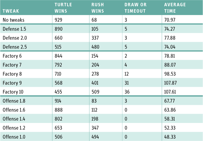
Surprisingly, these tests show us that increasing the cost for defensive units has little impact on the balance between rushing and turtling strategies. Only when a defensive unit costs more than an offensive unit, making it a really poor choice, does the turtle strategy start to lose more frequently than the rushing strategy does. This leads to the conclusion that the balance between rushing and turtling strategy is mostly affected by the balance between production and offensive units and little by the balance between offensive and defensive units. Also notice that increasing the factory costs initially increases the average game length, but it stabilizes when a factory costs eight or more units. This can be explained by the fact that increasing the factory cost slows the game down because it takes more time to build up production capacity. At the same time, a very high factory cost favors the rushing strategy, which tends to win faster than the turtling strategy. At high factory costs, the second effect dominates the first effect.
We can also change the balance between the costs of factories and the costs of units by increasing or reducing their effects. In this case, we tried different variables for the factories’ production rates (the number of resources each factory produces) and the chance that attacking units will destroy defensive ones. We also tried different settings for the initial and total available resources. Table 8.4 lists the effects of these tweaks.
Table 8.4. Effects of Various Tweaks on the Balance of SimWar
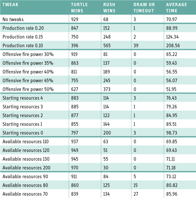
The best balance is probably found by applying a combination of these tweaks. For example, keeping an eye on the average playing time, we opted to reduce the production rate to 0.20, the factory cost to 7, and the offensive power to 35%. With these mechanics, the two strategies are evenly balanced (in the test run, each won exactly 500 times!) against an average playing time of 83.02 time steps.
From Model to Game
Balancing a Machinations diagram is a useful exercise, but it doesn’t guarantee that the game you are working on will automatically be balanced as well. A Machinations diagram represents an abstract perspective on your game. It lacks detail, and as a result, your real game might behave a little differently. When you balance a Machinations diagram, you should be aware of these differences. The closer your game design is to the Machinations diagram, the more likely it is that your balancing efforts in the Machinations Tool will translate directly to the game. But remember that Machinations cannot account for peculiarities of human player behavior (such as bluffing) or the effects of strategic maneuvering in a war game.
However, playing with the balance of a diagram is usually worth the effort, even if the balance does not translate directly. By spending some time balancing the diagram, you are gaining insights into balancing the real game. As long as the structure of the diagram matches the structure of the mechanics, you can expect that certain effects will be similar. For example, finding out that the relative costs of factories and offensive units in SimWar has a great impact on the balance between turtling and rushing strategies will help you when you are looking for the right balance in a full implementation of the game. By running play tests on the diagram, you are likely to recognize gameplay patterns that will emerge from play testing the full game.
Summary
To balance a game, you must play test it many times, and this can be difficult with long and complex games. The Machinations Tool lets you simulate play tests rapidly by creating artificial players that execute simple strategies automatically. You can run hundreds of play tests in a few seconds and collect statistical data to show whether your game is balanced and how well different strategies work.
Monopoly, as always, serves as a good game to analyze. In this chapter, we built a model of Monopoly that included buying properties and houses and showed how different purchasing strategies changed the balance of the game. We also demonstrated how to reduce the effect of strong positive feedback produced by the dynamic engine pattern that generates income from rent by introducing a dynamic friction pattern as well. For our example, we used a tax on houses and properties.
To end the chapter, we modeled Will Wright’s hypothetical game SimWar and showed how tweaking its various features over many simulated play tests resulted in differing levels of success for two player strategies, rushing and turtling. This is exactly the sort of testing you have to do when designing a new internal economy for a game, which demonstrates the value of Machinations to professional game design.
Exercises
1. Change the mechanics of Monopoly (the real board game) so that the game ends sooner and is better balanced than the original.
2. Define artificial player strategies for Monopoly that reflect a different preference for buying houses and buying properties, without altering the chances of getting an opportunity to buy. Can you find one that has a significantly better chance to beat the artificial player used in our experiments?
3. Hold a competition to find out who can build the best artificial player for SimWar. You may add multiple artificial players that control one another, but you may not change the basic structure of the diagram. Alternatively, use the better balanced settings (production rate 0.20, factory cost 7, offensive fire power 35%) for this competition.
4. Investigate how different building times for the units in SimWar affect the balance of that game.