Stitching Tables Together

Joining is the defining functionality of SQL and sets it apart from other data technologies. Be sure you are somewhat comfortable with the material we’ve covered so far, and take your time practicing and reviewing before moving on.

Let’s rewind back to the beginning of this book, when we were discussing relational databases. Remember how “normalized” databases often have tables with fields that point to other tables? For example, consider this CUSTOMER_ORDER table, which has a CUSTOMER_ID field (Figure 8-1).

Figure 8-1. The CUSTOMER_ORDER table has a CUSTOMER_ID field

This CUSTOMER_ID field gives us a key to look up in the table CUSTOMER. Knowing this, it should be no surprise that the CUSTOMER table also has a CUSTOMER_ID field (Figure 8-2).

Figure 8-2. The CUSTOMER table has a CUSTOMER_ID key field that can be used to get customer information

We can retrieve customer information for an order from this table, very much like a VLOOKUP in Excel.

This is an example of a relationship between the CUSTOMER_ORDER table and the CUSTOMER table. We can say  that CUSTOMER is a parent to CUSTOMER_ORDER. Because CUSTOMER_ORDER depends on CUSTOMER for information, it is a child of CUSTOMER. Conversely, CUSTOMER cannot be a child of CUSTOMER_ORDER because it does not rely on it for any information.  The diagram in Figure 8-3 shows this relationship; the arrow shows that CUSTOMER supplies customer information to CUSTOMER_ORDER via the CUSTOMER_ID.

Figure 8-3. CUSTOMER is the parent to CUSTOMER_ORDER, because CUSTOMER_ORDER depends on it for CUSTOMER information

The other aspect to consider in a relationship is how many records in the child can be tied to a single record of the parent. Take the CUSTOMER and CUSTOMER_ORDER tables and you will  see it is a one-to-many relationship, where a single customer record can line up with multiple orders. Let’s take a look at Figure 8-4 to see a specific example: the customer “Re-Barre Construction” with CUSTOMER_ID 3 is tied to three orders.

Figure 8-4. A one-to-many relationship between CUSTOMER and CUSTOMER_ORDER

One-to-many is the most common type of relationship because it accommodates most business needs, such as a single customer having multiple orders. Business data in a well-designed database should strive for a one-to-many pattern. Less common are the one-to-one and many-to-many relationships (sometimes referred to as a Cartesian product). These are worth researching later, but in the interest of focusing the scope of this book, we will steer clear of them.

INNER JOIN

Understanding table relationships, we can consider that it might be nice to stitch two tables together, so we can see CUSTOMER and CUSTOMER_ORDER information alongside each other. Otherwise, we will have to manually perform tons of lookups with CUSTOMER_ID, which can be quite tedious. We can avoid that with JOIN operators, and we will start by learning the INNER JOIN.

The INNER JOIN allows us to merge two tables together. But if we are going to merge tables, we need to define a commonality between the two so records from both tables line up. We need to define one or more fields they have in common and join on them. If we are going to query the CUSTOMER_ORDER table and join it to CUSTOMER to bring in customer information, we need to define the commonality on CUSTOMER_ID.

Open up the rexon_metals database and open a new SQL editor window. We are going to execute our first INNER JOIN:

SELECT ORDER_ID,
CUSTOMER.CUSTOMER_ID,
ORDER_DATE,
SHIP_DATE,
NAME,
STREET_ADDRESS,
CITY,
STATE,
ZIP,
PRODUCT_ID,
ORDER_QTY

FROM CUSTOMER INNER JOIN CUSTOMER_ORDER
ON CUSTOMER.CUSTOMER_ID = CUSTOMER_ORDER.CUSTOMER_ID

The first thing you may notice is we were able to query fields from both CUSTOMER and CUSTOMER_ORDER. It is almost like we took those two tables and temporarily merged them into a single table, which we queried off of. In effect, that is exactly what we did!

Let’s break down how this was accomplished. First, we select the fields we want from the CUSTOMER and CUSTOMER_ORDER tables:

SELECT CUSTOMER.CUSTOMER_ID,
NAME,
STREET_ADDRESS,
CITY,
STATE,
ZIP,
ORDER_DATE,
SHIP_DATE,
ORDER_ID,
PRODUCT_ID,
ORDER_QTY

FROM CUSTOMER INNER JOIN CUSTOMER_ORDER
ON CUSTOMER.CUSTOMER_ID = CUSTOMER_ORDER.CUSTOMER_ID

In this case, we want to show customer address information for each order. Also notice that because CUSTOMER_ID is in both tables, we had to explicitly choose one (although it should not matter which). In this case, we chose the CUSTOMER_ID in CUSTOMER using an explicit syntax, CUSTOMER.CUSTOMER_ID.

Finally, the important part that temporarily merges two tables into one. The FROM statement is where we execute our INNER JOIN. We specify that we are pulling from CUSTOMER and inner joining it with CUSTOMER_ORDER, and that the commonality is on the CUSTOMER_ID fields (which have to be equal to line up):

SELECT CUSTOMER.CUSTOMER_ID,
NAME,
STREET_ADDRESS,
CITY,
STATE,
ZIP,
ORDER_DATE,
SHIP_DATE,
ORDER_ID,
PRODUCT_ID,
ORDER_QTY

FROM CUSTOMER INNER JOIN CUSTOMER_ORDER
ON CUSTOMER.CUSTOMER_ID = CUSTOMER_ORDER.CUSTOMER_ID

If you have worked with Excel, think of this as a VLOOKUP on steroids, where instead of looking up CUSTOMER_ID and getting one value from another table, we are getting the entire matching record. This enables us to select any number of fields from the other table.

Now take a look at the results (Figure 8-5). Thanks to the INNER JOIN, this query gives us a view that includes the customer details with each order.

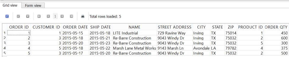
Figure 8-5. CUSTOMER inner joined with CUSTOMER_ORDER

Joins truly give us the best of both worlds. We store data efficiently through normalization, but can use joins to merge tables together on common fields to create more descriptive views of the data.

There is one behavior with INNER JOIN to be aware of. Take a moment to look at the results of the preceding query. We can see that we have three “Re-Barre Construction” orders, as well as an order from “LITE Industrial” and another from “Marsh Lane Metal Works.” But are we missing anybody?

If you go look at the CUSTOMER table, you will see there are five customers. Our INNER JOIN query captured only three. “Rex Tooling Inc” and “Prairie Construction” are nowhere to be found in our query results. So what exactly happened? There are no orders for Rex Tooling Inc and Prairie Construction, and because of this the INNER JOIN excluded them from the query. It will only show records that inclusively exist in both tables (Figure 8-6).

Figure 8-6. A visualized inner join between CUSTOMER and CUSTOMER_ORDER (note the two customers getting omitted, as they have no orders to join to)

With an INNER JOIN, any records that do not have a common joined value in both tables will be excluded. If we want to include all records from the CUSTOMER table, we can accomplish this with a LEFT JOIN.

LEFT JOIN

Those two customers, Rex Tooling Inc and Prairie Construction, were excluded from the INNER JOIN on CUSTOMER_ID because they had no orders to join on. But suppose we did want to include them anyway. Often, we may want to join tables and see, for example, all customers, even if they had no orders.

If you are comfortable with the INNER JOIN, the left outer join is not much different. But there is one very subtle difference. Modify your query from before and replace the INNER JOIN with LEFT JOIN, the keywords for a left outer join. As shown in Figure 8-7, the table specified on the “left” side of the LEFT JOIN operator (CUSTOMER) will have all its records included, even if they do not have any child records in the “right” table (CUSTOMER_ORDER).

Figure 8-7. The LEFT JOIN will include all records on the “left” table, even if they have nothing to join to on the “right” table (which will be null)

Running this, we have similar results to what we got from the INNER JOIN query earlier, but we have two additional records for the customers that have no orders (Figure 8-8). For those two customers, notice all the fields that come from CUSTOMER_ORDER are null, because there were no orders to join to. Instead of omitting them like the INNER JOIN did, the LEFT JOIN just made them null (Figure 8-9).

Figure 8-8. CUSTOMER left joined with CUSTOMER_ORDER (note the null CUSTOMER_ORDER fields mean no orders were found for those two customers)

Figure 8-9. CUSTOMER left joined with CUSTOMER_ORDER (note that “Rex Tooling” and “Prairie Construction” joined to NULL, as they have no orders to join to)

It is also common to use LEFT JOIN to check for “orphaned” child records that have no parent, or conversely a parent that has no children (e.g., orders that have no customers, or customers that have no orders). You can use a WHERE statement to check for null values that are a result of the LEFT JOIN. Modifying our previous example, we can filter for customers that have no orders by filtering any field from the right table that is null:

SELECT
CUSTOMER.CUSTOMER_ID,
NAME AS CUSTOMER_NAME

FROM CUSTOMER LEFT JOIN CUSTOMER_ORDER
ON CUSTOMER.CUSTOMER_ID = CUSTOMER_ORDER.CUSTOMER_ID

WHERE ORDER_ID IS NULL

Sure enough, you will only see Rex Tooling Inc and Prairie Construction listed, as they have no orders.

Other JOIN Types

There is a RIGHT JOIN operator, which performs a right outer join that is almost identical to the left outer join. It flips the direction of the join and includes all records from the right table. However, the RIGHT JOIN is rarely used and should be avoided. You should stick to convention and prefer left outer joins with LEFT JOIN, and put the “all records” table on the left side of the join operator.

There also is a full outer join operator called OUTER JOIN that includes all records from both tables. It does a LEFT JOIN and a RIGHT JOIN simultaneously, and can have null records in both tables. It can be helpful to find orphaned records in both directions simultaneously in a single query, but it also is seldom used.

Joining Multiple Tables

Relational databases can be fairly complex in terms of relationships between tables. A given table can be the child of more than one parent table, and a table can be the parent to one table but a child to another. So how does this all work?

We have observed the relationship between CUSTOMER and CUSTOMER_ORDER. But there is another table we can include that will make our orders more meaningful: the PRODUCT table. Notice that the CUSTOMER_ORDER table has a PRODUCT_ID column, which corresponds to a product in the PRODUCT table.

We can supply not only CUSTOMER information to the CUSTOMER_ORDER table, but also PRODUCT information using PRODUCT_ID (Figure 8-10).

Figure 8-10. Joining multiple tables

We can use these two relationships to execute a query that displays orders with customer information and product information simultaneously. All we do is define the two joins between CUSTOMER_ORDER and CUSTOMER, and CUSTOMER_ORDER and PRODUCT (Figure 8-11). If you start to get confused, just compare the following query to the diagram in Figure 8-10, and you will see the joins are constructed strictly on these relationships:

SELECT
ORDER_ID,
CUSTOMER.CUSTOMER_ID,
NAME AS CUSTOMER_NAME,
STREET_ADDRESS,
CITY,
STATE,
ZIP,
ORDER_DATE,
PRODUCT_ID,
DESCRIPTION,
ORDER_QTY

FROM CUSTOMER

INNER JOIN CUSTOMER_ORDER
ON CUSTOMER_ORDER.CUSTOMER_ID = CUSTOMER.CUSTOMER_ID

INNER JOIN PRODUCT
ON CUSTOMER_ORDER.PRODUCT_ID = PRODUCT.PRODUCT_ID

Figure 8-11. Joining ORDER, CUSTOMER, and PRODUCT fields together

These orders are much more descriptive now that we’ve leveraged CUSTOMER_ID and PRODUCT_ID to bring in customer and product information. As a matter of fact, now that we’ve merged these three tables, we can use fields from all three tables to create expressions. If we want to find the revenue for each order, we can multiply ORDER_QTY and PRICE, even though those fields exist in two separate tables:

SELECT
ORDER_ID,
CUSTOMER.CUSTOMER_ID,
NAME AS CUSTOMER_NAME,
STREET_ADDRESS,
CITY,
STATE,
ZIP,
ORDER_DATE,
PRODUCT_ID,
DESCRIPTION,
ORDER_QTY,
ORDER_QTY * PRICE as REVENUE

FROM CUSTOMER

INNER JOIN CUSTOMER_ORDER
ON CUSTOMER.CUSTOMER_ID = CUSTOMER_ORDER.CUSTOMER_ID

INNER JOIN PRODUCT
ON CUSTOMER_ORDER.PRODUCT_ID = PRODUCT.PRODUCT_ID

Now we have the revenue for each order, even though the needed columns came from two separate tables.

Grouping JOINs

Let’s keep going with this example. We have the orders with their revenue, thanks to the join we built. But suppose we want to find the total revenue by customer? We still need to use all three tables and merge them together with our current join setup, because we need the revenue we just calculated. But also we need to do a GROUP BY.

This is legitimate and perfectly doable. Because we want to aggregate by customer, we need to group on CUSTOMER_ID and CUSTOMER_NAME. Then we need to SUM the ORDER_QTY * PRICE expression to get total revenue (Figure 8-12). To focus our GROUP BY scope, we omit all other fields:

SELECT
CUSTOMER.CUSTOMER_ID,
NAME AS CUSTOMER_NAME,
sum(ORDER_QTY * PRICE) as TOTAL_REVENUE

FROM CUSTOMER_ORDER

INNER JOIN CUSTOMER
ON CUSTOMER.CUSTOMER_ID = CUSTOMER_ORDER.CUSTOMER_ID

INNER JOIN PRODUCT
ON CUSTOMER_ORDER.PRODUCT_ID = PRODUCT.PRODUCT_ID

GROUP BY 1,2

Figure 8-12. Calculating TOTAL_REVENUE by joining and aggregating three tables

Because we may want to see all customers, including ones that have no orders, we can use LEFT JOIN instead of INNER JOIN for all our join operations (Figure 8-13):

SELECT
CUSTOMER.CUSTOMER_ID,
NAME AS CUSTOMER_NAME,
sum(ORDER_QTY * PRICE) as TOTAL_REVENUE

FROM CUSTOMER

LEFT JOIN CUSTOMER_ORDER
ON CUSTOMER.CUSTOMER_ID = CUSTOMER_ORDER.CUSTOMER_ID

LEFT JOIN PRODUCT
ON CUSTOMER_ORDER.PRODUCT_ID = PRODUCT.PRODUCT_ID

GROUP BY 1,2

Figure 8-13. Using a LEFT JOIN to include all customers and their TOTAL_REVENUE

Rex Tooling Inc and Prairie Construction are now present even though they have no orders. But we may want the values to default to 0 instead of null if there are no sales. We can accomplish this simply with the coalesce() function we learned about in Chapter 5 to turn nulls into zeros (Figure 8-14):

SELECT
CUSTOMER.CUSTOMER_ID,
NAME AS CUSTOMER_NAME,
coalesce(sum(ORDER_QTY * PRICE), 0) as TOTAL_REVENUE

FROM CUSTOMER

LEFT JOIN CUSTOMER_ORDER
ON CUSTOMER.CUSTOMER_ID = CUSTOMER_ORDER.CUSTOMER_ID

LEFT JOIN PRODUCT
ON CUSTOMER_ORDER.PRODUCT_ID = PRODUCT.PRODUCT_ID

GROUP BY 1,2

Figure 8-14. Coalescing null TOTAL_REVENUE values to 0

Summary

Joins are the most challenging topic in SQL, but they are also the most rewarding. Joins allow us to take data scattered across multiple tables and stitch it together into something more meaningful and descriptive. We can take two or more tables and join them together into a larger table that has more context. In the next chapter, we will learn more about joins and how they are naturally defined by table relationships.