Chapter 2 Why Model?

2.1. Model What?

In data modeling, you’ll increasingly hear people recommending, “Start with the questions.” The implicit claim here is that data modeling has historically not been business-oriented. Unfortunately, this is mostly true. This is a very important challenge, which it is now time to resolve, effectively. The focus must be on providing more business value, faster and adaptively.

There has been a strong desire in data modeling towards “building the enterprise data model.” In my experience, very few organizations have succeeded. It is indeed a tough challenge, because business development is dynamic. Focus shifts, priorities change, product lines are terminated, companies merge, and so on.

If we struggle with getting data modeling sufficiently business-oriented, we probably should ask: Do we have the right framework for data modeling? The relational data model has been the model of choice for years. However, its name is not quite accurate and does not reflect what has been going on in real life. The most common approach has been logical modeling on the (normalized) table level using entity-relationship terminology.

This means that the transition to a physical model is a simple matter of transforming to the Structured Query Language (SQL) names and adding SQL technical constructs (such as constraints and indexes). Experienced practitioners will add views on top.

The logical and physical levels thus become too tightly coupled to each other, making changes more difficult than needed; and also dragging the “logical data model” away from the business-level. Because of the nature of the normalization process, databases became swarmed with little tables. Database structures with thousands of tables are now common.

In the early nineties, object-oriented approaches led to a great divide between objects (methods, inheritance, etc.) inside programs and plain SQL tables in databases. Object-oriented and relational developers started working on “object-relational mapping.” Unfortunately, this method didn’t work because the structural differences are in the way. Object-orientation is about classes, sub-classes, inheritance and so forth, and that is not necessarily the case of the classic normalized database. It helps, if the data model is designed within this context, but most legacy databases are not.

Additionally, many development frameworks (not necessarily object-oriented) introduced strict limitations on underlying data models. The data model became not only dependent on the physical DBMS, but also on the application framework model. Handling, for example, many-to-many relationships became quite difficult.

Sadly, in addition to the challenges mentioned above, the data model was rarely spelled out in the language of the business user. A few years after its conception, business modeling was either considered a one-page thing with some boxes and arrows, or considered the subject of the Enterprise Data Model teams’ efforts.

This meant that we could not easily reuse the data models in analytical environments, which is a de facto requirement for all business-critical data today. How can we remedy this? By applying some data modeling skills.

The flow of a robust data modeling lifecycle looks like the model on the facing page.

The closed upper loop comprises the “business-facing” processes. From identification of concepts, to the creation of concept models, to solution data models—all of these steps eventually represent real business information. How fast you can accomplish one cycle of the business-facing loop is a measure of your “agility.”

The black and gray shading of the arrows indicate various levels of rigidity and automation within the process: black arrows indicate high rigidity and automation (Implement, Define and Produce), while gray arrows indicate more flexibility and manual work. While there are ample tools to support solution and physical models, there’s rarely enough support for the person doing the business analysis. This process could clearly be handled more intelligently, and now is the time to make that change. “Big Data” and NoSQL have substantial business drive and present some tough requirements for the field.

Let us look forward. How does this stack up to big data and NoSQL?

2.2. Providing Business Value from Big Data and NoSQL

At the end of the day, our goal is to provide value to businesses. When properly utilized, big data is more than capable of supporting that goal. So what’s getting in the way?

Big data has been described in “V” words. In the beginning there were three:

• Volume (as in high volume) - the petabytes and zettabytes of data available.
• Velocity - the need for speed. This applies to not only the ingestion of data, but to the business issues. Business decisions support rapid changes in dynamic markets. Application development must likewise be completed in weeks—not years.
• Variety - the mind-boggling array of data representations in use today, from structured data (e.g. tabular) to schema-less, unstructured data (e.g. documents and aggregates).

Marc van Rijmenam in “Think Bigger” (AMACOM, 2014) described four more “Vs.” Three of those were later used by Gartner Group (also 2014) to define “big data analytics.” The four additional “Vs” are:

• Veracity - the integrity, accuracy, and relevance of data. This encompasses data quality and data governance.
• Variability - the meaning of the data. This is where understanding resides.
• Visualization - how the data is displayed. If you cannot see it, you cannot change it.
• Value - the ultimate goal. We must provide considerable business value.

All of these “Vs” pose real business development challenges. Some can be addressed with technology and others remedied by intelligent developers; most require a combination of the two.

From the perspective of non-physical data modeling, the relevance of the “Vs” can be evaluated on a radar chart, assessing the importance of each of the “Vs” on a scale from 0 (none) to 10 (very important). Following the radar chart is the reasoning behind each value of importance.

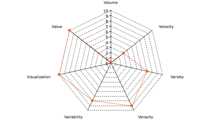
Chart by amcharts.com

Volume
Importance	1
Definition	The amount of data in question.
Data modeling relevance	Volume relates to the physical data model, which should be designed to take advantage of the data store. Volume is mostly a technology issue (i.e. data storage efficiency).

Velocity
Importance	3
Definition	The speed of data ingestion, as well as speed of delivering solutions to business problems.
Data modeling relevance	The ingestion speed is mostly related to the physical data model; it is mostly a technology issue (i.e. data store efficiency). Speed is also important for timely delivery of business solutions, which is why velocity scores 3.

Variety
Importance	7
Definition	The many different types of representations of data.
Data modeling relevance	Variety concerns representational issues, which should not affect the business facing side. This is mostly a technology issue (i.e. data preparation), but also a concern for the data modeler.

Veracity
Importance	9
Definition	The integrity, accuracy, and relevance of data.
Data modeling relevance	The three dimensions of veracity are meaning, structure, and content. Content veracity is mostly related to data quality, which is outside of scope here. From a modeling perspective, meaning and structure are of extremely high importance.

Variability
Importance	10
Definition	Brian Hopkins, Principal Analyst at Forrester, in a blogpost (http://bit.ly/29X0csP) on May 13, 2011, defined variability as “the variability of meaning in natural language and how to use Big Data technology to solve them.” He was thinking about technology like IBM’s Watson for easing the interpretation of meaning in the data at hand.
Data modeling relevance	Variability of meaning is a show-stopper. It should be handled properly. In the Big Data space machine learning is being applied. Read more about this in subsequent chapters.

Visualization
Importance	10
Definition	Graphical visualization of structure as an effective way of communicating complex contexts. This applies to both data visualization as well as visualization of metadata (data model in our context).
Data modeling relevance	Visualization of meaning and structure is the critical path to delivering real business value. You may develop a technically correct solution, but if your business users do not understand it, you will be left behind.

Value
Importance	10
Definition	You must get a working and meaningful solution across to the business, just in time. In addition to value, there is also the question of relevance. How do I, as a human, determine whether information is relevant for me and what the implications are?
Data modeling relevance	Business value is the ultimate goal of any project.

Michael Bowers1 has mapped the key issues of value and relevancy as shown here:

“Relevance for me” is subjective. As we try to make sense of a dataset, we look for a narrative that holds meaning for us. This narrative combines contextual information and relationships between elements into a body of meaningful knowledge.

Clearly, relevance and meaning are closely related. That puts relationships at the heart of understanding meaning.

Before 2000, databases were always described in some sort of schema. They contained names, data types, constraints, and sometimes also relationships. Many NoSQL technologies changed that.

“Schema on read” is a Big Data / NoSQL pitch that does carry some relevance. Schema on read refers to the ability to interpret data “on the fly.” Based on the structures (such as aggregates or document layout) found in the incoming data, a schema-like representation can thus be built as data is collected. “Schema on read” is quite close to the physical database, and there is a need for another layer to do the semantics mapping. That layer was previously known as the logical data model and will continue to exist for many more years. One of the important take-aways of this book is that the logical data model is indispensable and the book offers guidance on how to go about specifying the logical level.

Quickly pinpointing the meaning and structure of data is more relevant than ever; more and more data will be available in analytical environments, where the data should speak for itself. However, this does not necessitate the creation of schema. In fact, it means that getting a thorough understanding of the business and potential value of the data is likely more important than having a detailed schema.

Dr. Barry Devlin, an information architecture veteran and originator of the term “Information Warehouse,” recommends replacing the traditional schema with a “Modern Meaning Model (M3),” which replaces metadata with Context Setting Information (CSI). Context is what information ingestion is all about.

Given all these observations, one of the essential questions of data modeling becomes: How can we gain a thorough understanding of data’s business context—without spending months on modeling and creating schemas? After all, agility is key when it comes to delivering business solutions. This book will seek to answer this question.

2.3. Data Modeling Heritage

2.3.1. Evolution of Database

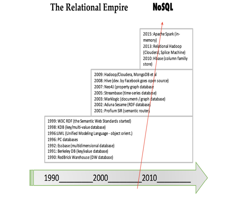
Before we understand where data is going, we first ought to be familiar with where it came from. Data modeling and databases evolved together, and their history dates back to the 1960’s.

The database evolution happened in four “waves”:

• The first wave consisted of network, hierarchical, inverted list, and (in the 1990’s) object-oriented DBMSs; it took place from roughly 1960 to 1999.
• The relational wave introduced all of the SQL products (and a few non-SQL) and went into production for real around 1990 and began to lose users around 2008.
• The decision support wave introduced Online Analytical Processing (OLAP) and specialized DBMSs around 1990, and is still in full force today.
• The NoSQL wave includes big data, graphs, and much more; it began in 2008.

Some of the game-changing events (in bold typeface below) and first-mover products (in normal typeface) are listed here:

Decade	Year	Event
1960’s	1960	IBM DBOMP (Database Organization and Maintenance Processor)
	1963	Charles Bachman Data Structure Diagram
	1964	GE IDS (Integrated Data Store)
	1966	CODASYL (Conference on Data Systems Languages) standard
	1968	IBM IMS (Information Management System)
1970’s	1970	Dr. E. F. Codd: A Relational Model of Data for Large Shared Data Banks
	1973	Cullinane IDMS (Integrated Database Management System)
	1974	IBM System R prototype, First version of Ingres
	1975	ANSI-SPARC 3-Schema Architecture
	1976	Peter Chen Entity Relationship modeling
	1979	Oracle
1980’s	1981	IDEF1 (ICAM Definition) - predecessor to IDEFX1 (US Air Force)
	1983	IBM DB2
	1984	Teradata (database appliance)
	1985	PC databases (for example dBASE, Clipper, FoxPro and many other)
	1986	Gemstone (object database)
	1988	Sybase, Microsoft, and Ashton-Tate port the Sybase relational DBMS to the OS/2 platform. Microsoft markets the new product as SQL Server and obtains exclusive rights on the Intel X86 platform
	1989	Kognitio (in memory database)
	The relational wave
1990’s	1990	RedBrick Warehouse (data warehouse database)
	1991	BerkeleyDB (key-value database)
	The decision support “wave”
	1992	Essbase (multidimensional database)
	1996	UML (Unified Modeling Language) - object orientation
	1998	KDB (key/multi-value database)
	1999	W3C RDF (Resource Description Framework - semantics standard)
2000’s	2001	Profium SIR (Semantic Information Router, RDF-based content management)
	2002	Aduna Sesame (RDF graph database)
	2003	MarkLogic (XML document and graph database)
	2005	Streambase (time-series database)
	2007	Neo4j (property graph database)
	The NoSQL wave
	2008	Hive and Cassandra (developed by Facebook) go open source
	2009	Hadoop/Cloudera, MongoDB, and others
2010’s	2010	HBase (column store, the Hadoop database)
	2013	Relational Hadoop (Cloudera and Splice Machine)
	2015	Apache Spark (in memory) and Apache Drill (schema-less SQL)

This table is based on many sources; the timeline represents the judgment of the author

The relational wave had some opponents:

• The (mainframe) DBMS vendors, who were late to join the SQL bandwagon, and were replaced by DB2 and Oracle
• The object-oriented DBMS, which never really gained a lot of territory
• Most recently, the NoSQL battlefield.

The data modeling scene has evolved in steps as well:

1. Bachman’s data structure diagrams
2. Chen’s entity-relationship modeling
3. Falkenberg’s and Nijssens’ object role modeling
4. A handful of variations on entity-attribute-relationship modeling styles
5. IDEFX1
6. UML and its class diagrams
7. Semantic networks and other graph approaches.

Today, boxes and “arrows” (crow’s feet and many other styles) prevail, and much of the sophistication of the advanced modeling techniques goes unused. But graphs are making headway into very large applications such as Google’s KnowledgeGraph.

We will take a look at most of the above, but before we get into that we present a little “phrasebook”. For those of you who were not around in the 1970’s and the 1980’s, here is a small glossary of pre-relational terms:

Term	Explanation
BOM	Bill of material. The structure used in describing the parts of a product and their relationships. A multi-level parent/child structure that breaks the product down into components, or shows “where-used” relationships between shared components.
Broken chain	A disrupted chain of pointers, typically caused by a power failure in the middle of a transaction.
Co-location	A physical optimization technique where pieces of data which have strong relationships and similar volatility. Still used today in document databases and in aggregate designs.
Conceptual model	The business-facing data model.
Disk address	What it says: Unit, disk, track, block, relative offset within the block.
Entity	A business-level object.
Field	A data item containing information about a property of a type of record. Today called a “column” or an “attribute.”
Hashing	Calculating a disk address based on a symbolic (business-level or “calculated”) key.
Hierarchical database	A database organized in blocks, containing a tree of records, organized from top to bottom and left to right. Parent/child, master/detail, header/detail, and similar terms were used.
Inverted list database	A database based on indexing structures, some of which completely engulfed the data. The ideas are re-used today in materialized views, column data stores, and other NoSQL constructs.
Key	A business-level field being used for random access by way of indexing or hashing.
Logical data model	The data model describing a specific solution, independent of the physical database choice.
Network database	A database organized as sets of records connected by pointers.
Object	Originally referred to a business object. Later it was referred mostly to designed, technical objects in software.
OLAP	Online Analytical Processing. Became synonymous with multidimensional processing (early 1990’s).
OLTP	Online Transaction Processing.
Physical data model	The data model to be implemented in a database of choice.
Pointer	A database “address” that points at another record in the database. Address was typically a logical page number and a page index, allowing for some level of reorganization on the physical disk tracks.
Random (direct) access	Accessing data based on either hashing a key, indexing a key, or using a pointer (as opposed to sequential access).
Record	A row in a table. There was no concept of Tables. Instead the term “Recordtype” was used, see below.
Record ID	A pointer to a specific record in the database.
Recordtype	The name of the collection of records describing Customers, for example. The same meaning is used today for “entity types”.
Relationship	Introduced by Chen - before him the closest thing was “set” (in the network databases) or logical database (in IBM’s hierarchical parlance).
Schema	A set of metadata describing the structure and content of a database.
Set	A collection of records, tied together by pointers (next, prior, and owner). A set had an owner and zero, one or more members (of another recordtype, typically).
Transaction	The same meaning as used today for ACID transactions (Atomic, Consistent, Isolated, Durable).

Let’s have a look at some of the compelling events and first movers.

2.3.2. Pointer Database (DBOMP)

One of the very first data stores was from IBM (in 1960). Its predecessor, which ran on magnetic tape, was called BOMP (Bill of Materials Processor). It was developed specifically for large manufacturers.

When BOMP was adapted for disk storage technology in 1960, its name changed to DBOMP (Database Organization and Maintenance Processor). DBOMP was one of the first disk-based data stores.

DBOMP was based on the concept of pointers: the exciting opportunity that came with the new technology of using rotating disks for data storage. However, developers soon strayed from raw disk addresses in favor of schemes with blocks of data and index-numbers. The blocks of data could then be moved around on the disk.

Here is a greatly simplified bill of materials structure (called a “tree”) of a bicycle:

To read and manipulate bills of materials, a user needed to:

• Go from a product to the items used in that product, commonly seen as the “product structure tree.” Wheel assemblies, for example, consist of spokes, tires, and rims.
• Go to an item’s parent, or “where used,” item. Front forks, for example, are parts of the bicycle.
• Advance to the next item in the structure; if the last thing you accessed was spokes, you’d advance to tires.
• Advance to the next item in the “where used” set of records. In the bill of materials above there is only one product; in reality, wheel assemblies could be used in mountain bikes, city bikes, electric bikes, and more.
• Return to the prior item (either within the structure or in the “where used” set of records). For example, if you just read seat, you’d return to gear assembly.
• Position yourself within the structure using a “PART-NUMBER” lookup, and from there you can choose to continue either downwards (exploring the bill-of-materials structure) or upwards (exploring the where used relationships).

As you can see, all of these actions rely on defined relationships, which at that time translated into pointers. Here is a simplified view of the basic DBOMP pointer structures:

Here is a more modern depiction of the data structure:

What you see here is called Property Graphs today, but we are looking at DBOMP in the 1960’s. BOM handling is essentially graph traversal, which is standard functionality in graph databases. In SQL databases, BOM handling requires recursive SQL; this is not a skill for the faint-hearted. Here is an example:

WITH BOM (LEVEL, MASTERITEM, ASSEMBLY, QUANTITY) AS

(SELECT 1, MASTERITEM.PARTNO, MASTERITEM.ASSEMBLY, MASTERITEM.QUANTITY

FROM PARTS MASTERITEM

WHERE MASTERITEM.PARTNO = ‘01’

UNION ALL

SELECT PARENT.LEVEL+1, CHILD.PARTNO, CHILD.ASSEMBLY, CHILD.QUANTITY

FROM BOM PARENT, PARTS CHILD

WHERE PARENT.ASSEMBLY = CHILD.PARTNO

AND PARENT.LEVEL < 2

)

SELECT PARTNO, LEVEL, ASSEMBLY, QUANTITY

FROM BOM;

The pointer-based disk addressing was used in later DBMS products, including IDMS and Total. Pointers at that time were largely physical; you risked serious data corruption in case of somebody pulling the power plug of the disk drive, for example. The pointer still lives on (in a more virtual manner) today in the many new graph DBMSs, which are part of the NoSQL wave.

2.3.3. Hierarchical Workhorses

IBM’s hierarchical database system IMS (Information Management System) and its little brother DL1 (Data Language 1) were for many years the workhorse DBMSs of many large corporations. From the 1970’s into the 1990’s, a case like a large bank with all its transactions was a serious performance challenge. IMS was considered the best bet, but it was rivaled by the network databases (compared below).

For an example, consider the idea of school courses:

• Each course has an instructor
• There may be 0, 1, or more students present at any given meeting session (or “instance”) of a course
• There is probably just one room assigned to the course, but the room may vary over time.

In a hierarchical database, the data store would be optimized for read access to all data related to any given course instance. This would be achieved by the concept of “physical co-location,” in which a database exists as a hierarchy of “segments.” Segments are retrieved by way of their root segment:

Based on information from IBM’s Knowledge Center online

These six named segments are stored sequentially according to their place in the hierarchy: top to bottom, left to right. The parent-child relationships are top-down; there can be zero, one, or many parent-child relationships.

A course with all its students, the instructor, reports, grade, and room information would be stored in one physical block. (Today, this would be called an aggregate.) Access could be physical sequential (from the first course in the database and onwards), index sequential (based on a symbolic key, e.g. Course Number), or direct (using a kind of hashing mechanism).

Sometimes the model would need to span hierarchies. One of the ways to achieve this was “logical relationships,” which spanned two hierarchies and appeared as new, logical hierarchies:

Based on information from IBM’s Knowledge Center online

In many cases, IMS did a very good job indeed. It took years before DB2 gained similar levels of performance. On the negative side, IMS had a very complex and inflexible architecture that turned relatively small changes into large re-engineering projects.

2.3.4. Programmer as Navigator

The 1973 Turing award lecture was given by Charles M. Bachman, the inventor of the first database system (1964). He described the new opportunities arising from the introduction of random access disk storage devices. The title of his talk was “The Programmer as Navigator.” Primary data keys were used as the principal identifiers of data records, but secondary data keys were also employed.

Besides records and keys, Bachman chose the metaphor of the simple set for relationships between records. Not sets in the strict mathematical (algebraic) sense, but like “collections”. To illustrate his point, Bachman presented a data model example with a department-employee set, consisting of sets of employees working in departments.

The physical model was based on “database keys,” which were close to physical pointers. Relationships (“sets”) would be navigated with forward (NEXT) as well as backward (PRIOR) and upward (OWNER) pointers, using the aforementioned database keys.

It’s here that the notion of the programmer as navigator originated. Sets were navigated in all directions throughout their hierarchical relationships. The paradigm was called the “network database” at that time.

Consider, for example, employees and departments. A department would be identified with a primary data key such as “department number.” Employees would be identified with another primary data key, say “employee number.” Beyond this simple identification, we might need to identify relationships; this is where secondary data keys would come into play. Bachman actually invented the first kind of entity-relationship modeling. He called it a data structure diagram. The version below was (and still is) used with the IDMS database system, which appeared in the 1970’s:

Bachman’s data structure diagram was the first of many “boxes and arrows” diagrams. Most of the text annotations in the diagram are physical specifications for IDMS. Notice, however, that the relationships (“sets”) are named.

The relationships were implemented as pointer-chains:

The pointers were present in a prefix to each record in the database, which was organized as pages with lines. Sets could be empty:

Or sets could have members as shown on the following page.

All of the links (called “sets”) in the diagram are implemented as pointer chains (next, prior, and owner being the options).

IDMS quickly became the main rival of IBM’s own hierarchical database management system (called DL1) and later the up-scale Information Management System (IMS).

The major drawback of IDMS was that of broken chains in case of a power failure. That meant manually repairing pointer chains...sometimes in the middle of the night.

The network database context was clearly algorithmic: procedural programming. From 1987 to 1998, the leading database periodical was called “Database Programming and Design.” The idea of programming was starting to gain traction, even in the context of databases.

2.3.5. Chen, Entities, Attributes and Relationships

The network database fit nicely with the entity-relationship data model that emerged around 1976. Peter Chen2 was the paradigm’s champion.

The diagram on the next page is a simplified Chen-style entity-relationship data model of our earlier departments-employees example.

Notice that in the original Chen style, the attributes are somewhat independent. The relationships between entities and attributes are visible. Later on, in the relational model, they were called functional dependencies. Also, the relationships between entities are named, and carry cardinalities.

There is no doubt that Chen wanted the diagrams to be business-facing (i.e. what was then known as “conceptual”).

In 1975 (one year before Chen published his paper), the ANSI-SPARC standards organization published its “3-Schema Architecture.” In this architecture were three levels of models:

• External views
• Conceptual models
• Physical models.

The ANSI-SPARC committee had great intentions, but what happened was really counterproductive. The “conceptual” disappeared from the business-facing level and became the “logical data model.” The data world filled up with tables and relationships and not much more. The conceptual and logical levels (if available) comprised high-level boxes and arrows. In the physical level, the addition of physical specifications (like indexes and tablespaces) necessitated the creation of physical models.

The rise of entity-relationship modeling took development in other directions. One such offshoot was IDEF1X from the US Air Force. Here is a sample IDEF1X-style diagram:

http://bit.ly/2ax3s01, by itl.nist.gov [Public domain], via Wikimedia Commons

The attributes were folded into the entities, which became tables. The diagrams began to fill with little icons, giving them a distinctly engineering flavor. At this point, conceptual models almost completely disappeared; most analyses started at the “logical” data model level. For instance, the following “logical data model” was inspired by a Microsoft MCSE training package from 2001:

See the original “Pubs” database diagram at http://bit.ly/2ax3KUB

With the advent of SQL, relationships were no longer named or shown. To this day, I’m not sure why relationships became second class citizens. From a business semantics point of view, this was a very sad loss of information.

2.3.6. Relational Model

In 1970, the “Relational Model” was published by Dr. Ted Codd3. The relational model started as mathematical theory. It evolved into a full-blown conceptual framework for what was perceived as a forward-looking data model. During the late 1970’s and much of the 1980’s, Dr. Codd toured the world giving seminars on his model.

Here are the key components of the relational model, some of which undoubtedly helped to usher in a huge paradigm shift:

• Programmers should not know the physical data model. (The relational model was intended to be a completely logical data model without notions like indexes, etc.)
• The tables are the key components.
• There should be no algorithms in database access—only the defined ways of set algebra (in the mathematical sense).
• The tables should be normalized, and intra-table relationships should be defined using primary and foreign keys.
• All keys should be business keys (no surrogate keys allowed).
• Integrity should be maintained by the DBMS.
• Database access should be handled by the DBMS (evolving the “query optimizer“ component).
• There should exist absolutely no pointers!
• The database structure should be able to change without affecting the programs (with regards to access paths).

The SQL language (Structured query Language) came out of IBM’s database research labs in the mid 1970’s. Before long, SQL was layered on top of several relational implementations.

This ultimately unhealthy marriage of SQL and relational models caused considerable confusion in terminology.

• A SQL table is not a relation (in the mathematical sense). Nor is it a relation variable (“relvar“), because relvars are predicates.
• A tuple is not a row in an SQL table, but a proposition.
• An attribute is not a column, but part of the heading of the tuple.
• SQL tables are not general-purpose abstractions to be used in all application areas.

The term “relvar” was introduced in 1995 by Chris Date and Hugh Darwen to create more precision in the discussion. The problem was (and remains) that “relation” refers to a construct of a named collection of attributes. In other words, it’s a metadata object. A given instance of a relation is a “variable” (or name) that implements that relation within a given set of data. The proposed abbreviation of “relvar” was too abstract for most people, and it never caught on. Instead the term “entity type” prevailed, although it is not part of the relational paradigm. It’s worth taking a new look at how relational data models can be designed. First, we’ll consider the general approach developed by Chris Date; he formed the methodology of “normalization,” which has been dominating the data modeling discussion for so many years.

The supplier-parts data model developed by Chris Date in his many books (e.g. [3]) has these three relvars:

The relvars are: S (supplier, upper-left table), P (parts, lower-left table) and SP (supplier/parts, the table to the right). In practice, “tables” are used much more often than “relvars,” and tables have “rows” and “columns.” However, “attributes” are also found in many textbooks.

In Chris Date‘s most recent book, he also uses the term “property.” In discussing the detection of where attributes belong in relvars, he proposes that STATUS moves to the SP relvar (as detailed below). But he then continues: “Intuitively the wrong place for it, since status is a property of suppliers, not shipments.”

Unfortunately, that opens up two new questions:

• If status is a property, why call it an attribute at all?
• From where is it concluded that status is related to suppliers? There are no indications of the dependency.

In Date‘s opinion, design theory is “largely about reducing redundancy.” Nevertheless, he quotes Dr. Ted Codd for saying “...task of capturing...more of…the meaning of data is a never-ending one…small successes can bring understanding and order into the field of database design.” I strongly agree with Dr. Ted Codd that capturing meaning is of utmost importance and that it leads to understanding and order.

The major lasting contribution of the relational model is the focus on functional dependencies, which lies at the very heart of data modeling. “Functional dependency” was originally a mathematical term indicating that something (a concept) is completely derived (by way of a function) from something that controls it (and possibly many other concepts). For example, a status attribute is describing something very specific, upon which it is “functionally dependent.”

Let us revisit the STATUS column of the Supplier relvar, S. Is it describing the status of the supplier or of the city? What if it is depending functionally on CITY? Here is S:

There is certainly some redundancy. We could eliminate it by splitting the Supplier relvar S into two, SNC and CT:

SNC (the table to the left) establishes the relationship between supplier (SNO) and city (CITY), whereas CT (the table to the right) establishes the dependency between city and status. No information is lost in the process. The relationship between CITY in the two relvars is called an “equality dependency;” in SNC, CITY is a foreign key, which references CT. STATUS has found its home as an attribute completely dependent on CITY.

“Third normal form” is defined as the desired state. It simply means that all attributes are functionally dependent on the primary key of the relvar. STATUS is directly and only dependent on CITY above. Still, it is important to remember that third normal form (3NF) is not necessarily the best normal form. Here is the relvar SNP in 3NF:

The relvar is in 3NF, but there are two sets of candidate keys: SNO+PNO and SNAME+PNO. QTY is functionally dependent on both of those keys. The remedy is to decompose (or “project”) the relvar into two:

SNAME was the trouble, but splitting the relvar into two solves the problem. The resulting model represents Boyce/Codd Normal Form (BCNF). Getting the keys and functional dependencies in order is the target of normalization.

Relational design also seeks to consider join dependencies. Date introduces the example of relvar SPJ:

The new attribute, JNO, stands for “job number,” and the relvar represents a ternary relationship. It consists of three keys and nothing else, so there are no problems with dependencies.

That relvar (SPJ) is in BCNF, and it can be decomposed into the three basic relvars:

The join dependency of the third table eliminates inaccurate content (the spurious line); hence the so-called join dependency (and the decomposed tables) are not redundant. Another point of critique for the normalization approach is that it is “backwards,” in that it starts with a body of data in an undefined state. Then it works its way through successive decomposition steps to arrive at the normalized relational data model.

Why this perspective? Well, it likely has much to do with the situation originally faced by data modelers:

• Forms on paper being manually entered into computers
• Sequential processing of punched cards or magnetic tape files
• Hierarchical data structures in IBM (and a few other’s) DBMS offerings
• Network data structures in pointer-based DBMSs.

Back then, conceptual structures were only in their infancy and did not provide much help to the morass of IT programs filled with incomprehensible, abbreviated, short data names (many with a maximum of 8 characters!).

Another significant impact of normalization came from the realm of development frameworks. User interface classes dictated the structure of supported data models. Deviations from a hierarchical super-table / sub-table structure were hard to work around.

A major achievement of the standardized, relational database world was that of improved usability. Programming-free, end-user access blossomed because of the simplicity of the relational model itself, and later because of the graphical user interfaces. The relational model is a nice fit for general purpose reporting tools, but graphical user interfaces quickly became what everybody wanted on top.

Finally, it is fair to say that physical requirements have had significant impact on the data models that run enterprises today. Great strides have been made in hardware and associated technology.

2.3.7. The Great Database War of the Eighties

Some argue that IBM prematurely commercialized its System R laboratory prototype into SQL/DS and then DB2. This is because Cullinet (IDMS), Software AG (Adabas), Applied Data Research (Datacom), and Cincom (TOTAL) had obtained high levels of account control in relation to the dwindling population of DL/1 and IMS accounts. Controlling the DBMS of a corporation was indeed an attractive position to be in.

However, Oracle was quick to build a commercial product, and within a few years, the migration from pre-relational to relational databases was unstoppable. A number of new vendors (like Ingres, Informix, and Digital) joined the bandwagon, but IBM got what it wanted. DB2 became the strategic DBMS for many large corporations. Around 1990, Oracle, Ingres, Informix, and DB2 matured into robust production DBMS offerings.

Thus database programming became focused on set algebra (except for stored procedures). No navigator was required—just a mathematician or logician. Tasks like recursive queries still posed challenges to algebra-focused programming, though. It took some 10 more years to really finesse; as recently as the early 2000’s, people were writing procedural-stored procedures in languages such as PL/SQL (Oracle) and Transact SQL (MS SQL Server).

People have criticized SQL for being unstructured and incompatible with queries, and for being an incomplete language (in the mathematical sense). Given its issues, the question arose: if getting SQL was the ultimate goal, was it really worth the effort?

From a price/performance point of view, IMS and its contenders (the inverted list systems DATACOM and ADABAS, and network databases TOTAL and IDMS) were unbeatable. Their weaknesses were flexibility; physical database changes were difficult to accomplish. Almost everybody used SQL as an interface around 1990.

But the “real SQL“ databases like DB2 and Oracle won out in the end. The replacement projects of legacy databases in IMS and IDMS started to take up too much of the IT department’s valuable time.

By the way: the algebraic correctness of the relational model has been challenged recently. Algebraix Data’s Professor Gary Sherman, supported by database veteran analyst Robin Bloor, claim that the structural problems dealt with in many of the classic relational examples are due to the fact that relational algebra is strictly not a proper algebra (because it is based on set theory, but it cannot be used on sets of sets). (See their free book The Algebra of Data, which can be downloaded from: http://www.algebraixdata.com/book.)

Evidently, people slowly began to realize that one size rarely fits all. Many modern products have SQL interfaces, but some do not need them. New and ingenious ways of handling data stores by using key-value pairs and columnar structures have changed the data landscape. Add “schema-less” to the equation, and you have some really nice flexibility.

This is what growing up is all about: learning by doing. After some trial and error, we now know that relational models aren’t enough.

2.3.8. Objects Galore!

A “resurgence” against the relational movement was attempted in the 1990’s. Graphical user interfaces rose in popularity, and they required advanced programming environments. Functionality (like inheritance, subtyping, and instantiation) helped programmers combat the complexities of highly interactive user dialogs.

“Object Orientation” proved to be just such an environment, and it quickly became widely popular. Another advancement came from the Unified Modeling Language, (UML). They developed a new style of diagram called the “UML class diagram,” as seen in this iteration of our department-employees example:

UML class diagrams focus on the logical level, and are declarative. But they are somewhat “stuck in the middle” between the business data model and the physical data model. The business data model should be business friendly; UML is not exactly that. Unfortunately, many so-called “conceptual models” (the model type name used for a product shown to the business people) are not intuitively easy to read.

And the physical model is still predominantly a relational, table-based model; normalized to the best extent that time permitted and budget allowed for, denormalized for performance, and only moderately digestible for business people. Object-to-relational mappings introduce additional complexity.

2.3.9. Graph Models

To make up for the deficiencies of UML class diagrams, graphs emerged as popular data models in the late 1990’s. The development took three paths:

• Semantic web standards
• Document referencing in document databases
• Pure directed graph technology.

Note that graphs were not new concepts, even at that time. Graph theory has been a part of mathematics since 1736! The first paper was written by Leonhard Euler and addressed the military problem of the Seven Bridges of Königsberg:

http://bit.ly/29VFWKh, by Bogdan Giuşcă (Public domain (PD), based on the image

Aiming to solve an optimization problem, Euler designed a network of four nodes and seven edges. The nodes represent the “land masses” at the ends of the bridges, whereas the edges (the relationships) represent the bridges. Working with that particular representation is called “graph traversal” today.

Today formal graphs are an established and well-researched part of mathematics. In the data modeling community, however, graphs emerged considerably later. The graph types of particular interest to data modelers are “directed graphs.” These are graphs where the relationships (called “edges”) between nodes are directed. Directed graphs are part of mathematical graph theory. That a graph is directed means that the edges have orientation (from one node to the other). The directions are typically shown as arrowheads on the connecting line visualizing the edge. Directed graphs are a good fit for semantics and, consequently, with data models (which represent business semantics).

One of the great misconceptions of the data modeling community has been that relational databases are about relationships. They are not. In fact, the relational model focused on “relations” (“relvars”) in the sense of having related attributes existing together, in the table representing a tangible or abstract entity (type). So the “relations” in the relational model are the functional dependencies between attributes and keys (which are also attributes). Traditional “relationships” (in the sense that there is a relationship between Customer and Order) are second-class citizens, labeled “constraints.” Some constraints are supported by “foreign keys,” which are as high as attributes can get (after primary keys, of course).

Consider the table relationships in the diagram above. Then consider writing the proper SQL joins for getting from A to Z. You wouldn’t be able to, would you? The semantics are unclear.

In a graph database, traversal is much simpler. Neo4j has an example on their homepage (http://bit.ly/29QHLq9) based on the Microsoft Northwind demo database (see diagram and property graph in section 5.1). The database is about products, orders, employees and customers.

Within the context of the referenced Neo4j example above a business question could be:

Which Employee had the Highest Cross-Selling Count of Chocolate and Which Other Product?

The graph could look somewhat like this:

Formulated in Neo4j’s query language, Cypher, the traversal looks like this:

MATCH (choc:Product {productName:’Chocolate’})<-[:PRODUCT]-(:Order)<-[:SOLD]-(employee),

   (employee)-[:SOLD]->(o2)-[:PRODUCT]->(other:Product)

RETURN employee.employeeID, other.productName, count(distinct o2) as count

ORDER BY count DESC

LIMIT 5;

(See more details at the Neo4j website referenced above.)

Notice how the path goes from product via order to employee to find the chocolate-selling employees, and then back via order to product to find those other products. “o2” is just a labeling of what we later want to count.

There are a number of good visual graph browsers available (e.g. Tom Sawyer, Linkurious, Keylines), with which you can perform traversals like the one above by pointing and clicking.

If you are dealing with highly connected data and want to be able to query it in many ways, consider a graph database solution.

Another interesting observation is that key-value stores and graph databases work quite well together. Nodes, relationships and properties are perfect candidates for key-value pairs. If the values relate to each other, you’ll achieve graph connectedness at minimal storage cost in physical configurations. High levels of transaction support (“ACID”) can be introduced, which has been the hallmark of relational DBMSs for decades.

The last ten years have seen the emergence of some quite successful commercial products. There are two primary paradigms, which are in use at more and more (and larger and larger) sites today:

• The “semantic web” category of graph databases, which involve networks of “triples” that represent subject-predicate-object “sentences”.
• Property graphs, which extend the directed graph paradigm with the concept of properties located on nodes, and also potentially on relationships.

One of the great challenges posed by the internet is matching data. The tough problems revolve around business semantics. This space is referred to as “The Semantic Web“ because much of the technology is based on standards developed by the World Wide Web Consortium (W3C)—the organization that also developed the specifications of HTTP, URIs, and the XML-family of standards.

Today the semantic web environment is based on the following standards, all of which are supported by robust technology:

• SKOS: Simple Knowledge Organization System. A system for management of vocabularies of concepts and relationships.
• OWL: Web Ontology Language. A system for management of ontologies (structured vocabularies based on logic) with inference possibilities.
• SPARQL: SPARQL Protocol and RDF Query Language. A query language for RDF databases.
• RDF and RDF Schema: Resource Description Framework. A definition and representation of concepts and relationships (the “data layer” of the semantic web).
• XML and XML Schema: Extensible Markup Language. This is the definitional platform for all of the above.

Precise definitions of the above are found at the website of the W3C consortium at www.w3c.org. All semantic web representations are expressed in XML. Schema facilities are available at different levels, but basic RDF data does not really require a strict schema in the classic sense.

OWL is by far the most feature-rich of the semantic web components. However, ontologies based on OWL are just as time-consuming to develop as UML (at a slightly lower level of complexity) and ORM/SBVR. However, OWL is very powerful; it performs well as a component of complex solutions with sophisticated requirements for the precision (quality) of search results.

SKOS is the “lightweight” component for the definition of controlled vocabularies. It is based on the notion of concepts and their relationships (quite similar to concept maps). We will focus on RDF in the following example.

Here are some facts about Woody Allen and some of his films:

• Woody Allen wrote To Rome With Love
• Woody Allen wrote Midnight in Paris
• Woody Allen wrote You Will Meet a Tall Dark Stranger
• Woody Allen wrote many more
• Woody Allen acted in To Rome With Love
• Woody Allen acted in Scoop
• Woody Allen acted in Anything Else
• Woody Allen acted in many more
• Woody Allen produced What’s Up, Tiger Lilly?

Consider RDF to be the “data layer” of the semantic web. RDF is based on the notion of triples, as illustrated below:

RDF “Graph” (simplified) of Movies related to Woody Allen

Each triple consists of a “subject,” a “predicate,” and an “object.” For example, take the triple Woody Allen (subject) wrote (predicate) Midnight in Paris (object). Each triple may be read as a simple sentence.

RDF may be stored in specialized databases, of which there are plenty (“RDF stores,” “Graph databases,” and more), or RDF may be provided as an interface to a database (either as part of a database product or as a “bridge” to a database product). SPARQL is the query language (quite technical) that comes with RDF.

The property graph model is a relatively late newcomer to RDF, based on these concepts:

Property graphs are essentially directed graphs consisting of nodes and edges (called “relationships” in the property graph context). In addition, property graph nodes may have:

• Properties
• Labels (typically used to denote the “type” of the object represented by the node).

Properties are used for storing data about the things that the nodes represent (called “attributes” in other modeling paradigms). Labels are provided for just that—labeling—in some systems (e.g. Neo4j). You would use “labels” to denote that one particular node represents a customer, whereas another node might represent a product.

Relationships are basically connections, but they can also carry names and other properties. Properties of relationships are recommended to be properties of the relationship itself, such as weights, distances, strengths, or time intervals. An example could be ownership percentages between some property owners, and the properties of which they individually own some parts.

There are a variety of property graph vendors. One of the most widely used products is Neo4j, which uses this example to explain the various possibilities for building representations of real-world situations:

Source: http://bit.ly/2ax29Ow

The property graph data model is a simple, powerful, general-purpose data model. For those reasons, I recommend using it as a generic representation of any data model. As you will see later on, it is easy to map from a property graph to any of the popular data models used in the SQL and NoSQL communities of the world.

2.3.10. Object Role Model (ORM) and Fact Modeling

In his seminal work, “The Entity-Relationship Model - Toward a Unified View of Data,” Peter Chen goes to the “binary level” before constructing his entity-relationship paradigm from bottom-level drawings, as follows:

What you see above is a directed graph representing a piece of a data model at the most “atomic level.” Chen’s work really is quite similar to the graph models depicted in the preceding chapter.

This level of detail is used by a school of modelers working with “fact modeling.” Their approach is not new, and was best known for many years as object role-modeling (ORM). It was supported by the popular Visio diagramming tool at the time that Microsoft bought the company behind Visio [7].

ORM is definitely at the right level of detail for data modelers (concepts and their relationships), but it also has all of the logic details required for formal, precise specifications.

I like ORM for many reasons. It is certainly more precise and detailed than the concept mapping discussed later in the book. ORM can handle even the most complex semantic challenges, and is adequate for describing business rules in general. However, precision comes at a cost. This makes ORM as complex as UML; consequently, it is not suited for business-facing specifications (the visual syntax looks too complex for most business people). Here is a very simple example of what today is called “fact modeling”4:

http://bit.ly/2adndNS By Jakob Voss (own work) [Public domain], via Wikimedia Commons

Today, modelers of business rules use fact modeling. It serves as the platform for the new business rule standard called SBVR (Semantics Of Business Vocabulary And Business Rules). This standard came out in 2008, and the Object Management Group (OMG) defines its scope as such: “This specification defines the vocabulary and rules for documenting the semantics of business vocabularies, business facts, and business rules” (OMG 2008). Business rules are outside of the scope of this book. As a resource, I recommend the Business Rules Community: www.brcommunity.com. You will find there many knowledgeable people working at the very difficult issue of business rules automation.

Another observation is that the complexity of ORM is on par with UML class diagrams, and also with the semantic web OWL standard. That makes sense, because fact modeling (ORM) is for business rules engines, UML is for object oriented programming, and OWL is for inference engines.

2.3.11. New Keys in the Models

One of the assumptions in the simple variety of relational modeling is that primary keys (and by definition then also foreign keys) are single-valued. In many cases, though, this is not the case. Concatenated, complex keys are common on the business level.

Furthermore, even single-valued business-level primary keys can cause problems:

• Primary key values (e.g. employee number) may be reused by the business after a few years, causing trouble in historical data.
• Consolidation of data from different sources may lead to key clashes.
• The same physical object instance (e.g. department) may change its key (department number) for any number of reasons (e.g. organizational changes).

The notion of the “surrogate key” evolved to address those issues. Keys were first mentioned in the article “Relations and Entities”5 in 1976. The idea is that the business level key is mapped to a system-generated, unique, surrogate key (typically a complete non-information-bearing number). This is considered by many the best practice in relational design today. There are also some terminology issues here. “Key” is not part of the business terminology, except for a few specific business subject areas. “Primary” and “foreign” are not familiar in the business context, either. What happens is that terms like “ID,” “identifier,” and good old “number” are used instead.

As for the uniqueness aspects, data modelers have adapted the very appropriate term “alternate key,” typically denoting the business-level (singe- or multi-valued) key(s). The term is internal to the model and is not business-facing.

So what you end up is typically something like:

• A physical primary key as a surrogate key (with uniqueness controlled by DBMS-level features)
• A business-level “identification”
• A business-level “name”
• The business-level (alternate) key fields with support from a DBMS-level features.

Let us look at a subset of the department-employee example in this context:

The system-maintained physical primary keys are called “ID” in this example. This is common, although I prefer the suffix “key.” The business level “identifications” are EmployeeNumber, DepartmentNumber, and ProjectNumber. The absence of business-level identifications on the “many-to-many” entity types is questionable. It could be argued that introducing, for example, a “Project Work Registration No.” would clarify matters.

2.3.12. Data Modeling Conclusions

If we summarize the data model progress in terms of the Turing Awards related to data modeling, we get this picture:

• 1973: Charles Bachman with “The Programmer as Navigator”
• 1981: E. F. (Ted) Codd with “Relational Database: A Practical Foundation for Productivity”
• 2001: Ole-Johan Dahl and Kristen Nygaard for ideas fundamental to the emergence of object-oriented programming
• 2014: Michael Stonebraker with “The Land Sharkx are on the Squawk Box.”

In hindsight, it is observed that data modeling was invented “on the fly.” The results were diverse and sometimes counter-productive to one another. Now, however, pragmatism has come to the rescue; there seems to be a great opportunity to solidify the best methods of modeling data.

Let us look back at the history of database in a slightly different manner, as shown on the facing page.

There was a lot of ground to cover for the pioneers of Database Management Systems, and they have done a fine job. The first twenty to twenty-five years introduced and fine-tuned important technological fundamentals such as:

• Physical disk space administration
• Pointers
• Records
• Indexes
• “Random access” schemes (later called “hashing”)
• Physical data model schemes based on hashing
• Physical co-location of data having similar volatility or life-cycles
• Multi-user concurrent update
• ACID (Atomicity, Consistency, Isolation, Durability) principles of transaction integrity and consistency
• Two-phase commit
• Journaling, logging, and recovery
• Memory caching
• Fault tolerance
• Distributed systems
• DBMS hardware.

The relational proponents were struggling in the 1980’s, with two major issues:

• Complexity of data modeling (“normalization …”) and of SQL
• Performance.

Even in its heyday, there were quite a few analysts who were not 100% sold on the omnipotence of the relational model. Yes, there were some good intentions and some good ideas. However, even to this day some serious criticisms of the relational model persist:

• Recently a mathematical incompleteness claim has come from a company called Algebraix Data. They claim that the relational model as defined by Dr. Codd is not really a consistent model since it cannot support sets of sets.
• Other criticisms accused SQL of not being a “well-formed” and complete (in the mathematical sense) computer language.

What really turned relational DBMSs into reliable, performant, scalable production tools was the advent of robust query optimizers. In 1979, Patricia Selinger of the IBM research center in San Jose described the optimizer of the IBM System R (a relational prototype system). Optimizer technologies matured during the 1980’s and established the “relational empire” around 1990, as shown on the facing page.

I have chosen 1990 as the start of the “relational empire” because by then, the cost-based query optimizers had reached sufficient sophistication to allow the RDBMS products to take over most of the database processing across most industries.

Not much new relational technology was published through the 1990’s and early 2000’s. In fact, entrepreneurs (in California, mostly) were busy developing alternatives to the relational approach. Quite a few of the new companies and products were focused on specialized niches such as documents, graphs, semantics, and high-volume applications.

Today, vendors unite under the NoSQL / Big Data brand. In one white paper, a non-relational vendor (MarkLogic) very succinctly complained of relational models: “Relational database vendors are still offering users a 1990’s-era product using code written in the 1980’s, designed to solve the data problems of the 1970’s, with an idea that came around in the 1960’s.”

Around 2008, triggered by Facebook’s open source versions of Hive and Cassandra, the NoSQL counter-revolution started. This space gets all of the attention today.

2008 was indeed a turning point. This can also be seen in the report of the very influential summit of database researchers, which have met in 1989, 1990, 1995, 1996, 1998, 2003, 2008 and 2013. In 2008, big data was the number one factor for a “sense of change” (The Claremont Report on Database Research, downloaded from http://bit.ly/2abBidh on 2016-02-27.)

So, where do we go now? How to balance the “what” and the “how” in light of NoSQL and all of the new technologies?

Well, the modern development platforms use schema-free or semi-structured approaches (also under the umbrella of NoSQL). “Model as you go” is a common theme, while data modelers and data governors are seen as relics from the past. Surveys (e.g. Insights into Modeling NoSQL, A Dataversity Report 2015, by Dr. Vladimir Bacvanski and Charles Roe) confirm this. Modeling for NoSQL is very often performed by the developer on the fly.

Database veteran David McGoveran notes this important distinction: the IT programmer’s perspective is that of rapid solution delivery, whereas the data modeler’s perspective is that of working with a long term asset (http://bit.ly/29PpWIJ).

How then can we choose what to carry over from the data modeling legacy, if anything at all? That is what the remainder of this book is about.

We will look at:

• The real business requirements for a data modeling solution
• A good architecture for a modern approach
• How to get the whole thing going.

Before we can really understand any of that, though, we must understand the nature of our clients, employers, and readers: other human beings.

2.4. Perception, Cognition and Psychology

2.4.1. Perception and Cognition

“Know your audience” has always been sound advice for communicators. As data analysts, our audience is primarily business-facing; even developers need to understand the business-level concepts. To deliver value to businesses, we must first understand how business people perceive and work with recognized information. For a better understanding of this, we turn to the realm of cognitive science.

Cognitive psychology comprises areas of research such as:

• Categorization
• Knowledge representation
• Language
• Memory
• Perception
• Thinking.

I have been wondering for several years why we, the data modelers and system architects, create drawings resembling engineering blueprints when we try to communicate to our business-level clients? Try showing a UML class diagram to a C-level executive. Talk about communication breakdown.

To help analysts and business clients speak a common language, we can turn to cognitive science. A number of paradigms have been proven by research to work effectively for better communication.

Concepts matter

Psychologists who specialize in learning and teaching have developed a technique called “concept mapping,” which is used in both elementary and higher levels of education with very good results. Concept maps are visual structures, which are easy to communicate. Consequently, they are a good platform for sharing user stories, which help us determine the requirements of the business.

Cognition is spatial

There are strong indications that our perception and recall capabilities are derived from our innate ability to visually process our environment. In other words, spatial structures are what matter most to our brains. On one side, this pushes analysts in the direction of visualization. On the other, it suggests we work with multidimensional coordinates. You’ll often hear the term “conceptual spaces” tossed around in this regard.

Semantics are important

Since approximately 2000, technologists (also called semantic web nerds) have worked with implementing semantic technologies. At the time of this writing, the field is blossoming with brand names that run their businesses on top of semantic technologies. If in doubt, read up on Google Knowledge Graph, and try it out for yourself.

Cognitive computing is here

Knowledge graphs and even more integrated solutions are now readily available from Silicon Valley and elsewhere. Check out a company called Saffron (saffrontech.com), and you will see what I mean.

Let me re-emphasize visualization. It is really a powerful thing. Visual perception works on approximations, which makes sense from an evolutionary standpoint; if you were in the jungle and noticed something that might be a tiger, well, might was good enough for you to run. In this way, our perceptive systems have been strengthened by millions of years of evolution and now work quite well—even on erroneous input.

Rinadeg Oedrr

Aoccdrnig to a rscarhee at Cigdmabre Uinervtisy, it deosn t mtetar in waht oredr the ltteers in a wrod are, the olny iprmoatnt tihng is taht the fnst and lsat ltteer be at the rghit pclae. The rset can be a taotl mses and you can sit11 raed it wouthit porbelm. Tihs is bcuseae the huamn mnid deos not raed ervey lteter by istlef, but the wrod as a wlohe.”

The example above6 highlights the way that memory supports the quick scanning of words in a document—not all letters are needed to derive meaning. Our brain can fill in the blanks on its own.

This brings us to the multidimensional aspect of data. The success of the multidimensional data model in business intelligence and analytics is overwhelming. Thinking dimensionally seems to come quite naturally to us.

This is probably because dimensional thinking is very similar to spatial cognition. At the “junction” of several dimensions, you find the information you need. So, multidimensional solutions give natural answers to the key question of location: “Where is this?” In fact, a “location” in a context is nothing more than multidimensional coordinates. Spatial thinking is again working wonders.

Recent research indicates that the hippocampi organs in the brain play a crucial role in providing access to the navigable representation of the both sensory experiences and conceptual constructs. The hippocampi are two finger-sized structures in the center of the brain (here in cross-section):

CC-BY-SA-3.0 (http://creativecommons.org/licenses/by-sa/3.0/), via Wikimedia Commons

The cortex layers of the brain consist of billions of neurons. Our memory creation (and hence recognition) functions are based on reinstatement of paths between locations; the locations themselves are targets of different perceptions created by senses and reinstatement. Memories that last longer than, say, half a minute, strengthen connections between the relevant parts of the cortex and your hippocampi. Since the hippocampi have connections in many places, they are thought to play the role of the integrator. Having an IT mindset, this reminds me of some sort of a “hyper index.”

Powerful communication can be achieved using the brain’s physical senses. We rely on visual information for about 80% of our situational perception; clearly, using visualization in communication is a must. Brains are built, not least, for navigation. That is why structured representations in 3-dimensional space are generally the most effective visual tools.

This book presents an approach to data modeling based on these cognitive findings. Is it possible to do data modeling without tables and schemas? You bet. And it might just work more effectively, too.

2.4.2. Concept Maps

Concept mapping comes from the field of learning psychology, and has proven to be useful to both business experts and business analysts (Moon, Hoffman, Novak, Canas, 2011, [11], and Frisendal, 2013 [5]). Concept mapping involves intuitive, visual communication. While conceptual modeling (UML and entity-relationship diagrams) failed as business-side tools, concept mapping is readily accepted in its place.

Concept mapping traditionally deals with people, language, and meaning—not engineering. The issue of becoming familiar with what a business is currently doing and where it wants to go is a people-based issue. It involves brainstorming workshops, mapping the language of the business, and getting the meanings right. A business may not even have a good grasp on their current situation; concept mapping can help them figure out their starting point and ultimate goals.

Contrary to common wisdom, business analysis is not “just a documentation issue.” It is a learning process both for the analyst and for the business itself. Concept mapping works in this context because it is based on psychology (the theory of meaningful learning), not on an engineering mindset.

Let us examine a simple example: The EU-Rent Car Rental.

The EU-Rent Car Rental is a fictitious business used in the OMG documentation for the Semantics for Business Rules and Vocabulary standard, SBVR, (http://bit.ly/2abzjp7).

The EU-Rent case study was developed by Model Systems, Ltd., along with several other organizations of the Business Rules Group (www.businessrulegroup.com), and has been used by many organizations. The body of descriptions and examples may be freely used, providing its source is clearly acknowledged.

The user story goes as follows:

EU-Rent rents cars to its customers. Customers may be individuals or companies. Different models of cars are offered, organized into groups. All cars in a group are charged at the same rate. A car may be rented by a booking made in advance or by a ‘walk-in’ customer on the day of rental. A rental booking specifies the car group required, the start and end dates/times of the rental and the EU-Rent branch from which the rental is to start. Optionally, the reservation may specify a one-way rental (in which the car is returned to a branch different from the pick-up branch) and may request a specific car model within the required group.

EU-Rent has a loyalty club. Customers who join accumulate points that they can use to pay for rentals. EU-Rent from time to time offers discounts and free upgrades, subject to conditions.

EU-Rent records ‘bad experiences’ with customers (such as unauthorized late return from rental, or damage to car during rental) and may refuse subsequent rental reservations from such customers.

The text above is pretty clear and well written. However, experience has shown that representing the same information in a concept map will make it more intuitive to read and understand. The diagram below represents almost all of the information in the text above:

The concept map really speaks for itself, which is the whole idea. Notice that you can read little sentences like “customer issues booking” and “car group has a rate” just by following the flow of the map. Full sentences don’t actually exist, but our brain has enough information to “fill in the blanks” thanks to the connecting lines between the concepts. Concept maps can be drawn easily in brainstorming workshops; they are easy to maintain and accessible for non-technical users.

Another key benefit to concept maps is that they rarely represent one-way narratives with a “start” and a “stop.” Mapping a concept reveals a sort of “lifecycle” for the user’s story.

You start by getting an overview of the whole story. The model on the facing page captures an overview of our car rental business.

From there, you must break down the objects shown on the overview, adding more detailed information. You may also “roll up” concepts and properties from forms and database descriptions, from the bottom up. You could, for example, look at a booking form and transfer the fields found on that to the concept map. Doing this adds more detail and in practice you work in a combination of top-down and bottom-up, depending on which information is available.

Here is a map of the information breakdown of the cars object:

Here is a short description of the syntax used in detailed concept mapping:

Round icons symbolize business objects, which can include physical objects (e.g. goods), documents (e.g. invoices), players / agents (e.g. people, organizations), or events/transactions (e.g. sales, posting, distribution).

Square icons with rounded corners symbolize the characteristics (or properties) of business objects, (e.g. product weight).

Square icons with sharp corners are used occasionally to exemplify one or more values of a property (e.g. “British Racing Green” or “Red”). This is purely for pedagogical reasons.

Connecting lines indicate relationships between concepts. If the connection is made with an arrowhead, it indicates a one-to-many relationship (e.g. multiple passengers per trip). Without the arrowhead, the meaning is that there is either a 1-1 or a 0-1 relationship. Either type of line may also indicate that there is not a relationship. For example, there may be a situation where a new customer has not yet bought anything. These variations are expressed by using modifiers like “has” or “may” within the text of the relationship.

The approach described above has been refined since its introduction in 2005, thanks to the support of a number of clients in both private and public sectors. No IT or data modeling background is necessary for the participants in the process. Business stakeholders get a strong and real sense of ownership of the business information asset. Concept mapping is intuitively easy to use and is ideally suited for brainstorming sessions around a data projector.

However, this particular method of concept mapping is just one communication method. Feel free to create your own style. What matters is that the concept maps communicate meaning well to business people. Remember to work from the top down and from the left to the right when creating and then explaining a diagram.

In addition to the concept maps, many analysts also capture and record (in Word or Excel) information about:

1. The verbal definitions of the concepts.
2. The necessary long-term business rules.

Verbal descriptions could be along these lines: “Concept: Car Movement. Definition: Planned movement of a rental car of a specified car group from a sending branch to a receiving branch.”

Sometimes people mistake “mind maps” for concept maps. There are two major differences between a concept map and a mind map:

• The concept map is organized top-down (and possibly also left-to-right). The mind map has emphasis on a central concept in the middle of a hierarchical structure. Concept maps are directed graphs with restrictions on structure.
• In the concept map, there are concepts (in the boxes) and “linking phrases” (the named relationships between concepts). Most mind maps do not name the relationships in this way.

Concept maps were originally designed and developed by Professor Joseph Novak (Novak 1990, 2008) with a learning focus. The theory behind concept maps is based on Professor D. Ausubel’s work on meaningful learning. This theory of meaningful learning suggests that learning is based on representational and combinatorial processes, which occur only when we receive information.

In other words, there are two processes: Discovery (of information) that leads to reception of the information (a.k.a. learning), integrated with what the learner already knows. In this manner, concept mapping is not only facilitating learning, but also creativity.

The key to successful concept mapping in the business setting, then, is to clearly depict the relationships between the basic concepts and terms used. Learning then takes place by assimilating new concepts into existing conceptual structures known to the learner. That is precisely what Professor Novak designed concept maps to do (Novak 2008).

The psychological aspects of concept mapping relate closely to those cognitive processes that help analysts better understand their clients and users. This is why I highly recommend using them for business-facing concept models. This is an area with some standardization:

• The International Institute of Business Analysis (IIBA) recently released Business Analysis Body of Knowledge (BABOK) version 3, which devotes a new section to concept models.
• A solid standard exists for concept models: OMG‘s Semantics of Business Vocabulary and Business Rules (SBVR).

Sometimes working with concept maps creates new insights (or “aha moments”). My book on business concept mapping [5] uses this concept map to outline the ideas of the book:

We won’t get into much more detail about the analysis process, so I’ll refer you to that book to learn more. It will be helpful if you are facing major analysis and design work having large and/or complex user stories.

The tool that I use for drawing the concept maps is called CmapTools. It is based on theoretical work done in the eighties and the nineties by Professor Joseph D. Novak. The tool as we know it today was developed around 2000; it picked up speed in the educational sector a couple of years later. Today, the publisher of the software is the Florida Institute of Human and Machine Cognition, IHMC.

The tool, which is free, can be downloaded from its website at http://cmap.ihmc.us. It is intuitively easy to use and is ideally suited for brainstorming sessions around a data projector. There are plenty of sources of guidance to CmapTools on the Internet, not least on IHMC‘s website: http://bit.ly/2aaZlI5.

2.4.3. Conceptual Spaces

We humans have strived to understand the structure of meaning for as long as speech has existed. Since data models essentially “speak” to their readers, we must consider the way we humans actually interpret meaning.

Advances in both neuroscience and cognitive science still point in many directions (because there are many issues), but there is a clear convergence toward a field called “Cognitive Spaces” (see, for example, The Geometry of Meaning - Semantics based on Conceptual Spaces, [6]).

A “meaning domain” consists of a set of values, which are points in a space; the space is structured according to categories, qualities, or dimensions. Think of spaces as a mathematical coordinate system (in reality with many more axes):

http://bit.ly/2b3eqKl. I, Sakurambo [GFDL (http://bit.ly/1fd019p), CC-BY-SA-3.0 (http://bit.ly/K9eh9h) eller CC BY-SA 2.5-2.0-1.0 (http://bit.ly/1pRlnje)], via Wikimedia Commons

In this manner, there is a geometrical distance between objects; this is a more precise representation than the brute force “similarity” measured by machine learning algorithms, for example.

Note that there may exist both perceived qualities, which we handle psychologically (sensory data of color perception, for example), and abstract qualities subject to cultural variations.

Gärdenfors uses an example of skin colors within the complete spindle of colors used by visual designers. I created a simplified representation of a skin color subset of a conceptual space:

Objects come in categories, which are frequently related in quasi-hierarchical ways. At the bottom levels, we find that individual objects have coordinates placing them in the right, bottom-level subcategory relevant to the object.

Adjectives (properties) are certainly part of the picture. Categories (quality dimensions, according to Gärdenfors) also cover actions and events, meaning that verbs fit into the conceptual space, too.

These matters are important for making decisions about how to best represent data models. A network of directed objects (semantic graphs) is certainly a very intuitive way to represent semantic structures. Other technology paradigms (like the semantic web tools RDF and OWL) are quite powerful. However, they are not really semantic in the sense that cognitive scientists define semantics (as described above).

The field of conceptual spaces is certainly an important research area that strengthens concept-based modeling. Although conceptual spaces have evolved in academia over the last fifteen years, they still reside primarily there. However, they are increasingly being used in practice. There even exists an XML dialect called Conceptual Space Markup Language.

2.4.4. Knowledge Graphs

Google has introduced its new generation of web searching, called “knowledge graphs.” These knowledge graphs deal with meaning. According to Google, “The words you use in formulating your search can often have more than one meaning. With the knowledge graph we can understand the difference, and help you narrow your results to find just the answers you’re looking for.” (See http://bit.ly/2bg5C5s.)

Here is an incarnation of the knowledge graph that appears if you search for people, companies, or many other types of entities:

When you examine knowledge graph technology in more detail, you discover that a “knowledge graph” is essentially the same kind of structure as a concept map—just supplemented with technical details. Here I have sketched a little concept map of the knowledge graph items that we found in our web search above:

In the concept map above, I mixed both instances and metadata. This will help give you a picture of what knowledge graphs will look like in reality, from a pure metadata perspective. A knowledge graph is really a semantic network. Many semantic networks are based on the W3C (w3c.org) Semantic Web stack of tools:

The basic data level can be illustrated with graphs. Here’s an example of the level of RDF, in the style used by the W3C:

Source of the example: Semantic Web for the Working Ontologist, Dean Allemang, Jim Hendler, Morgan Kaufmann, 2011, also downloadable from the web: http://bit.ly/29Poshz

The diagram above is visualizing eight “triples,” all in the form of sentences (for example, “Shakespeare wrote Macbeth”); the triples can be combined into the semantic network. The metadata level for RDF is called the “RDF Schema,” and uses concepts such as types, properties, and sub-properties. So, England would be a country and King Lear a play. Working with structures like that, people (called “ontologists” when working in this field) or software (by way of text analysis) can set up precise definitions of semantics.

Note that “semantic web” standards (and the related “topic maps” standards) are being used heavily in “knowledge engineering” environments. Information science is crowded with people defining and using ontologies: technology-supported vocabularies that support complex logic to the level of being able to infer conclusions about complex scenarios. The logic implemented is very similar to that used in UML class diagrams. You can learn much more about Google’s knowledge graph and those of its competitors...just Google it!

2.4.5. Cognitive Computing Example: Saffron

Semantics is not restricted to search contexts. There is a company currently working to combine semantics with:

• Modern cognitive computing (the successor of Artificial Intelligence)
• Raw computing power
• Graph technology.

The company is Saffron Technology. I attended a presentation by Saffron at the SmartData Conference in 2015. They are active in some public sectors, and their main case in the presentation was from the healthcare realm: a recommendation system of coverage.

The environment Saffron created is very dynamic, incorporating “instant learning.” It is based on schema-free semantic graphs and non-parametric statistics. “Memories” are maintained by way of semantic connections in the graph, combined with statistical counts and conditional context. Much of the power of the reasoning (e.g. for building recommendations) is based on the concept of “similarity.” What is the cognitive “distance,” for example, to a similar item in the past? What was this item? What was done in that case, and with what outcome?

Saffron summarizes their big idea as being where natural intelligence (implemented as software) meets machine learning. Natural intelligence tries to mimic what we believe goes on inside our brains. We can assume that association is taking place, and some sort of contextual reasoning takes advantage of that. The learning process is autonomous. The newer technology of machine learning (also called “deep learning”) is a brute force (hardware and software) approach that is driven by large amounts of data coming from multiple sources. The algorithms employed are frequently proprietary, and are based on statistics, non-linear approaches, semantics, “neural networks,” and many more concepts.

Machine learning is in the big data space. It’s no longer hidden by artificial intelligence researchers in universities or born-digital companies like Amazon, Google, and Netflix. More importantly, it generates significant business value. Visit McKinsey for an example: http://bit.ly/1GLaOF4.

In summary, keep in mind two key points. First, remember that modern cognitive computing is based on increased understanding of neuroscience, of the structures involved in our perception and cognition, and of the most powerful computer of them all: the human brain. Second, understand that these technologies will continue to impact many areas of computing in the future (including data modeling, as you will see).

2.4.6. Ubiquitous Pointer

Pointing is a very basic gesture for humans.

http://bit.ly/29PoVjS by Hillebrand Steve, U.S. Fish and Wildlife Service [Public domain], via Wikimedia Commons

Nobody is in doubt about what the intention is, regardless of culture, language, or circumstance.

This is supported by sound science. Here is an abstract for an article in Developmental Review, Volume 30, Issue 4, December 2010, Pages 352–366, Authors: Cristina Colonnesia, Geert Jan J.M. Stamsa, Irene Kostera, Marc J. Noomb.

The use of the pointing gesture is one of the first ways to communicate with the world. This gesture emerges before the second year of life and it is assumed to be the first form of intentional communication. This meta-analysis examined the concurrent and longitudinal relation between pointing and the emergence of language. Twenty-five studies were included into the meta-analysis, including 734 children. The role of several moderators was examined: pointing modality, pointing motive, age at which the pointing was measured, the assessment method of the pointing gesture and language development, the modality of language, socioeconomic status, and country. … It is concluded that the pointing gesture is a key joint-attention behavior involved in the acquisition of language.

It’s no coincidence, then, that objects called “pointers” have appeared in (and disappeared from) different data models for decades. (See chapter 2.)

Ted Codd, the inventor of the relational model, spent a lot of energy arguing against having pointers in databases. Admittedly, some of the physical implementations of pointers in Codd’s time had some serious drawbacks. Collectively known as “the broken chain,” pointers often pointed at the wrong places due to physical mishaps (like a power outage during an update of a chain of pointers).

Regardless of Codd’s skepticism, pointers are here to stay. Today they proliferate corporate databases under the disguise of “surrogate keys.” Nowadays, of course, the physical implementations are a lot better and more robust, backed up by indexes and key / value storage schemes. Tripping on a power cord isn’t such a devastating experience.

The pointer is one of the strongest visualization tools in our possession. That’s why I heavily favor directed graphs, such as concept maps.

2.4.7. Think Spatially

As detailed in the previous sections in this chapter, there seems to be serious value in leveraging concepts and conceptual spaces. Think spatially. Think in terms of locations and proximity. Think in context.

Here is an example of a person (John. F. Kennedy) and his personality profile (as per IBM Watson, based on JFK’s inauguration speech):

Source: http://bit.ly/1wXMi4D

Each of the axes in the diagram above represents a coordinate (for example Intellect 98%). Together those coordinates describe a location in the space, where the person is to be found; which describes the personality. The more dimensions you know (that is, the more context that you have), the more precisely you can determine what is in the location pointed to by the collection of dimensions. This is what both concept mapping and conceptual spaces are all about. The spatial metaphor is a very strong way to describe how the brain works under the perceptive process leading to cognition. You – intuitively – get the feeling “I know what this is about”, which actually means that you have navigated the conceptual space (neural network) and located something in there. If you know it beforehand (“been there, done that”), the realization comes to you. If you “have not been there before”, you might get fascinated about something new and potentially interesting; you might decide to “go there” to find out more.

What matters most is that the dimensions are clearly defined in an easily recognizable language, which the observers understand intuitively. That language, in the context of this book, is the data model as it is expressing itself towards the people who need to understand it.

Visualization has been a recognized need in data modeling for many years, but the particular style used matters more than one might think. The concept mapping style is a proven way of effective communication and is incorporated in our way of presenting data models.

Finally, pointing is another way of addressing something. If pointers were not effective, you would likely not use a computer mouse or a touch screen—both of these gestures are, in essence, ways of pointing.

The natural conclusion, then, is that visual representations of structure should be based on pointing (i.e. with arrows). This takes us back to concept maps, which from a mathematical perspective, are essentially directed graphs. Arrows undoubtedly support meaningful learning. When you develop a data model, you are an educator—always remember that!

The five guiding principles of modern visual communication of structure and content are:

Now that we understand how to best communicate with our readers, we can more closely consider our data modeling options.