Chapter 3 Real Requirements of Data Modeling

Data modeling is about exploration and discovery. We go to unexplored (or under-explored) territories and try to elicit meaningful knowledge from the clues we find there. We are always looking for relationships and patterns, which convey the structure of the landscape that we tour. We then write our findings as maps for others to profit from, should they desire or need to follow in our footprints.

So, using this expedition metaphor, let us begin by asking some basic questions:

• Why should we do data modeling in the post-relational world while on our expedition?
• What are the observations of other travelers that have been there before us?
• Which skills and tools should the cartographer use when mapping the new territory?

3.1. Post-relational Data Modeling

Traditionally, data modeling has followed a process like this:

See Scott Ambler’s good overview at: http://bit.ly/XALNgy

The first three activities are the classic processes associated with modeling. The next two (dotted) processes are quite useful, and are the hallmarks of good craftsmanship. The final three steps bring the modeler closer to the physical model. Conceptual modeling has faded away in favor of the “Great Pragmatic and Quick Unified Data Modeling Practice.” Even in the legacy relational systems development universe, agility has moved up on the list of priorities, leaving conceptual modeling “on the bench.”

If you zoom out a little, you see that the “unified” process is trying to accomplish two aspects of developing a good solution:

• Describing the “what” (in terms of a conceptual / logical data model)
• Describing some aspects of the “how” (e.g. physical access optimization via denormalization for better performance).

To truly understand this unified process, we first must get better at distinguishing between the “what” and the “how.” In other words, we must understand that the conceptual-level model has a place independent of the solution-level and physical-level models. Second, we must realize that the logical data model is an artifact designed by people, not something given beforehand. It encompasses design decisions about scope, generalizations, abstractions, and aggregations. Finally, we must understand that the physical data model has a whole lot more emphasis in the NoSQL world than in the relational world.

Given the variety of data stores and mirrored physical data models, we need a layer on top of them—one which is business-facing and still detailed. This is the role of the logical representation. It should remain unchanged regardless of the physical implementation. Despite their independence, developers need a firm grasp of both; they must first understand the logical model in order to implement it physically.

Business users need to be presented with the logical model whenever they access the data in the system. Today, all kinds of data are targets for analytics; as such, they are not always protected by a home-made application containing rules and mappings to the business terminology.

This matches the best practice of using “user stories” for business / user level requirements. Deconstructing the user story is a conceptual-to-logical modeling process. The actual construction of the solution data model results in the logical data model layer in the middle. Underneath that follows (in a later process) the physical layer. This 3-layer architecture embraces user needs and terminology on one end, and the necessary physical data aspects on the other. The focus of this book is the logical data model, which really is a solution data model.

Ever since “sort/merge” was invented with the magnetic tape revolution in the 1950’s, the need for data models has been evident. (For those of you who never worked with tape-based computing, understand that we actually built hierarchical data models on tape using “record type” fields to control the structure.)

In data modeling what we are looking for is meaning and structure. The whole purpose of the data model is to communicate the business meaning and the structure of the information, which describes the business contents of the database.

Meaning is really owned and defined by the business in question. They have the privilege of deciding on their own terminology, setting their own goals, and ultimately telling their own story. To effectively communicate these business stories, we first need to nail down the business semantics. There are a few different ways to accomplish this.

Structure is often defined by somebody else. When you describe a product, you have to describe physical aspects as well as some business aspects (price, maybe). If we are not talking about natural objects or events (such as animals, raw materials, the flow of water in a river, etc.), the objects are also designed by people. Understanding the structure is obviously necessary in order to grasp the significance and the context.

3.2. Finding Meaning and Structure

3.2.1. Working with Business People

Data modeling has been around for many years, but it’s still a work in progress. We have learned, after all, that one size does not fit all.

The growing realization is that relational DBMSs have their limits, and that other paradigms serve some circumstances better. Some of these circumstances in which DBMS might fail could be extremely high volumes (in which case key-values or Hadoop would better serve us) or highly complex data structures (in which case knowledge graphs and networks would be appropriate).

This realization gives us an opportunity to re-think how we support the data modeling process with all manner of thoughtful and productive data modeling practices. Wherever possible, we should strive to employ data modeling paradigms that work in different contexts and that provide an evolutionary path from the business level to the physical level.

But where to begin? Since these are business ventures, it’s prudent to start by defining the stakeholders.

The well-known “RACI” matrix (as defined in the IIBA Business Analysis Book of Knowledge, http://www.iiba.org/babok-guide.aspx) describes the roles of those involved in business analysis activities. It describes stakeholders as having one or more of the following responsibilities for a given task or deliverable:

• [R]esponsible: does the work
• [A]ccountable: is the decision maker (only one stakeholder!)
• [C]onsulted: must be consulted for input
• [I]nformed: will be notified of the outcome.

Each of these categories has the potential to include many stakeholders:

That is all well and fine, but the classic business analysis workflows are challenged because of rapid changes in:

• Requirement elicitation as user stories (not as formal specs)
• Project work styles (including iterative)
• New technologies, data stores, etc.
• Data governance “as you go”
• Data-driven analytics and big data.

The people, who are actively soliciting information (the producers of metadata and business process knowledge) are:

• business analysts
• subject matter experts
• data modelers
• developers.

The people contributing by way of consultation (sometimes called “the readers”) are either business specialists (i.e. subject matter experts) or the system owner(s), plus various kinds of architects.

I honestly believe that the subject matter experts should be given a key role to play; the more we can hand over to them in terms of producing a user’s stories, the better solutions we’ll be able to create in the end.

As you can see from the RACI figure, the data model has a lot of “readers.” Consequently, it must be communicated across many competencies and priorities. For that reason alone, it makes a lot of sense to profit from a data model, which is as intuitively understandable as possible.

So, how do we “consult” those who know what we would like to know?

This process is one of extracting user stories. It is akin to exploration, and must be supported by way of easy, intuitive, and efficient visualizations.

3.2.2. Concept Models as Part of User Stories

Working with concept maps to extract user stories is a creative process. In my book from 2012 [5], I combine it with design principles to create a process with three areas of focus:

Further explained in Frisendal, T.: Design Thinking Business Analysis - Business Concept Mapping Applied, Thomas Frisendal, © Springer, 2012

Begin by exploring the subject area using rough concept maps. These are visual user stories, if you will. Then take the most promising of those stories and develop them into prototypes by adding detail. Finally, choose the solution that seems most promising and finish it up by adding details about all relationships and properties. This may require two to four workshops, each lasting a few hours. Be prepared to map the concepts on the fly using a data projector and CmapTools, or a similar product.

The resulting concept map is ready for transformation into a solution data model, as will be explained in the next chapter. Here are some questions and guidelines to get you thinking about how to transform your concept map into a working solution:

Where to look? Where is the knowledge about the business? Obviously there are a lot of potential sources:

• Inside peoples’ minds
• In the business documents
• Inside operational documents such as charts of accounts, spreadsheets, IT data models and databases, and business intelligence reports.

Top-down or bottom-up? Doing a top-down deconstruction of the desired feature or information content is probably the most common pattern in designing user stories. However, it happens that you are driven by (legacy) data, in which case a re-engineering of the physical data model into a more business-friendly representation (concept model) is appropriate. You choose what is best. Sometimes a combination of the two works out fine.

Get the business pains out in the daylight! As you brainstorm your concept models in the preparation of user stories, you (and the business folks) do have some learning experiences. Expect some surprises. Here are some frequent discoveries:

• Our terminology is imprecise or arcane, perhaps born out of tradition
• Some of our concepts are plain wrong
• “Is this really what we are doing?”

and other such “aha moments.”

Generalization is your friend. Frequently you run into challenges in handling complex contexts. By tradition, maybe, some business concepts have evolved into a “spaghetti” of too many concepts and relationships; not always in a coherent structure. It is indeed best practice to strive for simplicity. And your weapon in this situation is to generalize the structure that you see into a simpler structure using less but more general concepts. This is something you should always have in the back of your head. “Can we find a simple representation of this that provides the same or better business value?”

Start simple. Use circles for all concepts in the beginning, when you are brainstorming or sketching a map.

Identify relationships. Very clearly name all the relations between concepts. Make sure everyone is on the same page about the terminology used.

• One-to-one relationships. Use a connecting line without an arrowhead to denote a one-to-one relationship between concepts.
• One-to-many relationships. Use a connecting line with an arrowhead at the “many” side to denote a one-to-many relation between two business objects.
• Many-to-many relationships. Carefully check whether there really is no business object in the middle of a many-to-many relation. If it is truly missing, use a connecting line with an arrowhead in each end.

Objects and properties. In later stages of the modeling flow, circles represent “business objects“ (or entity types). Rounded rectangles represent properties (or attributes, in classic data modeling) of objects.

Sample data. You may, at times, use squared rectangles to denote actual values (of data) for pedagogical purposes. Not all readers know all the concepts. So, in an attempt to explain, you could add some real data in the concept model. In section 2.4.2, you see “Fuel type” explained by visualizing some sample data like “Gasoline”, “Electricity” and “LPG”.

When to stop? Somewhere there is a border between the data model and business rules. Business rules tend to include specific data, whereas data models don’t. So, if you find that you are including data in the diagrams, do not do it, except for pedagogical reasons, maybe. Detailed rules should exist as textual descriptions, not as diagrams. Business rules should not reside within a data model, but may be kept in a separate document or a business rule elicitation tool.

Top-down page layout. Concept maps should be easy to read. Psychologists have shown that readers expect a top-down organization of the map.

These activities happen at this stage of the life-cycle:

Here is an example concept map from the world of shipping. It is a snapshot of a work in progress (the freight rates, for instance, still need to be elaborated):

Further examples can be found in Frisendal, T.: Design Thinking Business Analysis - Business Concept Mapping Applied, Thomas Frisendal, © Springer, 2012

“But wait! Could there be automated ways of doing this?” you should ask. What if we ask the data?

3.2.3. Functional Dependency Profiling

Saying “structure” is the same as saying “relationships.” Functional dependencies are relationships. As such, one would think that automated functional dependency checkers and explorers should compose a diverse and interesting set of tools.

Unfortunately, this is not the case. There are plenty of academic papers and projects on the topic, but on the commercial side, there is not a whole lot. Inside the big data modeling tools, you can find some.

In the early 2000’s, tools that actually look in depth at your data started to emerge. People realized that data always speaks for itself. Inside the data, you will find the truth about all the dependencies that are actually contained in them.

The products doing this are called “data profiling tools.” They are designed to catch all information about data by way of actually reading through them. A report containing the meta data is the result. Here is a definition from Wikipedia:

Data profiling is an analysis of the candidate data sources for a data warehouse to clarify the structure, content, relationships and derivation rules of the data. Profiling helps not only to understand anomalies and to assess data quality, but also to discover, register, and assess enterprise metadata. Thus the purpose of data profiling is both to validate metadata when it is available and to discover metadata when it is not.

https://en.wikipedia.org/wiki/Data_profiling

Data profiling software can be used to spot many things. In the context of data modeling we are very interested in learning more about:

• Potential inter-table relationships (also called foreign key relationships)
• Potential intra-table relationships (also called functional dependencies).

Let us suppose that we are looking at a database that contains “Product No” in one table and “Item No” in another table. It a good assumption that they refer to the same concept. We can ask that of the data profiling software by doing both inter- and intra-table matches of occurrences of the two sets of values. If Product No on the Orderlines matches Item No on the Items table, for example, there is some support for the assumption that we are looking at a (inter-table) relationship. The number of unmatched vs. the number of matched values determine the quality of the relationship. If, for example 95 % are match, it is very likely an intended relationship. But if the only 40% match the assumption has not been proven with any certainty. A classic Venn diagram can visualize this:

If the percentage of unmatched results is too high, the probability that you are looking at a significant real-life relationship is low.

This is quite useful. As a data warehouse modeler, I have been faced with the task of modeling a legacy system with highly undocumented physical data models (employing 12-character data names, and the like). Data profiling can provide help in understanding the data structures in the bowl of data that you are looking at.

Most of the profiling tools I have seen work from a “quality” measure; the strength of the relationship between two sets of keys in one, two, or more tables is set to 100%, if everything on one side matches the other side perfectly. What brings down the strength of the relationship is unmatched keys on either side. If the potential relationship is from A to B, it reduces the quality of the relationship. If there are values in B which are not matched in A, this could be a problem. That could mean Orderlines regarding unknown products. The other way around is more acceptable—it means unordered Products.

Consider another example, which is on the intra-table level: You are examining the result of a functional dependency check within a product table. It shows that there is a dependency between ProductSubCategoryID and Style. However, it has a quality of 95%, because there are violations. For one, the Style = “U” is found in four different ProductSubCategoryIDs; as such, the functional dependency does not hold completely. However, 95% match is a good starting point; somebody will have to clean up the 5% dirty data.

Most data profiling tools will indicate which rows support the relationship and which rows violate it.

If this had been the first time you visited that database, you would probably not know which level in the product hierarchy determined Style. After profiling the data, you not only know this, but you also know that there are data quality problems. One check with a data profiling tool has revealed a lot of useful information.

There are plenty of data profiling tools available in all varieties: open source, commercial, standalone, and as components of ETL and data integration products.

But can we do better? What about machine learning?

3.2.4. Mining the Semantics

There are even better technologies that can actively help you to distill the concepts and relationships in a given body of data.

Knowledge engineers and information scientists have for years employed tools for mining structured and unstructured data, in order to extract both data and metadata. Look for methods and tools within text analytics for things like:

• Data level:
  • (Named) entity extraction (data level, persons, companies, products)
  • Sentiment analysis
  • Text mining
• Metadata level:
  • Concept extraction / mining
  • Relationship, fact, and event recognition
  • Classification of documents.

Obviously, we as data modelers are mostly interested in extracting metadata in the form of concepts and relationships, which can be fed right into our data models.

Much of the above is document-centric, focusing on unstructured or semi-structured data. Frequently the word “modeling” is used more in the sense of data mining or statistical modeling than in the sense of data modeling. However, understanding the concepts and relationships is equally important whether you are a data scientist or a data modeler/developer.

Text analysis and analytics are heavy-duty technologies which incorporate sets of semantic/linguistic, statistical, and machine learning techniques.

In 2015, one of the information management old-timers, Informatica, released the “Live Data Map 1.0.” It is an impressive offering, which is positioned as a knowledge graph of all enterprise metadata, incorporating (among many other things) functionality for:

• Semantic Search with intelligent facets
• Related data assets
• Semantic content through data domains
• Business lineage
• Business glossary
• Relationship discovery.

These metadata points are continuously updated across the Informatica platform, for governance, data preparation, data extraction, and similar purposes.

At the end of the day, the most important function is relationship discovery. Understanding business semantics is closely related to understanding the structures of relationships, including dependencies. Discovery works by detecting the quality of cross-business object type relationships, as described above in the discussion of data profiling. There are two desired functionalities within relationship discovery:

• Automated suggestions of relationships (and accompanying keys)
• Visualization of relationships.

A new generation of data profiling vendors (including Paxata, Trifacta, and Tamr) are marching out in force these days as part of the big data and analytics space, with similar offerings based on semantics and machine learning. They are referred to as “data preparation vendors,” and they employ the same kinds of heavy-duty tools within areas such as:

• Data discovery
• Data transformation
• Data modeling / structuring
• Metadata catalogs.

They typically also offer workspaces, designed to be used interactively by business analysts (data scientists) using visual tools.

The Gartner Group has looked at these new data preparation vendors in some detail; they have compiled a “Market Guide for Self-Service Data Preparation for Analytics.”

If you let the data analysts do such machine-assisted data modeling without governance, you run a considerable risk of (A) getting more than one version of the truth, and/or (B) repeating modeling work that has already been done by somebody else.

You cannot model data in isolation from everything else. There is bound to be some overlap and you also need to integrate with other data in other systems or databases. You need to compare your data with other data, designed by somebody else in a different context and maybe some time ago. And this is what data models are for: learning from your new data model and comparing it with other models, discovered by other people.

Automate as much as you can, but have business people inside the loop in order to validate and consolidate the findings and the resulting data models. Visualization is a robust and quick way to achieve this validation.

3.3. Visualization of Models

3.3.1. Functional Dependency Visualization

One of the major contributions of Dr. Ted Codd’s relational model is the focus on the importance of functional dependencies. In fact, normalization is driven by a modeler’s desire for a relation where strict functional dependency applies across all the binary relations between the designated primary key and the fields depending on it.

As such, functional dependencies are very important contributors to the structural description of the information being modeled.

Inter-table dependencies are modeled as relationships; depending on the declarative language (e.g. SQL) they may be named (with a “constraint name”) or not.

Intra-table dependencies, on the other hand, are not present in the relational model. The only indication of their presence is the logical co-location in the table of the fields, which are guaranteed (by the data modeler) to be functionally dependent on the primary key and that alone. No arrows, no names, no nothing.

Since dependencies between data are key to creating a correct data model, we need to bring the dependencies out into the bright sun. They must be clearly explicated, like this pedagogical functional dependency graph on the facing page.

Unfortunately, not many people have worked with functional dependencies on the visual level as Bob Dewhurst does in the graph on the facing page.

In his seminal book “Introduction to Database Systems, Volume I” [2], C.J. Date creates little “FD diagrams” that show the relationships between attributes in relations. The attributes are each in small rectangles (similar to concept maps), but the relationships are not named.

Inspired by online learning pages from Charles Darwin University, Bob Dewhurst (http://bit.ly/29XOVvD)

Beyond functional dependencies, other spill-overs from normalization include avoiding redundancies and update anomalies. Date‘s famous supplier-parts example illustrates this:

This is in second normal form, which implies that it could contain redundancy (of city, for example). It also implies an update anomaly; it is impossible to register a city before you have a supplier in that city. City and Supplier are more independent than dependent. Supplier No (SNO) is not an identifying key for Cities. Yes, there is a relationship between Supplier and City, but having them in the same relation is not a good idea, because it hides important structural information (the relationship between supplier and city).

This relation is ill-defined because not all of its fields are functionally dependent on the same key. So, what the cookbook recipe of normalization is doing is identifying which relations (tables) are not well-formed (according to the mathematics behind the paradigm used by Dr. Ted Codd in his relational model).

Since the co-location is only on the visual level (in the data model), and since the physical model might be more granular than the tabular model (e.g. a graph database), normalization loses importance these days as a vehicle for eliminating physical redundancies and anomalies. However, normalization was also designed to help with identifying the inherent structures, and that remains a key obligation of the data modeler.

Detecting dependencies is still very important. One advantage of graph databases is that they make dependencies very visible. Here is a simple directed graph representation of the ill-formed relation above:

Visualization of functional dependencies is certainly a business requirement of data modeling. It’s a powerful tool for detecting dependencies and many more processes.

We have drawn diagrams over the last 40 years or more, but not all of them were highly communicative, as we have seen in chapter 2. The diagrams that we have been using, are actually drawn by engineers (data modelers) in order to be shown to other engineers (developers). That is all fine and well. In fact, UML and ER models work fine for programming tasks. But for business facing modeling tasks, they are too complex. We need simplicity. And we need visualization.

3.3.2. Understanding Structure and Content

If communication is our challenge, visualization is our solution.

To reflect a bit on the challenges that the relational model brought upon us, I will first turn your attention to the term “relation.”

What the term implies (loosely) is that the relation is a set of binary relations, and if all those relations are functionally dependent on the same function, the functional relation of all of the set members (or columns) is good to go. This relation will be stamped as properly normalized. Many people think “relationship” when they hear the term “relation.” And in terms of everyday semantics, that is perfectly right. For data modelers though, structure rules the world.

And structure is not handled well, at least visually in the classic relational model. Relationships are secondary citizens of relational. They are normally not named at all in the visualizations, and functional dependencies (i.e. the sources of meaning / semantics) are not visible or named. This goes for both inter-table and intra-table dependencies.

Our previous approaches to conceptual modeling, based on simplified entity-relationship diagrams or UML class diagram style visualizations did not communicate a lot of information to the business people. Normally they were very general and typically used for the one-page overview. The overview has its role, but it is not a business information structure diagram.

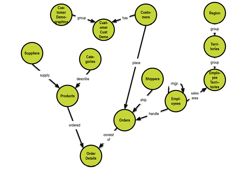
Concept maps, such as the example on the following page, communicate information structure extremely efficiently, and they’re easy to produce.

Notice the named relationships, which include the functional dependencies (for example, employee and salary), and notice how you can read the whole thing in short sentences. Imagine the same thing expressed as text. Surely, the concept map communicates clearly and quickly. But there is a drawback. While they’re more succinct than text-based user stories, though, they can still quickly become daunting in size. Can we find a more compact representation?

3.3.3. Property Graphs

We have looked at, what we can do to visualize structure. Let us now worry about content.

Given that structure is important, why then, do the classic data modeling practices all deliver content diagrams much like the model on the facing page, on the “logical” level?

The diagram above is filled with detail:

• Tables and their names
• All of the fields and their data types
• Primary keys and foreign keys (named by their constraint names)
• Relationships as “crow’s feet” with either dashed lines or full lines, signaling “mandatory” or “optional”.

The needed detail is present, but most of the space is used for listing table content (i.e. field lists).

Slightly simplified diagram built from the Microsoft Northwind documentation on the internet by the author using Oracle SQL Developer Data Modeler

Property graphs are directed graphs, just like concept maps, and they offer elegant visualization of structure, such as the example on the facing page.

If necessary, we can add the properties discretely like this:

Not all of the details about the data model are found in the diagram above, but we really do not need to have all details on all diagrams, always.

Properties of a business type are all at the same “location” by definition. It logically follows that the business object types are the “landmarks” of the data model. One size does not fit all. But property graphs come close to being the perfect candidates for a database-agnostic representation of data models.

Property graphs are similar to concept maps in that there is no normative style (e.g. like there is in UML). So feel free to find your own style. If you communicate well with your readers, you have accomplished the necessary.

3.3.4. Progressive Visualization of Data Models

Graphs are powerful, also on the data level. Here is an example from the Linked Data organization (http://linkeddata.org).

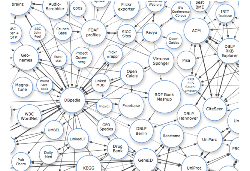
Part of a huge graph found on the Linked Data website; Creative Commons license

The linked data movement has been around for some years now, and it is still growing. Here are their own words about what they do:

Linked data is about using the Web to connect related data that wasn’t previously linked, or using the Web to lower the barriers to linking data currently linked using other methods. Specifically, Wikipedia defines “linked data” as “A term used to describe a recommended best practice for exposing, sharing, and connecting pieces of data, information, and knowledge on the Semantic Web using URIs and RDF.”

Source: http://linkeddata.org

In short, graphs represent complex relationships between data occurrences (nodes), in many different dimensions for all permutations, for which there are data. This is indeed, from a mathematical point of view, a large directed graph: a network of interconnected data. Also for data models, relationships play key roles in models (structure is what it is about!), and there is no better way to represent relationships than graphs.

So then, how do we turn our table models into graphs? Let us revisit with the Chris Date-style supplier/parts (SP) relvars, and transform them into a proper solution model in five easy steps. The relvars are called S (suppliers), P (parts), and SP (supplier/parts). Here they are, in tabular form:

STEP 1: Draw a naive concept map of S, P, and SP. (Note that this first map is just to get us started; no particular symbolism is needed in the representation yet.)

STEP 2: Visualize the relationships between S, P, and SP:

There is indeed a many-to-many relationship between S and P—only carrying the Qty as information. The foreign keys of supplier-part are S# and P#, because they are the identities of S and P, respectively.

STEP 3: Name the relationships:

Naming the relationships adds a new level of powerful information. Some relationships are rather vague (using the verb “has,” for example). Other relationships are much more business-specific (for example, “supplies.”) The data modeler must work with the business to find helpful, specific names for the relationships.

The presence of a verb in the relationship between supplier and city could well mean that it is not a straightforward property relationship. In fact, cities do not share identity with suppliers; suppliers are located in cities. (This is how to resolve functional dependencies.)

STEP 4: Resolving the functional dependency of city:

STEP 5: Reducing to a property graph data model, as shown on the next page.

Concepts, which are demonstrably the end nodes of (join) relationships between business objects, have been marked in bold. These were originally highlighted in the relationship name (“identified by”). This bold notation corresponds to C. J. Date‘s original syntax in his presentations, where the primary key columns had a double underscore under the attribute name.

All concepts in the preceding concept map, which have simple relationships (has, is...), and which only depend on the one and same referencing concept, have been reduced to properties.

3.3.5. Tool Support for Property Graphs

The plentitude of modern physical data model types means that there is no one way of visualizing them anymore. Some methods are indeed very specific.

One exception is in the semantics area, where there exist diagramming facilities for the XML-based standards used there.

Surprisingly, there are no “ivy league” data modeling tools available for using property graphs to represent data model designs. The graph DBMS vendors do have some graph browsing tools, but many of them are too generic for our purposes. On the other end of the spectrum, there are some quite sophisticated graph visualization tools available for doing graph-based data analysis.

I figure that the “ivy league” data modeling tool vendors simply have to catch up. While they are at it, why not go 3D? Who will be the first?

Fortunately, we are not completely without means.

3.3.5.1 White-boarding on Tablets

Several of the use cases for data modeling processes are in the explorative and ideation phases. In these situations, you need a lot of “white board” space. This may not be a physical white board, though. The modern tablets have good support for “assisted” white-boarding.

One of the successful products is Paper from Fifty Three (www.fiftythree.com). It runs on iPhones and iPads. You will probably find a stylus helpful for tablet white-boarding. Paper includes some bright assistance (originally called Think Kit), which is now included in the free product. (The stylus is not free, but alternatives do exist.) Your drawings look good, because the software corrects your sloppy drawing style. Check out the videos on the internet.

Paper can produce diagrams like this at the speed of thought:

3.3.5.2 Diagramming tools

The visual meta-models for property graphs as data modeling paradigms are rather simple and easy to set up using Omnigraffle or Visio.

Here is the style I used in Omnigraffle to make some of the diagrams used in this book:

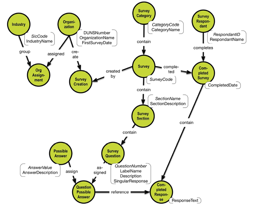
The example above (a survey form) is explained further in section 5.3. Omnigraffle is quite easy and does not require many clicks.

3.3.5.3 CmapTools

As previously discussed, I use the product CmapTools from IHMC for concept mapping. It is very easy to use, and you can draw as you go in a brainstorming session. You are not limited to the concept mapping style that I propose. The diagrams can be tweaked in many ways, and the tool is very productive.

Here is a little concept map style diagram drawn in CmapTools:

The diagram describes the structure of the property graph data model (simplified). CmapTools is available from this website http://cmap.ihmc.us. Please note that the basic IHMC CmapTools software is free for educational institutions and US Federal Government Agencies, and at this time the software is being offered free as a beta test version to other users, including commercial users.

3.3.5.4 Graph database browsers

The graph database products typically offer a browser as part of their user interface. Neo4j is one of the most popular graph databases in the NoSQL space (www.neo4j.com). A community edition is available for download. There are several ways of getting data into Neo4j. One way is to use a batch load from a CSV-file. You could collect the nodes (concepts) in an Excel sheet and load them into Neo4j using its Cypher query language. The Excel sheet should look like this:

The above node definitions are actually the nodes of the survey data model shown earlier in this chapter.

The load would be executed using a Cypher command like the following:

// Create BusinessObjects

LOAD CSV WITH HEADERS FROM “file:///SurveyMetadata.csv” AS row

CREATE (n:BusinessObject {ObjectID: row.ObjectID, Name: row.Name, ObjectType: row.ObjectType,

Property1: row.Property1,

Property2: row.Property2,

Property3: row.Property3,

Property4: row.Property4,

Property5: row.Property5,

Property6: row.Property6,

Property7: row.Property7,

Property8: row.Property8,

Property9: row.Property9,

Property10: row.Property10

})

One way of getting the edges (relationships) into Neo4j could be the following Cypher commands:

MATCH (a:BusinessObject), (b:BusinessObject) WHERE a.Name = ‘Industry’ and b.Name = ‘OrgAssignment’ CREATE (a)-[:group]->(b)

MATCH (a:BusinessObject), (b:BusinessObject) WHERE a.Name = ‘Organization’ and b.Name = ‘OrgAssignment’ CREATE (a)-[:assigned]->(b)

MATCH (a:BusinessObject), (b:BusinessObject) WHERE a.Name = ‘Organization’ and b.Name = ‘SurveyCreation’ CREATE (a)-[:create]->(b)

MATCH (a:BusinessObject), (b:BusinessObject) WHERE a.Name = ‘Survey’ and b.Name = ‘SurveyCreation’ CREATE (a)-[:createdby]->(b)

MATCH (a:BusinessObject), (b:BusinessObject) WHERE a.Name = ‘SurveyCategory’ and b.Name = ‘Survey’ CREATE (a)-[:contain]->(b)

MATCH (a:BusinessObject), (b:BusinessObject) WHERE a.Name = ‘Survey’ and b.Name = ‘SurveySection’ CREATE (a)-[:contain]->(b)

MATCH (a:BusinessObject), (b:BusinessObject) WHERE a.Name = ‘Survey’ and b.Name = ‘CompletedSurvey’ CREATE (a)-[:completed]->(b)

MATCH (a:BusinessObject), (b:BusinessObject) WHERE a.Name = ‘SurveyRespondent’ and b.Name = ‘CompletedSurvey’ CREATE (a)-[:completes]->(b)

MATCH (a:BusinessObject), (b:BusinessObject) WHERE a.Name = ‘QuestionPossibleAnswer’ and b.Name = ‘CompletedResponse’ CREATE (a)-[:reference]->(b)

MATCH (a:BusinessObject), (b:BusinessObject) WHERE a.Name = ‘CompletedSurvey’ and b.Name = ‘CompletedResponse’ CREATE (a)-[:assigned]->(b)

MATCH (a:BusinessObject), (b:BusinessObject) WHERE a.Name = ‘SurveyQuestion’ and b.Name = ‘QuestionPossibleAnswer’ CREATE (a)-[:group]->(b)

MATCH (a:BusinessObject), (b:BusinessObject) WHERE a.Name = ‘PossibleAnswer’ and b.Name = ‘QuestionPossibleAnswer’ CREATE (a)-[:group]->(b)

MATCH (a:BusinessObject), (b:BusinessObject) WHERE a.Name = ‘SurveySection’ and b.Name = ‘SurveyQuestion’ CREATE (a)-[:contain]->(b)

Having the property graph data model in the Neo4j graph store enables you to browse it using the standard browser in the base product:

The properties of the individual nodes are available below the graph, if you click one of the nodes to highlight it:

The browser is intended as a developer support tool, and it works for all your basic needs. You can modify the model inside Neo4j using the Cypher query language, which offers a full range of data manipulation functionalities.

There are several JavaScript libraries available for applying graph visualization on top of Neo4j.

3.3.5.5 Graph visualization tools

At the high end of capabilities (and yes, there typically is a license price) we find sophisticated graph visualization tools.

Of the most popular is Linkurious (https://linkurio.us). Their solution runs on top of Neo4j and other graph data stores.

Linkurious offers a JavaScript toolkit (linkurious.js) for building graph exploration applications yourself. But they also offer a sophisticated, out of the box solution (which comes with a commercial license).

The same property graph data model as shown above can be presented like this in Linkurious:

The graph is a bit compressed because of the little space available on a printed page in a book. The user interface on the screen is very usable indeed. Through the user interface you can add, modify, and delete nodes in your property graph data model:

You can also add, modify, and delete edges in your data model:

I am grateful to Linkurious SAS for their kind assistance in producing these screenshots.

The possibilities presented above are only a small subset of the features, functions, and vendors found in the graph visualization space.

Now we are ready to examine the “Requirements Specification” for data modeling.

3.4. Data Modeling Requirements

3.4.1. Solution Architecture

In my honest opinion we have not been particularly good at finding the proper levels of abstraction and specialization for the classic conceptual, logical and physical layers. But that does not imply that we should abandon a 3-layer architecture.

There is no doubt that on top we have a business-facing layer, which is based on knowledge elicitation by and from the business people. I prefer to call that the Business Concept Model layer.

The middle layer serves the purpose of containing the actual design of a solution to be implemented. It should ideally be subsetted from the business concept model and then extended with design decisions based on desired behaviors. I call that the Solution Data Model.

And finally, the good old Physical Data Model, as you would expect. The thing that is a transformation of the solution data model, and that a data store / DBMS can employ. This gives rise to this architecture of the Data Modeling system:

For a readable version of the illustration on the physical model level, see page 171.

As we begin to compile our list of data modeling requirements, this proposed layering of data models leads to these architecture level requirements:

Requirement 1: A three-level data model architecture.

Requirement 2: The business-facing level must be built on a concept model paradigm (for visualization and effective learning).

Requirement 3: The solution-level data model is independent of the data store platform, and is derived from the concept-level model.

Requirement 4: The physical-level data model is specific to the data store platform, but the content should be easily mapped back to the solution-level data model, by way of visualization (of, for instance, denormalization, collections, and aggregates).

Unfortunately, the physical modeling stage is beyond the scope of this book. Fortunately, there exist many other books that do a great job of addressing physical modeling aspects in their respective data store platforms.

3.4.2. Business Concept Model Requirements

The Business Concept Model is the business-facing side of the data model. This is pure business information, and is concerned with terminology and structure.

Requirement 5: The business level must support terminology and structure.

No system-related design decisions should be made here. But business level design decisions should be included as necessary.

Requirement 6: The business concept model should be intuitive and accessible for those stakeholders who know the business, but do not know the details of IT solutions.

Requirement 7: The terminology should be that of the business.

Requirement 8: The business concept model should be easy to produce and maintain.

A brainstorming work style is the typical elicitation process; there should be tool support for this task.

Requirement 9: There should be visualization tools available for concept modeling, and they should be easy for business people to use.

(Optional) Requirement 10: Automated elicitation procedures may be employed (such as text mining and machine learning).

Identity is not explicit, but uniqueness is implied by the references coming into the concept. This is because identity (more about that later) is frequently designed into the solution, whereas uniqueness is typically derived from a (combination of) business “keys.” The uniqueness criteria may be a bit vague on the business level, which warrants a designed solution for obtaining guaranteed unique identities (because that is what we can handle in IT solutions).

The following concepts should be supported:

Requirement 11: Business Objects.

Requirement 12: Properties of business objects.

Requirement 13: Atomic values (for illustration purposes).

Requirement 14: Named, directed relationships with simple cardinalities.

Requirement 15: A directed style for relationships between business objects.

Requirement 16: An undirected style for relationships between a business object and its properties.

Requirement 17: Generic data types (e.g., number, string, date, amount).

Requirement 18: Definitions of the terminology used (word lists with explanations and examples).

Requirement 19: Simple business rules written as text.

The Concept Model will consist of overview models and of detailed subject area-specific models, as necessary.

The scope of the model may define the scope of the solution, but that is its only direct relationship to the next layer.

Requirement 20: The Business Concept Models should be (at least) approved by the business people, including the sponsors.

Obviously, this spins off a whole lot of functional requirements, but a good concept mapping tool supplemented with Excel sheets and Word lists will do quite well.

3.4.3. Solution Data Model Requirements

What are the business reasons for creating a data model?

There are some categories of modelers:

• The Explorer: You are lucky; you develop a data model for a previously un-modeled subject area. No one in your organization has ever exploited this territory before. Wow!
• The Integrator: You are assigned the task of wrangling some data that was created by a system not developed by your organization, trying to whip the data into shape for integration with some of your own operational data. Good luck!
• The Data Scientist: You need to explore a lake of data, most of which is generated by exotic systems not homegrown in your own organization. May the force be with you!

These three modeling roles all share a strong requirement for being aligned with the business. This means talking the language of the business.

Maybe the Integrator is protected a bit, because they do not necessarily have to expose their solution data model. But they really need to understand the business terminology, and they must map the technical names of the implementation model to the business names of the solution model.

The general, high-level requirements of the solution data model can be expressed as follows:

We all need to communicate in the language of the business. Which translates into a need for doing a solution data model. Much of this book is about transforming data modeling from a rather technical and somewhat clerical discipline into a practice that is easy to perform, easy to understand and looks good. The focus should be on good craftsmanship. As you have seen already we have eliminated a lot of arcane complexity by simply going to a graph representation of the conceptual model, the concept maps. The solution data model continues the visualization strategy by using the property graph approach, as you will see below.

The Solution Data Model is created as a derived subset of the business concept model. After that, it is refined and amended.

Requirement 21: The solution data model is effectively derived from the business concept model.

This means that some concepts become logical business objects, whereas other concepts become properties of those business objects.

Requirement 22: The subset of the business concept model is gradually and iteratively extended with design decisions.

Requirement 23: It should be easy to establish the lineage from a design object to the business concept model.

The design decisions will typically enable specific, desired behaviors and solution oriented data.

Requirement 24: The solution model must be visual; the structures being visualized should resemble the structure of the business concept model.

This requirement actually follows from the derivation approach to solution modeling.

Requirement 25: Uniqueness constraints should be defined.

Requirement 26: Since identity is closely related to uniqueness, support for that should also be present.

Requirement 27: There should be support for identifiers, including surrogates.

Requirement 28: There will also be technical and auditing data specified as well as data designed to handle time aspects, such as time series data.

Requirement 29: Cardinalities will be defined on all relationships.

The following meta concepts should be supported:

Requirement 30: Business objects (concepts, which may be referenced from other concepts, and which have properties).

Requirement 31: Properties of business objects (properties are concepts, which share the identity of the business object that owns them).

Requirement 32: Named, directed relationships with precise cardinalities.

Requirement 33: Simple types (e.g. number, string, date, amount).

Today there are a number of physical models available, including:

• Graphs and triple stores
• Key-value stores
• Columnar and BigTable descendants
• Tables (like in relational and SQL methods).

The tabular (relational) model is just one of several. “Decomposition” of the tabular structures (the process known as normalization) is quite complex; it can end up being ambiguous if the semantics are not well defined.

On the other hand, mapping to a tabular result structure from other representations is rather easy—almost mechanical. This means that the tabular model is not a good starting point for a data model, but it might well be a good choice for an implementation model.

What is the good starting point, then? There are some contenders. On the conceptual level, people tend to fall into two camps:

• Those who prefer a business-facing, intuitively simple representation (as is the case with concept maps)
• Those who prefer absolutely tight control over semantics which can be found in various “modeling languages” such as:
  • OWL (the Web Ontology Language from the World Wide Web Consortium)
  • UML (Unified Modeling Language from the Object Management Group)
  • Concept Models are now part of the Object Management Groups (OMG) Semantics of Business Vocabulary and Business Rules (SBVR) standard; which is now adopted by the Institute for Business Analysis, IIBA, in their Business Analysis Body of Knowledge (BABOK) standard
  • ORM (Object Role Modeling supported by the ORM Foundation); a form of Fact Modeling.

Although different, these methods achieve very similar things, and they embed a palette of constructs in support of logic. Logic is necessary because much of computing is about predicate logic. However, logic makes things complex.

When it comes to logic, two of the most difficult decisions that must be made are:

• When to stop modeling data?
• When to start specifying business rules?

I am in favor of simple solutions. Of the four modeling languages mentioned above, the SBVR style concept models are comparable in simplicity to concept maps. Since I also want a data model solution level representation which is simple, communicative, and intuitive, I do not want to include business rules visualization at that level.

Concept maps, of which I am a great fan, are based on directed graphs. So are the semantic technology stacks (W3C’s RDF and so forth). Directed graphs seem to be a very good fit for communication structure. We will take advantage of that. The solution data model that we will work with in the remainder of this book is the Property Graph Model. It can look like this:

Requirement 34: Since directed graphs are behind most other data models as an inherent structure, the property graph data model is the chosen paradigm for representing solution data models.

It is important that the proposed relations between business objects be chosen such that they are (left to right) functionally complete and correct. This behavior was formerly known as normalization.

This concludes the requirements for the solution- (logical-) level data modeling process, and it prepares us for the transition to the physical data model.

3.4.4. On Using Property Graphs

What graph databases do very well is represent connected data. And as you have seen throughout this book, representing real-world is about communicating these two perspectives:

• Structure (connectedness)
• Meaning (definitions).

Together they explain the context very well. Nodes represent entity types, which I prefer to call types of business objects. Edges, better known as relationships, represent the connectedness and, because of their names, bring semantic clarity and context to the nodes. Concept maps exploit the experiences from educational psychology to speed up learning in the business analysis phase.

That is why the labeled property graph model is the best general-purpose data model paradigm that we have today. Expressed as a property graph, the metamodel of property graphs used for solution data modeling looks like the model on the following page.

The important things are the names and the structures (the nodes and the edges). The properties supplement the solution structure by way of adding content. Properties are basically just names, but they also can signify “identity” (the general idea of a key on the data model level). Identities are shown in italics (or some other stylization of your choice).

Physical uniqueness is essentially the combination of identities of the nodes included in the path leading to the node whose identity you are interested in. If uniqueness is not established in this intuitive way, you should consider remodeling or documenting the uniqueness in some special fashion. Business level uniqueness is controlled by composite business keys (marked in bold in the property list).

Data types may be added at this stage, but normally they only become important as you get into designing a physical data model. In the NoSQL area you have many more options, including packing things together into long strings or aggregates, as the situation dictates.

3.4.5. Physical Data Model Requirements

It should be easy to implement controlled data redundancy and indexing structures. The physical data model is, of course, dependent on the data store / DBMS of your choice.

Depending on the paradigm of the target system, you will have to make some necessary transformations. However, the solution data model is rather easy to transform into almost anything in a rather mechanical way.

Here are some examples of targets:

• Property graph
• RDF graph
• SQL table
• Key-values and column family store
• Document database.

Requirement 35: It should be relatively easy to establish the lineage from the physical model to the solution data model, and further on to the business concept model.

This is best done on top of the solution data model. In fact, in most cases it’s as easy as “lassoing” selected parts of the solution data model together, transforming them into aggregates, collections, tables, or any other abstractions necessary. More about that later. A denormalized structure could look like this:

The physical model will contain extensions to the solution data model in the form of performance oriented data, and structures for sorting, searching, and browsing in particular orders.

There will be physical constraints, such as unique indexes, as much as your data store permits. More about this later.

3.4.6. Keeping it Simple

In all that we do, we should try to keep things simple. What follows, then, is a complete list of the non-functional requirements for a robust contemporary data modeling “system,” as we identified above, for your convenience.

• General requirements
  • Requirement 1: A three level data model architecture.
  • Requirement 2: The business facing level must be built on the concept model paradigm (for visualization and effective learning).
  • Requirement 3: The solution level data model is independent of data store platform and is derived from the concept level model.
  • Requirement 4: The physical level data model is specific to data store platform but the content should be easily mapped back to the solution level data model by way of visualization of denormalization, collections and aggregates.
• Business level requirements
  • Requirement 5: The business level must support terminology and structure.
  • Requirement 6: The business concept model should be easy to understand intuitively by business people, who know the business, but do not know the details of IT solutions.
  • Requirement 7: The terminology should be that of the business.
  • Requirement 8: The business concept model should be easy to produce and maintain.
  • Requirement 9: There should be visualization tools available for concept modeling, and they should be easy to work with for business people.
  • (Optional) Requirement 10: Automated elicitation procedures may be employed (such as text mining and machine learning).
  • Requirement 11: Business Objects.
  • Requirement 12: Properties of business objects.
  • Requirement 13: Atomic values (for illustration purposes).
  • Requirement 14: Named, directed relationships with simple cardinalities.
  • Requirement 15: Directed style for relationships between business objects.
  • Requirement 16: Undirected style for relationships between a business object and its properties.
  • Requirement 17: Generic data types (e.g. number, string, date, amount).
  • Requirement 18: Definitions of the terminology used (word lists with explanations and examples).
  • Requirement 19: Simple business rules written as text.
  • Requirement 20: The Business Concept Models should be approved by the business people, including the sponsors.
• Solution level requirements
  • Requirement 21: The solution model is effectively derived from the business concept model.
  • Requirement 22: The subset of the business concept model is gradually (iteratively) extended with design decisions.
  • Requirement 23: It should be easy to establish the lineage from a design object to the business concept model.
  • Requirement 24: The solution model must be visual and the structures being visualized should resemble the structure of the business concept model.
  • Requirement 25: Uniqueness constraints should be defined.
  • Requirement 26: Since identity is closely related to uniqueness, support for that should also be present.
  • Requirement 27: There should be support for identifiers, including surrogates.
  • Requirement 28: There will also be technical and auditing data specified as well as data designed to handle time aspects, such as time series data.
  • Requirement 29: Cardinalities will be defined on all relationships.
  • Requirement 30: Business objects (concepts, which may be referenced from other concepts, and which have properties).
  • Requirement 31: Properties of business objects (properties are concepts, which share the identity of the business object that owns them).
  • Requirement 32: Named, directed relationships with precise cardinalities.
  • Requirement 33: Simple types (number, string, date, amount...).
  • Requirement 34: Since directed graphs are behind all other data models as the inherent structure, as well as for the business semantics, the property graph data model is the chosen paradigm for representing solution data models.
• Physical level requirement
  • Requirement 35: It should be relatively easy to establish the lineage from the physical model to the solution data model, and further on to the business concept model.

This is the result of trying to keep the list as concise as possible, while still scoping a solution that does the job with higher quality and speed than legacy approaches.