This chapter covers

• An introduction to graphs and graph terminology
• How graph databases help solve highly connected data problems
• The advantages of graph databases over relational databases
• Identifying problems that make good candidates for using a graph database

Modern applications are built on data--data that is ever increasing in both size and complexity. Even as the complexity of our data grows, so do our expectations of what insight our applications can derive from that data. If you are old enough, you likely remember when applications took a long time to load data and had limited features. Today’s reality is different; applications provide powerful, flexible, and immediate insight into data. But for every 100 questions modern applications answer, the most common data tool these use (namely, a relational database) handles only about 88 of those questions well. That leaves 12 types of questions where relational databases struggle. These remaining questions deal with the links and connections within the data, those aspects of the data that can generate powerful and unique insights. This puts us at a crossroad: we can use the relational database “hammer” to pound away at those questions and make this work well enough, or we can take a step back and look at what other tools can answer these questions better, faster, and with less effort.

By reading this book, you decided to take a step back from your relational database hammer and investigate a road less traveled: graph databases. This book is written for developers, engineers, and architects who are interested in other ways to solve problems specific to working with highly connected data. We assume you are already familiar with relational databases but are interested in learning when, where, and how graph databases are a better tool.

Our goal with this book is to equip you with the techniques needed to add graph databases as another tool in your toolbelt. We like to think of this book as the guide that we wish we had when we started building graph-backed applications. Throughout this book, we’ll demonstrate common graph patterns that highlight how graph databases enable navigation and exploration of data in ways not easily accomplished with a traditional relational database.

Our primary approach is through an example of building a fictitious restaurant review and recommendation application we call “DiningByFriends.” As we move through the software development life cycle from planning, to analysis, to design, and on to implementation, this application demonstrates how to think about and work with graph data. Each chapter builds on the previous chapter, and by the end of this book, we’ll have created a functioning application on a graph database. We believe that putting the concepts immediately to work by solving a realistic set of problems, even if they are somewhat simplistic, is the best way to get comfortable using a new technology. Let’s begin our journey with an introduction to what graphs and graph databases are and how they compare with traditional tools such as relational databases.

1.1 What is a graph?

When you look at a road map, examine an organizational chart, or use social networks such as Facebook, LinkedIn, or Twitter, you use a graph. Graphs are a nearly ubiquitous way to think about real-world scenarios as these abstract out the items and the relationships being represented, and this abstraction allows for quick and efficient processing of the connections within the data.

Let’s demonstrate with a common task: going to the supermarket. Take out a piece of paper and draw out a plan for getting from your house to your supermarket. Chances are it looks something like figure 1.1.

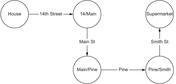
Figure 1.1 A graph representing directions to the supermarket

Figure 1.1 shows a graph where the key items and relationships are represented by abstractions. First, we abstracted key locations, like intersections, and represented these as circles. We then designated the connections between these key intersections as lines, showing how the key intersections are related. This is just one example of how we naturally represent real-world problems as graphs.

It is human nature to abstract real-world entities and their relationships, and the mathematical name for this abstract construct is a graph. When thinking about a set of data that contains a vast array of highly interconnected items, we might also describe this data set as a web of interconnected things, which is just another way of saying a graph.

On maps, cities are frequently represented by circles, and the roads that connect these are represented by lines. On an organizational chart (org chart), a circle usually represents a person, normally with an associated title, and lines that connect these people together show the employer-employee relationship. In a social network, people connect to one another via friending or following. This process of generalizing entities and the connections between them is the fundamental basis for graphs and graph theory. Because graphs have been defined and studied by mathematicians for centuries, we can offer these definitions used in graph theory as our starting terms:

• Graph --A set of vertices (singular, vertex) and edges

• Vertex --A point in a graph where zero or more edges meet, also referred to as a node or an entity

• Edge --A relationship between two vertices within a graph, sometimes called a relationship, link, or connection

While definitions are nice, graphs have the advantage of being simple to illustrate. When working with graphs, diagrams usually consist of circles representing vertices and lines representing edges, as figure 1.2 shows.

Figure 1.2 A graph is easily illustrated with circles for the vertices and lines for the edges.

Note We use the terms vertex and edge throughout this book. Some graph databases use the term node instead of vertex and relationship instead of edge, but these are conceptually the same.

Graphs are not new concepts to software developers. These are the basis of many common data structures that we use in software development all the time, likely without even realizing it. Common data structures such as linked lists and trees are simply types of graphs with specific rules applied to them. While these data structures are well known to developers, the actual implementation details specific to graphs are usually abstracted away.

1.1.1 What is a graph database?

A graph database is a data-storage engine that combines the basic graph structures of vertices and edges with a persistence technology and a traversal (query) language to create a database optimized for storage and fast retrieval of highly connected data. Unlike other database technologies, graph databases are built on the concept that the relationships between entities are as or more important than the entities within the data. Because entities and relationships are treated with equal importance in a graph database, we can represent and reason over real-world relationships more accurately and easily, especially when compared to other database technologies. As we’ll show in this book, graph databases are better tools for both representing the rich and varied relationships between things, and recognizing patterns based on these relationships.

Let’s briefly look at some of the challenges of representing multiple varying types of relationships with relational databases. Relational databases (in a fit of naming irony) are rather poor at representing rich relationships. The relationships in relational databases are foreign keys, which are pointers to primary keys in other tables. These pointers are not things we can observe and manipulate easily. Instead, the foreign keys are followed (at query time) from one row to another row. (Though possible, it is often expensive to follow these in the reverse direction.) Lookup or linking tables move away from the query-time-only-pointer construct to allow for storing attributes about the relationship, similar to the edge-construct in graph databases.

On the other hand, graph databases provide excellent tools for moving through relationships in our data. By making the connections (edges) as important as the items, the edges connect to (vertices), graph databases represent these associations as full-fledged constructs of the database that can be easily observed and manipulated. This ability to store rich relationships is one of the main reasons that graph databases are better suited to handling complex linked-data use cases. In developer parlance, we might say that edges are “first-class citizens” just like the vertices. That is, the relationships are as critical and useful in the data model as the things or entities.

As a final point, graph databases enhance developer productivity for certain problems in ways that other technologies cannot. Storing data in a manner that better represents its real-world counterpart can make it easier for developers to reason over and understand the domain in which they are working. This allows new team members to get up to speed more quickly on the domain. They learn the domain and its database representation simultaneously.

1.1.2 Comparison with other types of databases

Though this book is focused on graph databases, and it uses relational databases as the primary foil for comparison, we should note that the database world is not limited to these two types of data stores. In the broadest of terms, a database can be categorized as an engine type in one of the five following ways. Figure 1.3 summarizes the relationships between these types of engines:

• Key-value --Represents all data by a unique identifier (a key) and an associated data object (the value). Examples include Berkeley DB, RocksDB, Redis, and Memcached.

• Wide-column (or column-oriented) --Stores data in rows with a potentially large number or possibly varying numbers of columns in each row. Examples include Apache HBase, Azure Table Storage, Apache Cassandra, and Google Cloud Bigtable.

• Document --Stores data in a uniquely keyed document that can have varying schema and that can contain nested data. Examples include MongoDB and Apache CouchDB.

• Relational --Stores data in tables containing rows with strict schema. Relationships can be established between tables allowing the joining of rows. Examples include PostgreSQL, Oracle Database, and Microsoft SQL Server.

• Graph --Stores data as vertices (nodes, components) and edges (relationships). Examples include Neo4j, Apache TinkerPop’s Gremlin Server, JanusGraph, and TigerGraph.

Figure 1.3 Database engine types ordered by data complexity

As you can see from these examples, only the relational databases and graph databases, by default, include the ability to relate entities within the data. It may be possible to do that with specific implementations of key-value, wide column, or document databases, but this is usually an enhancement added by a vendor’s specific implementation. Because our focus is on graph databases and only relational databases offer a comparable functionality, the rest of our discussions are exclusive to these two types of engines.

1.1.3 Why can’t I use SQL?

As developers, we often choose a familiar tool over an optimal one, especially when dealing with databases. Most development teams have an in-depth knowledge of the ins and outs of relational databases, but few have expertise in other types of databases. Therefore, we often default to the relational database either through convenience or ignorance, while there are better tools in the toolbox to solve certain problems.

We are not trying to say that relational databases are a poor tool. In fact, it’s usually the first one that we reach for when working on our own applications. But relational databases have their limitations. While it is possible to use relational databases with highly connected data, in many cases the work can be simplified by using a tool designed for these types of use cases. In this section, we look at three areas where graph databases provide a simpler, more elegant solution than using a relational database:

• Recursive queries (for example, an organization’s employee reporting hierarchy, or org chart)

• Different result types (for example, an orders and products reporting example)

• Paths (for example, a river-crossing puzzle)

For this chapter, we chose three different examples to represent these three unique graph database capabilities. Starting with the next chapter, we’ll introduce the DiningByFriends problem domain and start the formal data modeling process. At that point, most of the examples will follow with the development of this sample domain. But until then, we’ll use a variety of ways to introduce you to the basic concepts of graphs and graph databases.

Recursive queries

Recursive queries are executed multiple times in succession, repeatedly calling themselves until they reach some escape or terminating condition. Relational databases do not handle recursive operations (especially unbounded ones) well, struggling both with syntax and performance. This usually leads to writing and maintaining complex queries, excessive denormalization of our data, or both, all in an effort to return results in a timely fashion.

On the other hand, graph databases use their rich relationship representations to handle these unbounded recursive queries cleanly and efficiently. To see what we’re talking about, let’s take a look at what a recursive query looks like in both SQL and in a graph database. Given a list of employees and managers in a company, as shown in figure 1.4, let’s examine how we determine a person’s reporting hierarchy.

Figure 1.4 Management hierarchy in a company, demonstrating recursive queries

To model this hierarchy in a relational database, the following query shows how we would define a table. Then we take this table schema and lay out the data (table 1.1):

CREATE TABLE org_chart (
 NOT NULL,
  manager_employee_id   SMALLINT NULL,
  employee_name         VARCHAR(20) NOT NULL
);

Table 1.1 Example of a company’s management hierarchy in a relational database

employee_id	Manager_employee_id	employee_name
1	3	You
2	3	Co-worker
3	4	Team Lead
4	5	Manager #2
5	8	VP
6	5	Manager #1
7	5	Manager #3
8	NULL	President/CEO

We then use a recursive function to query this data to find a user’s management hierarchy. The following code snippet show the query:

WITH RECURSIVE org AS (
     SELECT employee_id,
            manager_employee_id,
            employee_name,
            1 AS level
     FROM org_chart
  UNION
     SELECT e.employee_id,
            e.manager_employee_id,
            e.employee_name,
            m.level + 1 AS level
     FROM org_chart AS e
       INNER JOIN org AS m ON e.manager_employee_id = m.employee_id
  )
 
SELECT employee_id, manager_employee_id, employee_name 
FROM org 
ORDER BY level ASC;

If you’ve ever written common table expressions (CTEs) in SQL like our management hierarchy query, then you know that these can be complex to write and debug, and are notorious for poor performance. On the other hand, nested and recursive queries like the previous hierarchy example are the types of questions that graph databases are optimized to answer. For example, figure 1.5 shows what the same data looks like as a graph.

To find our user’s management chain in our graph, we need to write a query analogous to our SQL query, which in graphs is known as a traversal. For our hierarchy example, we would get a traversal like the following one:

g.V().
  repeat(
'works_for')
  ).path().next() 

Note The traversal is in a graph query language called Gremlin, which we’ll use throughout this book. At this point, it isn’t necessary to understand precisely how it works. We’ll delve into details starting in chapter 3. For now, just notice the relative simplicity of this query compared to the previous SQL query.

This example demonstrates the straightforward nature with which you can recursively ask questions of a graph. If we compare this to figure 1.5, we can see how this traversal naturally maps to our instinct to visually navigate the hierarchy of the data.

Figure 1.5 Graph representation of organizational hierarchy with the circles as vertices and the arrows as edges

Different result types

Have you ever needed to return several different data types from a database, all within a single result set? While it is possible to achieve this with a union of all the columns in all of the tables, it tends to yield less than ideal results. One of the strengths of a graph database is the ability to return differing data types in the results. Let’s look at how relational and graph databases compare when returning different types.

For instance, let’s say that we have an order-processing system and we want to return not only the order information but also the product information. Figure 1.6 represents a traditional implementation with tables in a relational database.

Figure 1.6 Orders and Products tables in a relational database; note the differences in column names.

The following code snippet shows how to write a query to retrieve an order with the associated product information. Table 1.2 shows the result set for this query.

SELECT id,
       name,
       address, 
       null AS product_name, 
       null AS cost,
  'Order' AS object_type
FROM Orders
UNION
SELECT id,
       null AS name, 
       null AS address,
       product_name,
       cost,
       'Product' AS object_type 
FROM Products;

Table 1.2 Results from the SELECT query that retrieves the order and associated product information

id	Name	Address	product_name	cost	object_type
1	John Smith	123 Main St	<null>	<null>	Order
2	Jane Right	234 Park St	<null>	<null>	Order
123	<null>	<null>	widget 1	5.95	Product
234	<null>	<null>	widget 2	10.76	Product

From the results, we see that the union of these two disparate data types dictates that our answer contains a large number of null values (commonly known as sparse data or sparse matrix). This abundance of null data is caused by the columns between the two tables being inconsistent. A relational database specifies that the returned result set must contain a consistent set of columns. In cases of sparse data, this not only inflates the amount of data returned, but it also reduces the descriptive nature of the data structure. Let’s take a look at how that same data appears in a graph database (figure 1.7).

Figure 1.7 Our order product information example shown as vertices in a graph (edges are not modeled)

Using this graph, we can write a graph traversal to return both product and order data. In this example, a graph database returns these results:

gremlin> g.V().valueMap(true)
==>[label:order, address:[123 Main St], name:[John Smith], id:1]
==>[label:order, address:[234 Park St], name:[Jane Right], id:2]
==>[label:product, cost:[10.76], id:234, product_name:[widget 2]]
==>[label:product, cost:[5.95], id:123, product_name:[widget 1]]

Compared to the earlier SQL results, the data returned from the graph retains the semantic meaning of what the object is and what it represents, without the extraneous null data. Because graph databases provide the flexibility to return disparate data, we can create much cleaner code when working with highly varied data types.

Paths

A path is the sequence of vertices and edges that describe how the traversal moved through the graph; for example, in Google or Apple Maps, a set of directions between two locations. The ability to return how two objects are connected to each other from within the database is a feature unique to graph databases.

Let’s look at a classic puzzle known as the “river crossing puzzle” to illustrate how paths can help solve problems in a novel fashion. In our river crossing puzzle, we have a fox, a goose, and a bag of barley that must be transported across a river by a farmer on a boat. However, this movement is bound by the following constraints:

• The boat can only carry one item in addition to the farmer on each trip.

• The farmer must go on each trip.

• The fox cannot be left alone with the goose or it will eat it.

• The goose cannot be left alone with the barley or it will eat it.

Using a relational database, we can’t find a way to solve this riddle without using a brute force method to calculate all possible combinations. However, with a little clever data modeling and the power of a pathfinding algorithm, it’s rather straightforward to answer this riddle with a graph.

Let’s start by modeling the initial state of our system as a vertex in our graph. We’ll call our vertex TGFB_, where each character represents part of the problem:

T (the boat and the farmer)

G (the goose)

F (the fox)

B (the barley)

_ (the river)

This TGFB_ vertex encodes the state of the puzzle by telling us that the boat (T), the goose (G), the fox (F), and the barley (B) are all on one side of the river (_). Our goal is to achieve a state where these are all on the other side of the river.

Figure 1.8 Graph representation of the farmer using the boat (T) to take the goose (G) across the river (_), leaving the fox (F) with the barley (B).

With the vertices representing possible states, we use edges to show how we transition from one state to the next. For example, figure 1.8 shows how we can represent the state change of the farmer taking the goose to the other side of the river, leaving the fox and the barley on the initial side. And figure 1.9 shows the result of modeling all the potential options as a representation of these states (vertices) and state changes (edges).

Figure 1.9 The full graph of the river crossing puzzle using a pathfinding algorithm. Notice the clear depiction of the possible solutions with any state that violates the highlighted constraints.

Figure 1.10 illustrates what happens if we simplify our graph by removing any state (vertex) that violates a constraint and the adjoining relationships (edges). We can further simplify our graph by removing any edge that connects back to a previous state because this leads us to a previous state (known as a cycle in graphs).

Figure 1.10 The river crossing puzzle using our pathfinding algorithm with only the valid states

By analyzing figure 1.10, we see two separate paths to get to our desired state. To query the graph to return these paths, we simply leverage the pathfinding capabilities of graph databases to return the two appropriate paths as shown by this traversal:

'TFGB_').
  repeat(
    out()
  ).until(hasId('_TGFB')).
  path().next()

When we run this traversal, it returns not only the first and last vertex visited, but also the entire set of vertices and edges that were visited along the way. The two lists represent two different paths to the solution:

TFGB_ -take goose-> FB_TG -take empty-> TFB_G -take barley-> F_TGB -return goose-> TFG_B -take fox-> G_TBF -return empty-> TG_FB -take goose-> _TGFB
 
-take fox-> B_TFG -return goose-> TGB_F -take barley-> G_TBF -return empty-> TG_FB -take fox-> _TGFB

Although this example is a riddle, it represents the same fundamental problems found in many real-world applications, such as finding a route on a map, finding optimal resource usage in a logistics system, or locating connections between people in a social network. Each of these cases is fundamentally about determining the optimal set of steps to get from one entity to another. The graph data structure allows us to leverage these pathfinding capabilities, which are not a native construct in other database types.

1.2 Is my problem a graph problem?

From social network analysis, recommendation engines, dependency analysis, fraud detection, and master data management, to search problems and research on the internet, you’ll quickly encounter a listing of good use cases for graph databases. The difficulty with many of these lists is that unless your problem is one of those specified, it’s hard to know how or if it’s a good fit for a graph database.

In this section, instead of focusing on specific use cases, we’ll look at problems in a more generic way. This is somewhat conceptual, but we find that it can be difficult to generalize from an example to a specific problem domain. We’ll start with defining a general problem and then providing some examples to illustrate. We’ll then close this section with a general framework for evaluating problems and with a decision tree (which is a form of graph!) to use as a tool for deciding whether to use a graph database or not.

1.2.1 Explore the questions

While reading through the vast array of information on graph databases available on the internet, you might come across the statement that says, “. . . everything is a graph problem.” We agree that the real world is easily described in graph terms, but saying that everything is solved by one type of database is a drastic oversimplification. Just because a problem can be represented as a graph doesn’t necessarily mean that a graph database is the best technology to choose to solve that problem.

Our process starts with one simple question: “What problem are we trying to solve?” Answering this question provides crucial details about what questions we are going to ask, and this governs the types of data we need to store and how we need to retrieve it. We break down our answers into the following categories of problems:

• Selection/search

• Related or recursive data

• Aggregation

• Pattern matching

• Centrality, clustering, and influence

Let’s examine each of these in turn and discuss what makes each a good or bad candidate for using a graph database.

Selection/search

We classify the following types of questions as search or selection problems. These questions narrowly focus on finding a small set of entities that all share a common attribute such as name, location, or employer:

• Give me everyone who works at X?

• Who in my system has a first name like John?

• Locate all stores within X miles?

These sorts of questions do not require rich relationships within the data. In most databases, answering these questions requires using a single filtering criterion or, potentially, an index. While you can answer these with a graph database, these problems do not use or require graph-specific functionality. Instead, it is advisable to use a relational database such as PostgreSQL (https://www.postgresql.org) or a search technology such as Apache Solr (http://lucene.apache.org/solr) or Elasticsearch (https:// www.elastic.co). These databases or tools are either more mature (e.g., RDBMS) or better optimized (e.g., search tools) to answer these sorts of questions. Because these problems don’t leverage the relationships in our data, in our experience, it’s unlikely that taking on the additional complexities of graph databases is worthwhile.

Verdict For these types of questions, use an RDBMS or search technology.

Related or recursive data

Questions that explore the relationships between entities add meaning and provide topological value to data, providing a strong use case for a graph database. Some examples of these types of questions include

• What’s the easiest way for me to be introduced to an executive at X ?

• How do John and Paula know each other?

• How’s company X related to company Y ?

Graph databases leverage this information better than any other type of data engine, and their query languages are better suited to reasoning over the relationships within the data. Although not impossible in relational databases, these sorts of friends-of-friends queries require complex and difficult to maintain or reason over recursive CTEs or complex joins across many different tables.

Verdict For these types of questions, use a graph database.

Aggregation

Data aggregation queries constitute an excellent use case for a relational database. Relational databases are optimized to perform complex aggregation queries quickly and with a minimal amount of overhead. Example questions might include

• How many companies are in my system?

• What are my average sales for each day over the past month?

• What’s the number of transactions processed by my system each day?

These same sorts of queries can be performed in graph databases, but the nature of graph traversals requires that much more of the data is touched. But this causes higher query latency and resource utilization.

Verdict For these types of questions, use an RDBMS.

Pattern matching

Pattern matching based on how entities are related is a prime example of how to leverage the power of graph databases. Typical use cases for this sort of query involve things like recommendation engines, fraud detection, or intrusion detection. Some questions might include

• Who in my system has a similar profile to me?

• Does this transaction look like other known fraudulent transactions?

• Is the user J. Smith the same as Johan S.?

Pattern-matching use cases are so commonly done in graph databases that graph query languages have specific, built-in features to handle precisely these sorts of queries.

Verdict For these types of questions, use a graph database.

Centrality, clustering, and influence

The relative influence or importance of one entity compared to another is a typical graph database use case. Some example questions might include

• Who’s the most influential person I am connected with on LinkedIn?

• What equipment in my network has the most substantial impact if it breaks?

• What parts tend to fail at the same time?

Examples of other problems of this type include finding the most influential person in a Twitter network, identifying critical pieces of infrastructure, or locating groups of entities within your data. Calculating the answers to these sorts of problems requires looking at entities, their relationships, and the incident relationships and adjacent entities. As with pattern-matching use cases, these types of problems often have specific, built-in graph query languages features.

Verdict For these types of questions, use a graph database.

1.2.2 I’m still confused. . . .  Is this a graph problem?

The types of problems discussed so far provide a significant first step in deciding if your problem is a good candidate for using a graph, but what if your problem doesn’t neatly fit into one of these predefined types? In this section, we use the friends-of-friends problem with a decision framework to help us decide if we have a good problem for a graph.

To illustrate, we use a small social graph that includes Alice, Bob, Ted, and Josh as vertices connected by follows edges, as shown in figure 1.11. The question we want to answer is, “Given a person in the graph, of the people that they follow, who do those people follow that the first person might also want to follow?” This question is the same as that answered by sites such as LinkedIn, Twitter, or Facebook to recommend connections to users on a daily basis. Let’s break this down into its four basic parts:

• Given a person in the graph . . .

•  . . . of the people that they follow . . .

•  . . . who do those people follow . . .

•  . . . that the first person might also want to follow?

Figure 1.11 A simple social graph illustrates the common friends-of-friends pattern.

Let’s take Bob as a place to start (first point). Bob follows Alice (second point). Alice follows both Ted and Josh (third point). Therefore, Bob might want to follow both Ted and Josh (final point).

Take look at the decision tree in figure 1.12, which is designed to answer the question, “Should I use a graph database?” Then we examine each of the questions and analyze why these lead you to using or not using a graph database in your work. We should note at the outset that here we focus on transactional (as in online transactional processing or OLTP) use cases. The decision matrix could be different for analytical use cases (as in online analytical processing or OLAP). We focus almost exclusively on the transactional processing use cases through chapter 10, but in the final chapter, we give some guidance for whole-graph (or graph analytics) processing.

Figure 1.12 “Should I use a graph database?” decision tree. Start at the top and work down to a Yes, No, or Maybe.

Do we care about the relationships between entities as much or more than the entities themselves?

This question is perhaps the most critical clue, which is why we put it first. It speaks to the heart of one of the most powerful features of graph databases: relationships are as meaningful as entities. If our answer to this question is yes, then we probably need a data model that allows for sophisticated representations of the relationships--an excellent candidate for using a graph database. But if our answer is no, then perhaps another data engine would be a better choice.

In the case of our friends-of-friends problem, the answer to this question is yes. After the starting step of our question (Given a person in the graph) each of the remaining steps requires the use of relationships between people to answer.

Does my SQL query perform multiple joins on the same table or require a recursive CTE?

While a large number of joins in a SQL query can indicate that a graph database might be a good fit, it doesn’t make that possibility certain. Large numbers of joins in a SQL query are often a sign of a well-normalized data model. But when those joins are not being used to retrieve reference data (as is done with a third normal form in a relational database) and, instead, are used to link items together (as with a parent-child relationship), then we may want to consider a graph database. Also, recursive query patterns benefit from graph databases when we do not know the number of joins that will be performed.

Taking our friends-of-friends example, let’s say that we want to answer the question, “What are the connections to get from Bob to Ted?” Attempting to perform this query in a relational database requires an unknown number of joins, and it might not complete, indicating that no path exists between the two. However, graph databases can recurse efficiently over unbounded hierarchical data such as this. If a recursive approach helps to solve the problem, then a graph database is often preferable.

Is the structure of my data continuously evolving?

We won’t go so far as to call graph databases schemaless, a term indicating that the database engine does not enforce schema on write operations; we know several graph databases that do enforce schema. But we can say that you can design graph databases to be more tolerant of evolving data. Relational databases, on the other hand, have a well-deserved reputation for the strictness of their schema and the complexity associated when making schema changes.

If your problem requires taking in data with different data schemas, such as dependency management, then a graph database may be worth investigating. Flexibility with data schema alone should not be a sufficient reason to choose a graph database, however, but combined with other features, it might be enough to tip the scales in favor of using a graph database.

Is my domain a natural fit for a graph?

If you’re doing something such as routing, dependency management, social network analysis, or cluster analysis, then your problem revolves around highly interconnected data, so your domain may be well suited for using a graph. A word of caution: although your domain models naturally in a graph, if your questions aren’t relying on the relationships in the graph for the answers, then you should consider other options.

In fact, our initial work with graph databases, back in 2014, revealed how the client’s data fit very naturally in a graph.1 We even tried it in three different graph databases. The model presented had built-in inheritance functionality, multi-hop traversals, and a natural requirement for dependency analysis. The two primary data constructs in the customer’s application were even called components (an alias for vertices) and relationships (an alias for edges). The fact that it should’ve been built in a graph database instead of a relational database seemed obvious to all who gave even a cursory look at the data and the domain.

In the end, the right answer for that particular customer wasn’t to use one of the three graph engines we evaluated, but to better use their relational database (or rather, use it in a way congruent with their primary access patterns). We then added a read-optimized relational projection, basically a full copy of the legacy model, into the relational database schema designed for performant querying. This is sometimes known as a command query responsibility segregation (CQRS) pattern. With this new “fast-read” model in place, we demonstrated a 100-fold performance improvement for some of their most demanding queries.

At first, we were all shocked that the graph databases didn’t provide the necessary performance improvement because the data modeling was so naturally a graph. Then we looked more closely at the five queries used to evaluate the performance of each database. Aside from the inheritance modeling, none of the queries required a graph-style access pattern. Because a graph was not required, we used aggressive denormalization to address the inheritance use cases. In fact, the required access patterns were well-suited for relational databases; hence, the outstanding performance improvement when the data was modeled to take advantage of the RDBMS query optimizers’ strengths.

Back to the graph database decision tree (figure 1.12); if you can answer yes to one or more of those questions, then it’s likely that you may have a graph problem. If you are still uncertain--if there is still a perception of risk around the use of a graph database--then execute a small project (between two days and two weeks) to evaluate the graph as a part of a solution. Also, switching to using a graph database does not have to be an all-or-nothing situation. Don’t be afraid to experiment with graph databases for solving only a portion of a problem. Multi-model approaches with graph databases are common and, in our experience, tend to be very successful.

As we mentioned at the beginning of this chapter, relational databases solve 88 out of 100 application issues well, so feel free to use them for those problems. The remaining 12 are really the ones where you might want to begin experimenting with graph databases. The rest of this book introduces you to the hows and the whys of building software with a graph database, starting with data modeling in chapter 2.

Summary

• Graph databases are based on the graph theory part of discrete mathematics, which has been around for hundreds of years. This means that mathematicians had centuries of creating nomenclature, not all of which can be considered useful or relevant to building software with graph databases.

• A graph is made up of vertices (also known as nodes and entities) and edges (also called relationships, links, or connections). Edges connect or meet at vertices.

• The five general types of databases are key-value, wide column, document, relational, and graph. Of these five, only relational and graph databases are able to model relationships with any level of sophistication.

• Graph databases are designed with relationships as first-class citizens, making it easier to build software that relies on working with these relationships. When answering questions that heavily rely on the relationships between data, graph databases tend to perform better compared to other types of databases.

• Use cases that require features like recursive queries, returning different result types, or returning paths between things, are easier to code and are better performing in graph databases.

• Due to the power and flexibility of graph databases, a large variety of good and bad graph use cases are cited on the internet. The most important factor in deciding if a use case is good or bad is the knowledge of the desired questions and outcomes from whatever system you choose.

---

1.The analysis was redone with a public data set at the “Graph Database Shootout 2.0” talk presented at GraphDay Seattle in July, 2016 (http://mng.bz/9A7r).