This chapter covers

• Defining project goals and terminology with business or end users
• Building a conceptual data model for the entities and their relationships
• Translating a conceptual data model into a graph data model
• Comparing graph data modeling concepts to relational data modeling concepts
• Constructing the graph data model for our social network use case

Let’s say you want to build a fire pit in your backyard. How would you approach this problem? Would you just start building something and hope that it comes out all right, or would you sit back and draw a picture of what you want to accomplish? When building anything, be it software or a backyard fire pit, it’s crucial that you start with a good mental picture of the end result. This picture needs to include the scope that the solution addresses and the requirements to complete the solution. The more details this picture provides, the easier it is to build the solution.

In software, a significant part of the mental picture is the data model. A well-thought-out data model with a helpful level of abstraction and consistent naming conventions is intuitive to work with, maybe even a joy to use. This is as true with graph databases as it is with any other type of database. But graphs add a twist--modeling relationships with greater sophistication. And therein lies our challenge: we need to create a data model that succinctly expresses these relationships, yet with a high level of detail.

This chapter follows a four-step process to graph data modeling. First, we’ll start by defining the problem to ensure we understand the details and requirements. Then we’ll move on to creating a conceptual data model (a whiteboard model) of our problem from a business point of view, expressing the entities and relationships between these. Third, we’ll translate this conceptual data model to a logical data model consisting of vertices, edges, and properties to express the developer’s view of the entities and relationships between those. Finally, we’ll test our logical data model against our business understanding to ensure that our model is capable of satisfying all the requirements of the problem we need to solve. We’ll then conclude the chapter by building a graph data model for the social network use case, DiningByFriends, to learn by doing.

2.1 The data modeling process

Data modeling is the process of translating real-world entities and relationships into equivalent software representations. The extent to which we achieve accurate software representations of these real-world items dictates how well we address the intended problem.

In relational database applications, the process of data modeling is about translating certain real-world problems, understandings, and questions into software, usually focusing on creating a technical implementation involving a database. This includes identifying and understanding the problem, determining the entities and relationships in that problem, and then creating a representation of that problem in the database. The graph data modeling process is largely the same. The main difference is that we must shift from an “entity first” mindset (or perhaps more accurately, an “entity-only” mindset) to an “entity and relationship” mindset.

In this section, we’ll demonstrate how to make that mindset shift by executing this process with our DiningByFriends app. Along the way, we’ll call attention to specific details that are particular to graph data modeling and show how they differ from other types of data modeling. To start this process, we first go through some terminology.

2.1.1 Data modeling terms

As data modeling is about translating real-world problems, let’s begin by defining some generic data terms that we use when discussing the business view of the problem. These will later be translated to graph-specific terms for the technical implementation.

When describing the business view of the problem, we use the following terms. You might not be familiar with these terms as defined here, so we want to be clear about how we use these throughout this process:

• Entity --Commonly represented by nouns, entities describe the things or the type of things in the domain (for example, vehicles, users, or geographic locations). As we move from problem definition and conceptual modeling, entities often become vertices in the logical model and technical implementation.

• Relationship --Often represented by verbs (or verbal phrases), relationships describe how entities interact with one another. It could be something like moves as in “a vehicle moves to a location,” or friends as in the Facebook sense of this word as a verb (for example, “a person friends another person”). As we move from problem definition and conceptual modeling, relationships often become edges in the logical model and technical implementation.

• Attribute --Like entities, also represented by a noun, but always in the context of an entity or relationship. Attributes describe a quality about the entity or relationship. We limit our use of attributes as we feel that these can distract from the more critical parts of the model development process.

• Access pattern --Describes either questions or methods of interaction in the domain. Examples can be questions like, Where is this vehicle going? or Who are this person’s friends? As we move from problem definition and conceptual modeling, access patterns often become queries in the logical model and technical implementation.

You’ll find some obvious correlations between these data modeling terms (entity, relationship) and the graph elements (vertex, edge) that we introduced in the first chapter. In fact, in some graph database engines, edges are called relationships. This begs the question, why use separate terms when these all mean the same thing?

But these are not the same things. Though there is often a strong correlation between the conceptual model described with entities and relationships and the logical model described with vertices and edges, these are not guaranteed to have a one-to-one correlation. To take an example, it is perfectly normal to have an entity in the conceptual model implemented as a property on a vertex in the logical model.

Let’s illustrate this distinction with a preview of an implementation decision we need to make in our DiningByFriends model, as shown in figure 2.1. Consider that restaurants are generally categorized by their type of cuisine. We can implement this as a cuisine_type property on the restaurant vertex or as a separate cuisine vertex that restaurants connect to by an edge. Either could work and both give valid results, but in the end, we usually make our choice based on the predominant access patterns.

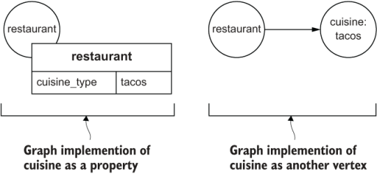
Figure 2.1 Two possible graph implementations for a restaurant’s cuisine

Put another way, the physical data model is largely a result of the queries we write. We know that, for some, this feels like putting the cart before the horse. Don’t you usually create the data model and then write the queries? Yes, we have done that many times and have painted ourselves into a corner with design mistakes more often than we would like to admit. The approach we take is designed to reduce that risk and to minimize the pain of data model changes.

Going back to the use of different terms for different parts of the process, the other reason for this goes back to our main point as stated at beginning of this section: we translate a real-world problem into a technical domain. We use the technical terms vertex and edge when working with a specific type of data engine, a graph database in this case. If we use a relational database, the technical terms become table and column. But data modeling starts with engagement with the business, with the users and their perspectives. The business and end users do not think in terms of vertices and edges, nor do they use these terms in their normal day-to-day tasks, and they shouldn’t. The process we describe here uses different terms, like entity and relationship, to remind us that the conceptual model is a tool for communicating requirements between the end users and the developers.

2.1.2 Four-step process for data modeling

Having defined our data modeling terms, this leads us to the data modeling process itself. The process uses the following four steps, and each step is covered in detail in its own section:

1. Understand the problem. We start in section 2.2 with a focus on the business or domain terms and language to ensure a clear understanding of the end user’s perspective. We’ll explore project goals to make certain that the domain and scope of the problem is clear. At the end of this step, we’ll have specified the common terms and the core access patterns of users.

2. Create a whiteboard or conceptual model. After understanding the problem and the language used to describe it, in section 2.3, we’ll move from text to a picture, focusing on drawing a diagram that makes sense to the business users and one that’s useful to the technical developers. We’ll define the conceptual model, which includes codifying the main entities and relationships between those entities. After completing this step, we’ll have a high-level picture of the problem domain from the business perspective.

3. Create a logical data model. In this step, covered in section 2.4, the technical implementers (that’s you!) combine the domain defined in the first step with the conceptual model from the second step to create the physical description of the graph data model. This includes defining the vertices and the edges, as well as specifying the properties on those.

   Most graph databases are schemaless, so once we define this logical model, we’re ready to begin working on our queries. If your chosen graph database requires explicit schema definitions (similar to defining tables and keys in an RDBMS), we’ll also look at those at this time. In either scenario, once we finish this section, we’ll have completed the data model for our social network use case.

4. Test the model. In section 2.5, we’ll verify that our developed model satisfies the defined problem, that the entities and relationships needed to answer our user’s questions exist, and that these are properly named. This step focuses on validating coherence in the three previous steps, where we moved from a textual description of the domain to a simple picture of the entities and relationships and, finally, constructed our model with vertices and edges. This is largely a matter of asking, “Does this make sense given the other steps?” and “Did we leave anything out which we established before?”

The first two steps in this process are a partnership between the business users and the technical development staff, first defining a common set of terms and then illustrating how those terms relate to one another in a simple diagram. For the last two steps, a technical team member takes the diagram and builds and tests the logical model that becomes the basis for implementation, as shown in table 2.1.

Table 2.1 Summary of the design process for developing a logical data model

Data modeling step	Participants	Tools	Output
1. Problem definition	Business, Developers	Domain, scope, business entities, functionality	Textual description of problem
2. Conceptual data model	Business, Developers	Entities, relationships, access patterns	Picture of entities and their relationships
3. Logical data model	Developers only	Vertices, edges, properties	Diagram of graph elements
4. Test the model	Developers only	Preceding steps	Coherence of the outputs of prior steps

For some of us with a highly structured mindset, we know that providing a four-step process to guide both this chapter and all future data development deeply resonates with our desire for a well-ordered world (and development process). But we also know that some “code-first cowboys” out there feel that four enumerated steps are three steps too many. Sure, we know that in many cases “code wins,” and that an 80% implementation is often preferable to a 100% design. But this book is not targeted at building toys. Instead, we aim to build production-level applications with highly connected data in complex domains.

We are not suggesting spending endless hours/days/weeks agonizing over the perfect data design before writing any code. Designs change just as quickly as the business can create new requirements, so yesterday’s perfection is tomorrow’s functionally incomplete application.

We know from experience that mistakes in the data design phase cause problems during implementation, and that these problems are significantly harder to fix at that stage. Don’t be deceived by the apparent simplicity of a graph or by the schema-lite/schemaless nature of some graph databases. Any implementation implies some level of written and tested code, and data that is loaded. As with any relational database project, design changes usually mean schema changes, which leads to code change and, likely, a data migration of some sort. All of these additional downstream effects have to be dealt with, and often with less mature tooling.

2.2 Understand the problem

Whether working in a large enterprise, a small company, or just on a side project, the first step in data modeling is understanding the problem, the domain, and the scope of the work we are addressing. In a large enterprise, this work may have already been done for us through some requirements document. In a small company or with personal projects, that is unlikely to be the case. In the end, it doesn’t matter if our project has a requirements document or not; it is up to us to have a sufficient understanding of the problem before beginning work on our data model.

In this section, we examine several types of questions we need to answer before we can develop our data model. Ideally, these sorts of questions are already identified in functional and business requirements before beginning the project. The goal of these questions is to define how users interact with the system so we can develop a logical data model that supports the users’ preferred access patterns.

Note If you already have a strong background in data modeling, feel free to skip this section and move on to the next. If not, then read on and learn about what you need to know to ensure that you understand the problem.

We’ve found that users are very clever. Even if your model doesn’t directly support their preferred access patterns, they find a way to make it work. But if they can’t find a workaround, then they stop using the tool. Think about that! Fail here and your application is abandoned. Now isn’t that a cheery thought?

While the questions vary by project, there are different categories of questions that help us gain a clear view of the problem. These categories include the following:

• Domain and scope

• Business entity

• Functionality

In the next few sections, we explore each of these types of questions, discuss why these are important, and provide some examples from our DiningByFriends application.

2.2.1 Domain and scope questions

Every problem can expand in infinite directions, so the more precisely we define the scope, the more likely we are to succeed. Domain and scope questions define the boundaries of the problem. If we make the domain too broad, then we risk not understanding its boundaries and may never complete the application. If we make the domain too narrow, then we may miss out on critical features and not provide sufficient functionality to our users. Properly defining the domain and scope of the problem you work on is therefore crucial to building a complete and functional application. The following sections provide example questions and answers to narrow the scope of the problem for our DiningByFriends app.

What will DiningByFriends do for its users?

DiningByFriends provides users with personalized restaurant recommendations. When using DiningByFriends, users have three main needs that the application must satisfy:

• Social network --Users want to connect with friends who are also using the application. This functionality is similar to the way people connect with friends on any social network such as Twitter, LinkedIn, or Facebook.

• Restaurant recommendations --Users want to create and look at reviews of restaurants and then get recommendations for a restaurant based on these reviews. This is the central service the app provides.

• Personalization --Users want to rate the reviews of restaurants to indicate whether the review was helpful or not. Then they want to combine these reviews with their friends’ ratings to receive personalized recommendations based on the restaurants their friends also like.

What types of information does the application need to record to perform these tasks?

To answer this question, DiningByFriends should include at least the following information:

• All the basic identifying information about users, such as a name and a unique ID, so people can find and connect with them on the social network. (In a real-world scenario, this would likely include many additional attributes, but we keep it limited for this example application.)

• Restaurant identifiers and details, such as the name, address, and cuisine, to provide location-specific recommendations.

• The text of the review, along with the rating and a timestamp of the rating in order to get personalized recommendations.

• Reviews need to include ratings of its helpfulness (for example, up/down thumbs) so that friends know if a user agreed or disagreed with those reviews.

Who are the users of our application?

We have one type of user for our application. This includes users of the application who connect with friends, enter reviews, and receive recommendations.

NOTE We know that nearly all complex applications have internal or system users of some sort. These can include system administrators, customer service personnel, and others responsible for the maintenance and operation of a complex technical solution. We have elected to ignore such requirements in an effort to streamline the design of the use case. We therefore only focus on the traditionally understood end user.

From the questions in this section, we now have a fairly clear picture of the problem domain and its scope, as well as a set of terms that make sense to the business or end users we want to serve. And we now know the critical items needed to construct a personalized restaurant recommendation: people (users), restaurants, restaurant reviews, and ratings of those reviews.

2.2.2 Business entity questions

This type of question identifies the business entities and relationships within our problem domain. Looking at artifacts such as a relational database schema, entity relationship diagrams (ERDs), or other architectural documentation often helps us obtain a sense of the structure, language, and terminology already in use. Our goal is to identify the fundamental building blocks of our application and how these are related to one another. The following sections provide a few examples of the business entity questions we might ask.

What sort of items or things does the application utilize?

The application works with people, reviews, and restaurants.

How do these items interact with one another?

• People write reviews.

• Reviews discuss restaurants.

• Restaurants serve one or more types of food.

• A person is friends with another person.

• People rate reviews.

What are the critical pieces of data you need to know about each entity?

While not an exhaustive list, here are some items we need to store:

• User data --First and last name to help identify users

• Restaurant data --Details such as names, addresses, and types of foods served

• Reviews --Descriptions of the users’ experiences.

• Ratings --Rankings of a review so that friends know if it is helpful or not

Graphs and graph data models derive much of their power from having well-defined relationships between entities, which is a change for those of us used to relational data modeling. A well-defined relationship in a graph requires not only a name for the relationship but also an understanding of how that relationship connects entities, as well as any potential attributes required to define the relationship. Therefore, it is critical to spend extra time exploring the relationships between entities, looking for potentially important interactions that are not immediately obvious. Looking at the answers, we often find a relationship and entity not called out specifically but hidden in the replies.

Exercise Do you see any hidden entities or relationships in the previous lists of questions about the business entities for our DiningByFriends app?

As we examine the list, we see a hidden relationship between a restaurant and the type or types of food served. In our restaurant recommendations application, it is highly likely that a user wants to search a specific type of food or cuisine to get recommendations. This desire means that it’s likely beneficial to make cuisine (Pizza, Chinese, Indian, etc.) an entity itself and to add a corresponding relationship between a restaurant and its cuisine.

2.2.3 Functionality questions

Questions concerning functionality reveal how our business entities interact, which represents the relationships between these entities. These questions start by exploring what the user might ask of the system or what problems users have that they want the system to solve for them. These problems determine both the questions that the user asks and, sometimes, the order in which they ask those.

When we get to the conceptual model in the next phase (section 2.3), we codify the functionality as access patterns. Later, we test our logical model (section 2.5) to see if it can provide the described functionality, or put another way, support the identified access patterns. The final use of functionality is in the actual implementation, when we build the queries for the system in chapter 5. The definition work we do in this step becomes the bedrock on which we build our application. In slightly more practical and graph-oriented terms, functionality definitions lead directly to the edges we define in our logical model and, likely, some of the properties for the edges as well. Let’s look at a few functionality questions for our use case.

How are people going to use the system?

Users create friendships with people they know, provide reviews, rate restaurants, and read and rate reviews submitted by their friends.

What questions does DiningByFriends need to answer for the user?

These questions about functionality fill in the details of how a user is going to interact with the system:

• Who are my friends?

• Who are the friends of my friends?

• How is user X associated with user Y ?

• What restaurant near me with a specific cuisine is the highest rated?

• Which restaurants are the ten highest-rated restaurants near me?

• What are the newest reviews for this restaurant?

• What restaurants do my friends recommend?

• Based on my friends’ review ratings, what are the best restaurants for me?

• What restaurants have my friends reviewed or rated in the past X days?

We now know what our users are going to do with the app and also what they are going to ask of it. In other words, this is a first pass at our queries using natural language. (Remember that this process is done with the business or end user and should be completely understandable by them.) As we mentioned at the top of this section, gaining this understanding of this information ensures that we model our data in a way that matches the users’ desired access patterns.

2.3 Developing the whiteboard model

The second step in our modeling process is to develop the conceptual or whiteboard model. We need to get a high-level diagram of what the schema for DiningByFriends looks like from a business perspective. This is our first tangible picture of the system, and it must be driven by the business view of the problem.

As builders, it is in our nature to solve problems, usually right away. But it is vital to take time to understand and define the business perspective of a domain. This accelerates our development process in the long run. Isolating what is most important to the business is crucial to making informed decisions and preventing unnecessary complexity and excessive rework.

2.3.1 Identifying and grouping entities

We develop our conceptual data model by first extracting the entities in our domain. As you’ll recall, entities refer to the things in our application domain and represent either physical items, such as people and places, or logical items, such as reviews and ratings.

Tip Start by looking for the nouns.

Once we locate the entities, we need to identify items that can be easily grouped into a single entity. When making these groupings, it pays to listen to the way business and other non-technical users discuss the problem. These users live this problem almost daily; if they use nouns interchangeably, signaling that the nouns are synonyms, then it is likely these can be combined into a single entity. For example, if we are working on an internal application and the business users mention user, employee, or client interchangeably, then we could probably group these nouns into a single entity within our conceptual model.

As a best practice, we should make all the names of our entities singular because each entity represents a single instance of that item. We know that there are those who prefer to use plural nouns for their entity-naming schemes, but we have found that singular names tend to be a better fit for graph data modeling.

Exercise Looking back at the answers in section 2.2, identify what you think the entities for DiningByFriends should be.

Looking at the answers, we find four entities for DiningByFriends:

• Restaurant --Represents a restaurant, which includes name and location.

• Cuisine --Describes the type of food served. This entity was not explicitly defined as one of the nouns but was found by listening to how the business described its needs.

• Person --Represents a system user, which includes the first and last name.

• Review --Actual review content, which includes the full review text and rating.

How does this compare to your list? If you have more, less, or a different set of entities, don’t worry. There is no one correct answer, and different people often come up with different solutions. We chose the entities in the list because we thought these were the highest-level items that could be derived from the information available, while still providing context to our problem.

Now that we have our entities, let’s put that “whiteboard” to use. We start our diagram with a box for each identified entity, as shown in figure 2.2.

Figure 2.2 Conceptual whiteboard diagram with our entities for DiningByFriends

2.3.2 Identifying relationships between entities

The entities we just identified represent the what in our data model. The next step is to determine the relationships or the how. Extracting relationships is similar to locating the entities, except instead of looking for the nouns in our answers to the functionality questions, we look for the verbs. The verbs describe how any two of our entities interact. Once we have identified the verbs, we need to provide names to describe the relationships. To name these, we take each verb and combine it with the entity names in the form noun-verb-noun or entity-relationship-entity to form a short, understandable phrase (Restaurant Serves Cuisine, for example).

Exercise Look for the verbs in our functionality questions and locate what you think the relationships in DiningByFriends should be.

Were you able to generate a list of relationships? It is a bit harder than finding the entities, isn’t it? Then again, this step is complicated by not having a user to interview. Here is our list along with the functional questions each relationship addresses (questions can appear more than once):

• Person-Friends-Person --This relationship helps construct the social network component of our app by allowing the application to answer user questions such as

  • Who are my friends?

  • Who are the friends of my friends?

  • How is user X associated with user Y ?

• Person-Writes-Review --This relationship enables us to construct the recommendation engine for DiningByFriends as the reviews serve as the underlying data to provide recommendations. This relationship allows the app to answer user questions such as

  • Which restaurant near me with a specific cuisine is the highest rated?

  • Which restaurants are the ten highest-rated restaurants near me?

  • What are the newest reviews for this restaurant?

  • What restaurants do my friends recommend?

  • Based on my friends review ratings, what are the best restaurants for me?

  • What restaurants have my friends reviewed or rated in the past X days?

• Reviews-Are About-Restaurant --This relationship allows our application to formulate our recommendation engine as these reviews need to be associated with a restaurant that the app recommends. Here’s a list of questions to consider:

  • Which restaurant near me with a specific cuisine is the highest rated?

  • Which restaurants are the ten highest-rated restaurants near me?

  • What are the newest reviews for this restaurant?

  • What restaurants do my friends recommend?

  • Based on my friends review ratings, what are the best restaurants for me?

  • What restaurants have my friends reviewed or rated in the past X days?

• Restaurant-Serves-Cuisine --This relationship allows us to provide some of the filtering capabilities for the recommendation engine, especially the ability to recommend a restaurant based on cuisine:

  • Which restaurant near me with a specific cuisine is the highest rated?

• Person-Rates-Reviews --This relationship enables our app’s personalization component by providing the information needed to tailor a recommendation to a specific user based on their friends’ reviews:

  • Based on my friends review ratings, what are the best restaurants for me?

  • What restaurants have my friends reviewed or rated in the past X days?

How does our relationship list compare to yours? As with entities, there is not one correct list. Many people go a step further and describe the attributes, or properties, of the entities and relationships. We shy away from this whenever we can because defining attributes this soon devolves into an exercise in bikeshedding (focusing on the comparatively trivial aspects of a problem instead of targeting the goal, which is to develop a high-level understanding of our application).

Although there is certainly a danger of “tyranny of the trivial” by spending too much time on properties, there is also the potential that useful details can come up in such a discussion. To mitigate the risk of losing those helpful details--details that can be used later, particularly in building the filtering and search components--we timebox the exercise by limiting ourselves to 10 or 15 minutes of discussion. During this time, we capture key points on Post-It notes, on a dry-erase board, or in a Google document, and drop these as a task in the backlog for later review and action.

Tip Don’t underestimate the power of a virtual “idea parking lot” for staying focused on the primary tasks at hand.

When it is time to put pen to paper to the conceptual model, we prefer a much simpler whiteboard--a box-and-arrow conceptual data model built with flowchart software such as Microsoft Visio or Lucidchart, or even with simple presentation tools such as PowerPoint or Google Slides--to a more defined methodology, such as Unified Modeling Language (UML). We build these flowchart models by representing the entities as labeled boxes and the relationships as labeled arrows. Doing this for DiningByFriends, we get the chart depicted in figure 2.3.

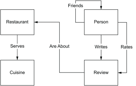
Figure 2.3 Our conceptual data model shows the entities (boxes) and relationships (arrows) for DiningByFriends.

We’ve found that both technical and non-technical users easily understand whiteboard models, which are intuitive. At this point, the target audience for this model is a business user, not a developer, so we want to stay away from thinking about the physical implementation. That will come soon enough.

2.4 Constructing the logical data model

Now we are ready to build our logical data model and translate those entities and relationships to the graph concepts of vertices, edges, and properties. The outcome of this process is another diagram, but this one contains sufficient detail to provide the necessary schema information for a developer to begin coding an implementation. In this section, we only work on the first use case in our application: the social network functionality. Later in the book we extend our data model for the other features. We start with social networking for several reasons:

• Our social network is the basis for how we eventually extend DiningByFriends for our recommendation engine and personalization features.

• The number of questions the social network answers is small enough to allow us to acquaint ourselves with the patterns and processes of graph data modeling.

• This network is the most straightforward, but it still retains several features, such as recursion and self-referencing edges, that enable us to highlight some of the unique abilities of graph databases.

To refresh our memory, the requirements for our social network provide the ability to connect with friends to see what they are reviewing. It addresses these questions for the Person-Friends-Person relationship:

• Who are my friends?

• Who are the friends of my friends?

• How is user X associated with user Y ?

Figure 2.4 shows the portion of our conceptual data model that we work on in this section. Because we use this part of the model throughout the rest of the chapter, we repeat this same diagram so that it is always readily accessible for you.

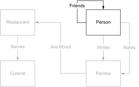
Figure 2.4 Conceptual data model for DiningByFriends with the relevant parts required for the social network highlighted

We start by showing the completed data model and work backward to show the patterns and processes we used to come up with this model. To begin, let’s examine the final graph data model for our social network, as shown in figure 2.5.

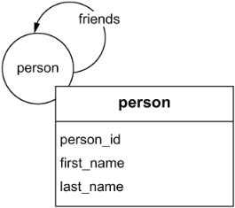
Figure 2.5 The logical graph data model for the social network for DiningByFriends

As figure 2.5 shows, the graph data model for this use case is one vertex with the label person, one edge with the label friends, and three vertex properties with the keys person_id, first_name, and last_name.

Note In some environments, keys and key-value pairs are called property names and name-value pairs.

Now that we know our end state, let’s see how we got there. There are four steps to building a graph data model from a conceptual model:

1. Translate entities to vertices.

2. Translate relationships to edges.

3. Find and assign properties to vertices and edges.

4. Check your model.

Wait...what does that say... “properties to vertices and edges?” Yes, you read that correctly. This ability for both vertices and edges to have properties highlights another fundamental difference between a relational database and a graph database. Because relationships are first-class citizens in a graph data model, both vertices and edges can have properties associated with those. While this addition might seem trivial, it is one of the more powerful aspects of a graph database because it opens up several useful data modeling options that we explore throughout this book.

2.4.1 Translating entities to vertices

The first step in creating our graph model is to identify all our vertices. Much of this work was done when we developed our conceptual model because the entities in a conceptual data model map almost directly to the vertices in a logical graph model. The creation of the vertices in our graph model requires two things:

• Identify all the relevant entities from our conceptual model

• Give the vertex a name in the form of a label to uniquely identify that type of entity in our graph model

To begin these two tasks, let’s glance at the social network section of the conceptual data model. Figure 2.6 presents this section, and then we examine each point in more detail.

Figure 2.6 The conceptual data model with the relevant parts required for the social network highlighted

Finding the conceptual entities

In our conceptual model, we located the entities Person, Restaurant, Review, and Cuisine. Now we need to narrow those down to only the entities required to answer the questions from section 2.3 for our social network functionality:

• Who are my friends?

• Who are the friends of my friends?

• How is user X associated with user Y ?

In this case, the questions refer to only one entity, Person, because “my friends” and “the friends” are both people. While there are other logical entities in the model (Review, Restaurant, Cuisine), these are not required for the app’s social networking, so we can ignore these for now. Although this is a simple example, this step will be more involved when we get to more-complex use cases in chapter 7.

As a general rule, we look for the entities in our application by looking for the nouns in our list of functionality questions. Because nouns represent physical or logical items, these frequently are the best indicator of which entities are required to solve the questions in the application.

Naming the vertex labels

Now that we have identified our entities, we need to assign each a label. A label in a property model graph categorizes or groups vertices that represent similar concepts. As has been observed by many prominent coders, there are only two hard things in computer science: cache invalidation, naming things, and off-by-one errors.1

Deciding on label names is not a trivial undertaking. A good label name is short, descriptive, and precise. As with properly naming variables in an application, if you do it well, the names add significant clarity and provide additive value when reading and working in the code. If you do it poorly, names can obfuscate their purpose and can be misleading. In software development terms, a label in a graph database is analogous to a class in object-oriented languages such as C++, C#, or Java: both contain a definition to explain how an object is structured and both can be used to classify like items together.

For the Person entity, the conceptual model also uses the entity name Person. Going back to our problem definition, let’s pretend that we often talk with the business and end users and find that there is an existing implementation using a relational database. In this feature-discovery fantasy, we see that the business users refer to that entity as both people and users. With different terms being used for the same entity, we decide that Person is the most descriptive name for this entity.

Important It is a best practice to make vertex labels singular because each vertex only refers to a single instance of an item.

We could have gone with the name User, but this is specific to one type of potential person within the application. While we currently do not have this requirement, we might need to represent other types of people, such as employees or owners, in the future. By choosing the more generic label of person, we can represent these potential future entities more easily without losing the type information in our current system.

Important It is also a best practice to make labels as generic as practical. While we will go into this in greater detail in chapter 7, a rule of thumb is that if we expect that we might need to represent other, similar concepts in the future, then it’s worthwhile to use a more generic term.

As with other databases, a consistent naming convention for label and property names is critical to the maintainability of an application. Consistency provides predictable behavior for developers and administrators. As developers, we find nothing more frustrating than inconsistent naming conventions in databases, and graph databases are no exception to this rule. For this book, we use lower_snake_case names and make all label names singular. Applying these best practices, we settle on the label person, as shown in figure 2.7.

Figure 2.7 Example vertex with the label person

Note It is generally a safe bet that each vertex in a graph database can only be associated with a single label. That is the approach of Apache TinkerPop, and it is the approach we take in this book. There are situations, such as modeling inheritance, where having multiple labels per vertex is appropriate. And some graph databases, such as Neo4j and Amazon Neptune, do support multiple labels per vertex. Be sure to understand your vendor’s capabilities before starting the data modeling process.

2.4.2 Translating relationships to edges

Now that we have identified and labeled our person vertex, it is time to define our edges. Edges are based on the relationships from our conceptual model. Defining edges takes a little more effort than finding the vertices. The edges in graph databases include features like directionality and uniqueness, which do not have direct counterparts in relational databases. Therefore, defining these relationships is more involved than just applying a name as you would do in a relational database. The four steps to defining an edge are

1. Identifying the relevant relationships from the conceptual data model

2. Naming the edge in the form of a label to uniquely identify that relationship in our graph data model

3. Assigning a direction to the edge by defining the start and end vertex types

4. Specifying the uniqueness of the edge by deciding on the number of times this edge can exist between two specific instance vertices

Finding the relationships

Recall from the conceptual model that the social network component includes a single entity, Person, but this particular entity has three relationships associated with it: Friends, Rates, and Writes. (Friends here is a verb.) Let’s look again at the functionality questions for the social networking we discovered while building our conceptual model:

• Who are my friends?

• Who are the friends of my friends?

• How is user X associated with user Y ?

All the questions revolve around how one person is connected to another as a friend. The Friends relationship is the only link from a person to a person vertex that’s required for our social network. The Rates and Writes relationships are not required because these reference an entity (Review) that is not required for this use case. Let’s see what our conceptual model looks like with the relevant sections highlighted in figure 2.8.

Because we were thorough when creating the conceptual model, this part of the translation to the logical model is almost trivial. If we missed a relationship and a corresponding edge, then that begins to surface as we evaluate the access patterns against the logical model in our test phase (more on testing in section 2.5).

Figure 2.8 Conceptual data model with the relevant parts required for the social network highlighted

Naming the edge labels

Now that we know that we need to represent the Friends relationship as an edge in our model, it is time to name it (step 2), just like we did with vertices. To decide on the edge label for our data model, we apply the same best practice naming rules: be concise, descriptive, and generic. By applying these rules, we get an edge with a friends label that starts at a person vertex and ends at a person vertex, as shown in figure 2.9.

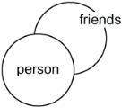
Figure 2.9 Adding a friends label connecting a person vertex to a person vertex in a loop

Don’t be alarmed that the edge is connecting back to the same vertex type. It is acceptable, even common in some models, for an edge to have the same vertex type at both ends. This is known as a loop. A loop edge is similar to a foreign key referencing the same table or a linking table that connects back to the original table, as in figure 2.10.

Figure 2.10 A loop in a graph data model is similar to a linking table in a relational data model. It references back to the original table.

Giving the edge a direction

Once we have a label for our edge, the next step is to give the edge a direction. By convention, the direction of an edge is described as being from one vertex, the out vertex, to another vertex, the in vertex. In figure 2.11, we see that the Bill vertex is the out vertex and the Ted vertex is the in vertex.

Figure 2.11 Example of data in a graph with an out vertex for Bill and an in vertex for Ted

In a good graph model, the vertex-edge-vertex combinations read as a sentence. In figure 2.11, we read the vertex-edge-vertex as Bill friends Ted. When looking at your label names and edge directions, don’t be afraid to reword the label or switch the direction of the edge to make the data model more understandable. The direction of an edge should complement the edge label to make a sentence that sounds natural (or mostly natural) and that fits the functional needs of the use case.

Consider the example of a simple graph, shown in figure 2.12. It tracks the cities people live in. There are two vertex labels, person and city, and one edge label, lives_in, between the vertices.

Figure 2.12 A sample graph with the schema, person-lives_in-city, and the instance data, Jane-lives_in-Chicago

In figure 2.12, we see both the schema of our graph and the instance data (the graph of the data stored). Looking at the instance data graph, we see that Jane lives in Chicago. Looking at this data, it makes logical sense and reads fluently. If we reverse the direction of the edge so that the in vertex is a person and the out vertex is a city, then the instance would read as Chicago lives in Jane. As cities don’t live in people, this sentence no longer makes sense. So, what can we do to make this sentence make sense? The simplest solution is to reword the edge label to something that makes the sentence more understandable, such as is_residence_of, as shown in figure 2.13.

Figure 2.13 Reworded graph with the edges is_residence_of for both schema and instance data

Now if we read the instance of the reworded graph, we see that the sentence, “Chicago is residence of Jane,” makes sense. Returning back to our DiningByFriends model, because our friends edge connects a person vertex to a person vertex, the direction is irrelevant. Figure 2.14 shows that the start and end vertex labels are identical.

Figure 2.14 The friends edge, now with an added direction pointing from a person vertex to a person vertex

It certainly simplifies things in social networking queries when the edge direction, while specified, is not consequential, but don’t expect to see this often! This situation is very uncommon.

Determining edge uniqueness

The final step to address when defining edges is uniqueness. Edge uniqueness describes the number of times an instance of a vertex is related to another instance of a vertex with an edge having the same label. Whew, that definition is a mouthful, so here’s another way to define this concept: uniqueness describes what is an allowable number of edges of a given label between two vertices. That is still a bit abstract, so let’s take a look at an example that demonstrates what we mean by edge uniqueness.

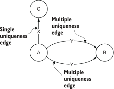
Figure 2.15 Entities A and C have one single uniqueness edge or relationship with each other. Entities A and B are connected more than once, having multiple uniqueness edges.

In figure 2.15, vertex A is connected to vertex B by edge Y more than once, so edge Y is a multiple uniqueness edge. Vertex A is also connected to vertex C by edge X, but it is only connected one time; thus, edge X is a single uniqueness edge.

Why does edge uniqueness matter? Let’s use a simple movie example as shown in figure 2.16 to see why. This graph consists of three people (entities)--Bob, Joe Dante, and Phoebe Cates--and shows the relationships (edges) to the movie Gremlins (also an entity).

Figure 2.16 A simple graph with four entities, or vertices, and three edges

In our Gremlins graph in figure 2.16, we have four vertices (three person’s and one movie) and three edges (watched, acted_in, and directed). Each person in the graph is connected to the movie vertex using one of the three edges. In this example, the following relationships exist:

• Bob watched Gremlins.

• Phoebe Cates acted in Gremlins.

• Joe Dante directed Gremlins.

Let’s begin by examining the directed edge in our graph. Remember, we are looking for what is the allowable number of edges of a given label between two vertices.

We can all agree that a person (Joe Dante) can only direct a movie (Gremlins) once, so the directed edge has single uniqueness. This does not preclude Joe Dante from having multiple directed edges because he also directed Gremlins 2, or mean that Gremlins could not have multiple directed edges going into it. It merely enforces that there can be only a single directed edge from Joe Dante to Gremlins.

Single uniqueness is, in fact, significantly more common than multiple uniqueness. As a rule, assume single uniqueness and think about multiple uniqueness only when there is a specific requirement dictating multiple instances of the same edge between two vertex instances.

When does an edge require multiple uniqueness? Take the example of the watched edge; we can all agree that it is possible, and certainly likely, that a person would watch the movie more than once. As a result, there would be multiple watched edges between Bob and Gremlins as shown in figure 2.17.

Figure 2.17 Multiple uniqueness demonstrated with multiple watched edges between Bob and Gremlins.

Multiple uniqueness is less common than single uniqueness. But it is useful when the same relationship can exist between the same two distinct items multiple times, such as tracking the times a person has ordered a product or documenting connections between items on the internet.

Now, let’s review the last edge in our movie graph, the acted_in edge, and see what its uniqueness should be. Based on the definition of uniqueness (What is the allowable number of edges of a given label between two vertices?), what do you think its uniqueness should be?

We would probably only ever have a single acted_in edge between a person and a movie, so it would have single uniqueness. But if we think about people acting in movies, it is possible that a user acts in the same movie multiple times in different roles. Examples with Eddie Murphy or Tyler Perry come readily to mind. How would we go about modeling the requirement to store the fact that a person was in a movie in more than one role?

In figure 2.16, we could allow for multiple acted_in edges between a person and a movie, but there is no way to distinguish the role associated with that acted_in edge from the role associated with another acted_in edge. If we were to change the acted _in edge to have a role property, then we could see that Eddie Murphy acted_in The Nutty Professor in two separate roles, Sherman Klump and Buddy Love. We would also be able to identify the role that is associated with each edge, as shown in figure 2.18.

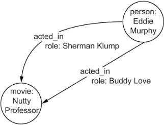
Figure 2.18 Adding a role property to the acted_in edge creates a mutiple uniqueness edge to express the fact that Eddie Murphy acted in multiple roles in the movie Nutty Professor.

If we add the role property as shown in figure 2.18, then the acted_in edge would be considered a multiple uniqueness edge. This is just one example of how you can use the uniqueness of your edges to represent information in your domain.

Returning to our graph data model for DiningByFriends, what would the correct uniqueness of the friends edge be? We could say that it is a single uniqueness edge because a person can only be friends with a person once. How do we know if we have the right edge uniqueness? To answer this question, let’s first look at how incorrect uniqueness can affect an application. Improper uniqueness usually appears in one of three ways:

• Too little data returned

• Duplicated data returned

• Poor query performance

Important Incorrect edge uniqueness is one of the most common problems in graph data modeling, and it is frequently a root cause of query issues.

The first symptom of incorrect uniqueness is that too little data is returned from a query. This occurs when we have an edge with single uniqueness that really should be multiple. In this scenario, the query returns only the first edge saved or the last edge saved. The exact response returned depends on how the database handles data concurrency. But either way, it’s incomplete.

The second symptom, having duplicated data returned, occurs when we have multiple uniqueness edges but we should only have one. In this scenario, our application incorrectly retrieves data for multiple edges on each query because multiple edges exist between two instance vertices. Because we can have multiple edges with the same label between any two vertices, each time our application saves an edge between vertex A and vertex B, for example, a new edge is created. Over time, this means that we end up with a collection of many edges when we might have intended for only a single edge between vertex A and B to ever exist.

The third symptom of incorrect edge uniqueness is harder to diagnose because it appears as poor query performance. This can, of course, be caused by many things. But most often having a multiple uniqueness edge instead of a single uniqueness edge is what causes poor query performance, because the database has to do more work to return the data for a query with multiple edges. We discuss more about debugging and troubleshooting query performance in chapter 10, but let’s quickly look at why incorrect uniqueness causes a problem.

In the earlier Gremlins movie example, if the directed edge had multiple uniqueness, it would be possible that an incorrect traversal could create five directed edges between Joe Dante and Gremlins. If we run a query to return all the movies that Joe Dante has directed, which it does using all of the directed edges connected to Joe Dante, it requires the database to do five times the work because there are five times the edges to traverse between the two vertices shown in figure 2.19. And this can cause a noticeable performance impact to both your application and the database!

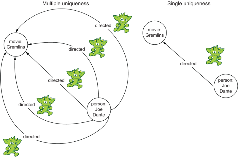
Figure 2.19 The comparative amount of work required for multiple uniqueness edges versus single uniqueness edges

If we continue with the extra edges example and imagine that we move out further in our graph, from the movies to the actors which Joe Dante directed, we can quickly see how this seemingly simple oversight exponentially increases the number of vertices and edges we traverse. The error in the directed edges would result both in repeated movies and in repeated actors. The good news is that there are a few ways to mitigate this problem at query time, which we cover when we start writing queries in chapter 3. But the best way to prevent this problem is to properly design the data model to reflect the correct uniqueness of the edges.

Some graph databases, such as DataStax Enterprise Graph and JanusGraph, set the uniqueness of an edge explicitly as part of a schema definition. But many other graph databases do not define schema explicitly, so there is no way for the database to enforce a uniqueness constraint. This schemaless approach of some graph databases means that we must write application logic to enforce this uniqueness within the application.

2.4.3 Finding and assigning properties

Now that we’ve created the structure of our graph model, composed of the vertices and edges, it is time to define the properties and assign these to the vertices and edges. Properties in a graph data model are key-value pairs that describe a specific attribute of a vertex or edge.

Before we can assign the properties to edges and vertices, we first have to decide

• What properties are required?

• How we are going to name them?

• What is their data type?

To answer these questions, we need to consider what we know about the domain as well as our conceptual data model to decide what information needs to be stored.

Note When migrating an existing system, it is beneficial to reference the data model for that system as a blueprint. Data models have matured over the years and so provide a rich perspective on the necessary data requirements for an application. If you are developing a greenfield application unconstrained by parameters set by prior work (such as we are with DiningByFriends), then now is the time to sit with the technical and non-technical people to determine what the specific data fields, names, and data types should be.

The first place we look for the properties is, once again, in our list of functionality questions for our social networking use case. If you remember, these are

• Who are my friends?

• Who are the friends of my friends?

• How is user X associated with user Y ?

Based on these questions, we can see that we need to store the first_name and last _name for a person to identify who our friend is. We can also assume that we are going to need a unique identifier of each person (person_id) to differentiate between people with the same name. Without this additional attribute, we are unable to discern one John Smith from another John Smith. Adding our properties to our current data model, we get the model in figure 2.20.

Figure 2.20 Our social network graph data model with the properties added (shown in the box)

In this case, we did not add properties to an edge because all the required attributes (person_id, first_name, last_name) describe the person, not the friends relationships between people. However, adding properties to edges is common, and we will have a chance to do so in our DiningByFriends model in chapter 7.

At this point in the process, if you chose to use any of the schemaless graph databases that exist on the market, then you are complete. But if you are using a database that requires the schema to be explicitly specified, then you have one additional step: translating your logical data model into the physical data model required by your chosen database. The actual mechanics for how this is done are specific to each database as each tool has its own unique definition language to describe the physical graph data model. Due to this lack of standardization across graph database vendors, we recommend reading the documentation for your chosen tool to complete this step.

2.5 Checking our model

The last step in creating our logical data model is to validate that we can answer the questions for our social network use case and that the model we built, shown in figure 2.21, follows best practices for graph data modeling.

Figure 2.21 The final logical graph data model for the social network DiningByFriends use case

Looking at our questions, can we answer these using our graph data model?

• Who are my friends? We can answer this question by starting at a specific person found by person_id and traversing the friends edge to see all of their friends.

• Who are the friends of my friends? We can answer this question by starting at a specific person found by person_id and traversing the friends edge, and then traversing the friends edge again to see all of the friends of my friends.

• How is user X associated with user Y? We can answer this question by starting at a specific person found by person_id and traversing the friends edge until we either have no more friends edges to traverse or we traverse to the destination person.

  Later in this book, we discuss precisely how to achieve this sort of query, but be aware that this sort of unbounded recursive query is one of the most compelling use cases for graph databases.

Now that we have a validated model, there are a few additional best practice checks to make sure that our data model provides a solid graph model:

• Do the vertices and edges read like a sentence? Yes. While this is not an absolute requirement, it is an excellent general check to verify that vertex labels represent the nouns in your model and the edge labels describe the actions or verbs in your model.

• Do I have different vertex or edge labels with the same properties? No. In this case we only have a single vertex and a single edge label. In a more complex model, as we see later in this book, this check is a helpful way to validate that you have made your labels generic enough.

• Does my model make sense? Yes. While this step can seem like an obvious check, it does pay to take time to step back and double-check that your graph data model has not strayed too far from your conceptual data model and that it makes sense for the problem that you are solving.

In this chapter, we built our data model for our social networking use case and validated that it makes sense for our problem. In the next chapter, we are going to start querying our database to answer the questions for our social network use case.

Summary

• Strong, early investment in understanding the problem, use cases, and common domain terminology are the foundation of building a good data model. This also reduces the risk that you’ll need to radically change the design later.

• A conceptual data model provides an overarching view of the scope, entities, and application functionality from the point of view of a business user.

• Translating a conceptual data model to a logical data model requires four steps: translate entities to vertices, translate relationships to edges, assign properties, and check the model.

• Translating entities to vertices involves identifying the required conceptual entities, creating corresponding vertices, and providing those vertices with a label that is concise, descriptive, and generic.

• Translating relationships to edges consists of identifying the required conceptual relationships, creating corresponding edges, labeling each edge, assigning a direction to each edge, and determining the edge uniqueness.

• Edge uniqueness defines the number of times an instance of a vertex can relate to another instance of a vertex with an edge with the same label. Incorrectly identifying edge uniqueness is a common problem in graph data modeling, which causes data and performance issues.

• To validate a graph data model, verify it against the requirements and conceptual model, check that the vertex and edge labels read like a sentence, and ensure that the model does not have duplicated edge or vertex types. Finally, perform a “gut-check” to see that the model makes sense.

---

1.The exact source for this bit of developer humor errors is not available, but it’s generally attributed to Tim Bray, Phil Karlton, and Leon Bambrick.