I HVAC control systems

I. I Basic concepts

It is not frequently acknowledged that heating, ventilating and air conditioning (HVAC) systems present one of the most challenging situations to deal with from the point of view of control. Swings in day-to-day, week-to-week and season-to-season energy demand together with the infinitely complex combination of user needs at the human interface contribute to a highly non-stationary ‘environment’ within which control takes place. It is little wonder then that much of HVAC control is about compromise; a compromise that usually amounts to reasonable comfort at minimum energy use and cost.

HVAC control in common with all process system control requires the governance of two distinct actions; those of switching or ‘enabling’ and regulating or ‘adjustment’. Switching in the majority of applications amounts to ensuring that the plant is available at certain times of the day (generally, those times of the day in which a building is in use). This will be essentially clock-based, occupancy-sensor-based or indeed based on some other logical two-state condition such as an alarm state. Regulation, which is what this book in essence is about, amounts to ensuring that the plant capacity is matched to the demands placed upon the system.

Let us consider some basic concepts of HVAC control. Figures 1.1, 1.2 and 1.3 show three quite contrasting ways of controlling the output of a simple heat exchanger. The actions of these three systems are quite different.

Under analogue control, the controller positions the valve anywhere between fully open and fully closed (Figure 1.4) using a smooth continuous signal from the controller. Control is defined in terms of a reference condition or set point (r) and a proportional band (p) which represents the range of the controlled condition for which the output of the controller is proportional. Figure 1.4 for instance shows that the valve will settle at the set point at 50% of its range and, during fluctuating conditions, the temperature will drift either side of the set point until control action restores its value at the latter. This was the predominant method of HVAC system control until the early 1980s and still exists today in the form of mechanical direct-acting control devices. For example, the ‘thermostatic’ radiator valve (TRV) is one case of this type of control.

Under thermostatic control, control is a two-state process. The thermostat is a switching device and positions the valve periodically in either a fully closed position or a fully open position; there are no in-betweens. Control action is defined in terms of a set point and dead band (d) which represents a band of inactivity the limits of which form switching events (Figure 1.5). This method of control is widespread; there are numerous examples in the home such as the domestic iron and the portable electric fan heater. It has the advantage of achieving reasonably effective control with great simplicity but the disadvantages of a fluctuating controlled condition (within the limits of the dead band) and the frequent switching of equipment which in some cases can cause excessive wear on components. For these reasons it is not used commonly in the UK for conventional HVAC control but is used widely for domestic heating, unitary air conditioners and small-scale atmospheric boilers.

Figure 1.1 Analogue control.

Figure 1.2 Thermostatic control.

Figure 1.3 Digital control.

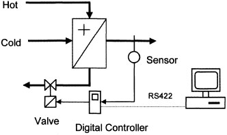
Figure 1.4 Proportional control action.

Figure 1.5 Thermostatic control action.

Figure 1.6 Typical analogue and digital control signals.

Whether networked or stand-alone application-specific, this type of control is now the predominant method for conventional non-domestic HVAC systems and plant.

We will now move on to take a look at some of the established applications of HVAC control.

1.2 HVAC control strategies

Constant-volume air handling

Figure 1.7 shows the general arrangement for the four-channel control of an air handling system serving one zone in which the four channels control, in sequence, heating → heat recovery → fresh air (‘free’ cooling) → chilled water-based cooling.

Note that the heat recovery is optional and would only tend to be used in this application when the minimum fresh air in total air handled is high due, for instance, to high occupancy density in the zones served by the air handling system. Note also that the controlled condition becomes supply air temperature in situations where the air handling system’s function is to provide pre-conditioned air to rooms or zones which themselves have local sequenced heating and cooling control.

Operation The controlled condition is the space temperature, θ_r. It is usual to measure this in the return air duct, provided that there are no intervening heat gains, such as light fittings, in the return air path. The return air will be well-mixed and the temperature sensor at the higher in-duct air velocities will tend to be more responsive than in the comparatively still air conditions of the space. For space or room temperature control, the manipulated variables will be:

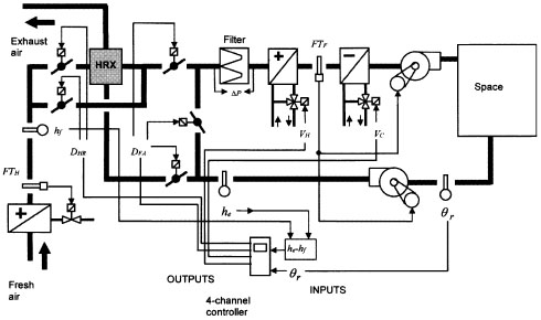
Figure 1.7 Control for constant-volume air handling.

During very warm summer weather, the fresh air damper will be fully open and the heat recovery face and bypass dampers positioned for full bypass in order to achieve ‘free cooling’. The limit to free cooling is reached when the fresh air intake enthalpy exceeds the enthalpy of the return air at a point downstream of the return air fan, a condition that takes place during the peak summer season in the UK though will often be short-lived. At this condition, it is necessary to signal to the fresh air damper a return to its minimum position and for the heat recovery face and bypass dampers to reposition so as to allow full heat recovery (which will now, in effect, provide pre-cooling of the fresh air from the cool building exhaust air). Enthalpy sensors h_e and h_f provide this and most control system manufacturers will permit additional plug-in modules for their multi-channel controllers to achieve these summer reset conditions. In the arrangement shown, when h_e – h_f produces a negative signal, the reset conditions described are enacted.

To provide frost protection, there are two features. Firstly, the heat recovery heat exchanger (if present) is protected from icing during very cold weather by an upstream frost coil on the fresh air side. Because of the highly temporal nature of calls on the frost coil, a simple thermostatic control through a two-position two-port control valve is usually sufficient. Frost thermostat FT_H provides for this. Secondly, should any primary heating plant such as central boilers or pumps fail, all coils in the arrangement are vulnerable to freezing of their respective water contents during very cold weather, especially the frost coil itself. To provide last-line protection against this, frost thermostat FT_F acts to trip both fans (a further precaution might be to provide a two-position isolating damper at the fresh air intake which coincidentally closes in these conditions thereby eliminating any natural draught through the plant when idle). Typically, FT_H would have a set point of 5°C, and FT_F, 3°C.

Sequencing Figure 1.8 shows the sequencing of this arrangement. Essentially, sequencing ensures that all control actions are mutually exclusive. From a very low controlled condition value, heating modulates as heat recovery is sustained at maximum, fresh air is a minimum and cooling is off. With the controlled condition value rising, the heating eventually reaches its off position. Heat recovery is then allowed to modulate with minimum fresh air and cooling off, and free cooling is allowed to proceed when the heat recovery reaches its off position. Only when maximum free cooling is effected is the chilled water cooling allowed to modulate at the high controlled condition value. By this sequence of events, minimum energy use is assured.

Dead zones may be programmed into the settings of each control channel, since each channel will be allocated a band of the control variable value within which it is active. A dead zone for instance between a heating and cooling action can help to ensure not only the mutual exclusivity of heating and cooling, but also that a gap exists between winter heating set point and summer cooling set point thereby minimising energy use throughout the seasons.

Figure 1.8 Sequencing for constant-volume air handling.

Variable-volume air handling

Figure 1.9 shows the general arrangement for variable-air-volume air handling (VAV) in which a number of zones or rooms are served (shown this time without the heat recovery option). Many of the principles of the previous case are applicable here as far as thermal control is concerned but, in essence, the supply air temperature becomes the controlled condition.

Operation There are a number of essential features and some optional features shown in this arrangement. First the essentials.

Figure 1.9 Control for variable-air-volume air handling.

There are two optional features shown in Figure 1.9.

Sequencing Temperature control for the arrangement of Figure 1.9 is very similar to that of the constant-volume case and is shown in Figure 1.11.

Supply fan control is governed by the static pressure sensor, P, which in turn is influenced by collective VAV terminal device activity. The VAV terminals will never shut off completely but will always pass sufficient air at turndown to ensure that minimum fresh air and reasonable air distribution in the space are maintained. Most practical systems will not turn down below 25%. Because a conventional VAV supply fan will seek to maintain a constant in-duct static pressure, fan power will be proportional to volume flow rate which, in turn, will be proportional to the cube of the speed. It follows that at 25% volume turndown, the supply fan will need to run at 63% of its design-rated speed at which point 25% of fan power will be drawn. Thus practical speed range is limited in these systems. The use of terminal-regulated air volume (TRAV – Hartman, 1993) obtains more fan power saving than in conventional VAV by allowing duct pressures to fall while VAV terminal dampers remain open, through the use of terminal box feedback. See also Li et al. (1996), Tung & Deng (1997) and Englander & Norford (1992).

Figure 1.10 Supply temperature set point schedule.

Figure 1.11 Temperature control sequencing for variable-volume air handling.

Room heating

Two strategies for the control of space heating in a room are considered in the following.

Compensated heating

This is a very common method of heating control and is, in effect, a form of feedforward compensation – a method discussed in detail in section 4.3. Figure 1.12 shows the arrangement for base compensation with external temperature and supplementary compensation with solar intensity and wind speed.

Operation Control is with respect to the heating flow water temperature, θ_wf. The control valve in this case is connected to mix with respect to the heating system (and divert with respect to the heating source) with a pump in the mixed flow. The controller seeks to maintain the flow water temperature at a set point which is reset from the external temperature, θ_o, via the reset module, RM, as illustrated in Figure 1.13. Optionally, set point scheduling can be further compensated with solar intensity (I_s) and/or wind speed (c_w).

The balance point temperature is that value of prevailing external temperature at which a combination of heat gains to the building and its thermal capacity are such that the building is in a state of thermal equilibrium. The balance point value will vary from building to building but a reasonable typical value is 15°C. This method of control has the advantage of being inexpensive in that, in theory, it can satisfy control for an entire building with temperature compensation, or an entire orientation of a building with temperature and solar compensation plus optional wind-speed correction. In practice, however, the method is seriously flawed since, even with full weather parameter compensation, internal casual heat gains are ignored leading to the possibility of over-heating (and consequential energy wastage).

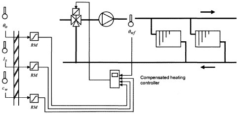
Figure 1.12 Compensated heating.

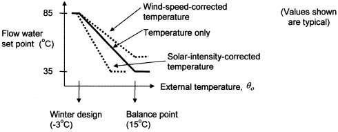
Figure 1.13 Typical compensated heating schedules.

Feedback heating control

The conventional method which eliminates the over-heating tendency of the previous system requires a control loop for each room or group of similar rooms. Whilst more costly, feedback control provides the only solution for potentially good control and energy efficiency. The (three-port) control valve in this case is connected to divert with respect to the heating system using a single pump, as shown in Figure 1.14. An alternative, which is beginning to become popular with some practitioners, is to use two-port modulating valves and a variable-capacity pump.

Sequenced room heating and cooling

The need to sequence heating and cooling in the thermal control of a space arises in many situations, most commonly:

Figure 1.14 Feedback heating control.

Sequenced feedback room control

Figure 1.15 depicts the arrangement for the constant-volume case, which is typical. A dead zone in the control sequence for this arrangement will ensure a gap between seasonal control set points. This is desirable to minimise heating and cooling energy use (e.g. 20°C winter, 24°C summer) – see for example Boyens & Mitchell (1991) for a treatment of minimised cost of operation with reference warm air heating plant. Figure 1.16 shows the typical control sequence.

Figure 1.15 Sequenced room heating/cooling.

Figure 1.16 Control sequence for room heating and cooling.

Cascade room temperature control

In the previous case, there are advantages in control quality and response if the supply temperature is ‘cascaded’ from the room temperature by resetting the set point of the former from the latter. Supply temperature therefore becomes the controlled condition but room temperature is fed forward and fully participates in the control. With this strategy, disturbances that result from plant interaction can be eliminated before they disturb the room condition, leading to a smoother response in the latter. This method is therefore often used in close control applications. Figure 1.17 shows the arrangement and Figure 1.18 gives a typical schedule for the reset module, RM.

Humidity and air quality

Year-round humidity control is generally only considered for close control applications – see for example Atkinson & Martino (1989), Mamula et al. (1989) and Clemens (1996). Many humidity and air quality control schemes will require the use of signal privatisation. We will consider each in turn.

Figure 1.17 Cascade room control.

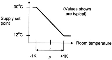
Figure 1.18 Typical reset schedule for cascade room control.

Humidity control

Steam humidification has become the principal choice today because of the potential for Legionella propagation in spray humidifier systems. In fact steam humidification offers one major advantage over spray humidification in any case; it can be readily modulated.

Dehumidification is less straightforward because, in comfort air conditioning at least, it is effected by condensing action at the cooling coil; but the cooling coil also has a role to play in temperature control. This dual role for the cooling coil leads to temperature and humidity control variables becoming ‘coupled’ – something which will be given special consideration in Chapter 6. Meanwhile there are two practical methods for tackling combined temperature and humidity control in full air conditioning systems.

Operation In winter a need for humidification and heating will exist and, accordingly, heating valve V_H and steam humidifier valve V_S will be sanctioned by the respective channels of the two controllers. In summer, the heating and steam humidifier valves will be closed and a need for cooling and dehumidification will exist. The signal priority module (SPM) receives dehumidifying and temperature control signals from the respective channels of the two controllers and selects the larger of the two signals for onward transmission to the cooling valve, V_C.

Sequencing Temperature sequencing is as before (Figure 1.16) and the humidification/dehumidification sequence will typically follow the pattern given in Figure 1.20.

Figure 1.19 Sequenced room heating/cooling/humidity control.

Figure 1.20 Room humidity control sequence.

Indoor air quality control

Control over indoor air quality (IAQ) generates some interest today since, inter alia, the possible link between ‘sick building syndrome’ and air quality was established in the 1980s. In HVAC plant, IAQ is effected by diluting sources of contaminant and ‘used’ air with fresh air. In situations where mixing dampers are in use it is necessary to prioritise the fresh air damper control with respect to free cooling demand and IAQ demand. The latter is established using either a selective gas sensor (e.g. carbon dioxide – see Warren & Harper, 1991) or a non-selective IAQ sensor (more about these in section 2.1). Figure 1.21 shows a possible arrangement.

Operation The temperature control sequence follows the now familiar heating → damper (free cooling) → cooling pattern. For air quality control, an air quality signal is generated by sensor q_r and the IAQ controller determines a damper signal based on this. The signal priority module (SPM) compares this signal with the coincident damper signal generated for free cooling and feeds forward the larger of the two signals for damper positioning.

Primary plant

Control of single units of primary plant, such as boilers, chillers and heat pumps, tends to be quite simple, based on a single- or dual-stage thermostat (e.g. for high → low → off control of a boiler). With such control, the only area of real concern lies in switching frequency; a rapid switching rate will tend to lead to wear on components with consequential maintenance problems. A judiciously sized buffer store can relieve this problem. For example, Wong & James (1990) report on the design of buffer stores for chilled water plant. See also Kintner-Meyer & Emery (1995) and Braun et al. (1989).

From the point of view of control, the real interest lies in multiple arrangements of primary plant where sequencing becomes an issue. Whilst there are various strategies for sequencing this type of plant, the common premise is to ensure that the minimum number of active units are on-line at any one time. This ensures the minimum use of energy through the operation of the plant as high up its efficiency profile as the prevailing demand allows.

Figure 1.21 Sequenced room temperature and air quality control.

Stepwise control

Examples include atmospheric heating boilers with on:off or high:low:off firing combinations such as modular boiler packages and small- to medium-scale refrigeration and heat pump systems with cylinder-unloading control.

Under stepwise control, a permanent offset in flow water temperature arises because at any one time there will be a mismatch between what the heating system wants and what the plant can supply. The size of the offset will depend on the number of step stages or the step resolution. For example, three four-cylinder refrigeration machines with individual cylinder unloading offer 12 steps of capacity. Assuming equal capacity steps, the resulting control of chilled water for a circuit with control band equal to its design temperature difference of 5K will operate with a minimum offset with respect to set point of 5/12 = 0.42K. This is quite tolerable, but three single-stage machines then slip to a minimum offset of 1.67K, which may not be acceptable in some cases. For this reason, the control sensor is often placed in the water return connection to the plant where the signal tends to give a better reflection of the demand from the system.

Figure 1.22 gives a typical arrangement for a stepwise multiple boiler plant with high : low : off burners (note that many of the principles apply equally to stepwise refrigeration plant).

Figure 1.22 Stepwise multiple boiler control.

Operation The controller generates a control signal based on the signal from the return water temperature sensor, θ_wr. The size of this signal determines how many stages of boiler burner activity are stepped in. Generally, control in these arrangements will take place within a proportional band equal to the design circuit temperature difference with set point at the mid-position. A simple proportional controller is used since, with step offsetting, it is argued that it would be counter-productive to use anything more sophisticated (CIBSE, 1985). For example, a hot water heating system with a design flow water temperature of 80°C and return water temperature of 70°C will have a (return water) temperature set point of 75°C and a control proportional band of ± 5K. Hence at 70°C, all boiler stages will be at high fire and at 80°C all stages will be off. This simple scheduling approach is common but ‘near-optimal’ performance can be obtained using heuristic schedules (Zaheer-uddin et al., 1990).

As each boiler is brought off-line, the motorised isolating valve (MIV) and boiler shunt pump are positioned ‘off’. This prevents energy wastage by circulating hot return water through the idle boiler waterways but generates disturbances in overall circuit flow rate for which there are various remedies. One method is to oversize the primary circuit by 15–20% and include a large-capacity balancing header to which the various sub-circuits are connected.

Each boiler has a high limit trip thermostat (HLT) which is usually a feature of the integral controls provided by the boiler manufacturer. This will be set typically at 90–95°C for hot water heating operating at a nominal flow temperature of 80°C. Another common option is to locate a corrosion-protection thermostat in the return water connection to each boiler with a local bypass pipe and diverting valve around the boiler. This allows the shunt pump to short-circuit water around the boiler waterways immediately prior to bringing the boiler on-line, thereby rapidly heating the boiler waterways and preventing cool system return water from forcing flue gas dewing at the rear of the combustion chamber which can lead to corrosion. The boiler is then offered on-line as soon as the corrosion thermostat is satisfied.

Sequencing Figure 1.23 gives an example of the sequencing pattern for the arrangement of Figure 1.22. In the firing sequence shown, boiler 1 is the lead boiler (i.e. the first called), boiler 2 is the first lag and boiler 3 the second lag. An important feature of good sequence control for multiple primary plant is the ability of the control system automatically to rotate the lead boiler periodically to ensure equal use of the available plant.

Modulating primary plant

Modulating control of primary plant has, until recently, mainly been restricted to large-capacity plant; mostly in the multi-MW capacity range – see for example Lewis (1990). More recently, advances in variable-speed drives and burner technology have resulted in some manufacturers developing modulating control for lower-capacity plant. Under modulating control, it is possible to match plant capacity with system demand at all times, leading to more precise control. The plant remains on-line continuously except for periods of very light load and this prevents the stresses associated with frequent switching from ‘cold’ inherent in on:off controlled equipment. Examples of modulating primary plant include variable-speed drives in rotary compressor-driven refrigeration and heat pump plant, inlet guide vanes in centrifugal refrigeration plant, and variable air/fuel controls in pressurised fuel burners associated with boiler plant.

Figure 1.23 Typical stepwise boiler sequence.

Operation For water-cooled chillers, the usual objective is to maintain constant flow rate and constant temperature condenser water conditions at each condenser in order to maintain stable condensing gas pressure. In Figure 1.24 this is achieved with a three-port valve connected to mix warm return water with cool flow water from the source (cooling tower or naturally occurring source). The set point of the flow temperature, θ_wc, will typically be a little above summer design wet bulb temperature (e.g. 30–35°C for UK conditions) for cooling tower applications. For air-cooled machines, each condenser will be equipped with one or more variable- or stepped-speed propeller fans which adjust according to a signal, typically, via a pressure sensor in the condenser.

On the evaporator side, note that the arrangement shown is a series connection. There are certain advantages with this, in particular in maintaining stable overall circuit flow conditions irrespective of the number of machines on-line and there are also performance advantages due to higher evaporating pressures in the first-pass machine.

Figure 1.24 Typical multiple modulating chiller çontrol.

As to capacity control, since with modulating plant a precise balance between refrigeration delivered and that demanded by the system can be assured, the temperature sensor, θ_we, is located in the flow. The stepper in this case is responsible for switching each machine on- and off-line as well as to relay the appropriate positioning control signal from the controller.

Sequencing Figure 1.25 shows a possible sequence in which, again, the essential philosophy is to minimise the number of on-line machines at any one time. Few modulating machines are capable of modulating to zero capacity without significant loss in efficiency. Typical turndown however is low for most types of compressor and for centrifugal compressors under inlet guide vane control a turndown of 10% can be expected.

At very light load, the lead machine modulates until, with increasing controlled condition value (θ_we), it reaches its rated capacity (one-third of the overall rated plant capacity if all machines are equally sized). At this point, the first lag machine is called and both machines can satisfy the prevailing overall load at 16.5% of their rated capacities. A further increase in controlled condition value causes both machines eventually to reach rated capacity, equivalent to 66% of the overall plant load, and at this point the second lag machine is called. All three machines now have an equal share of the load; equivalent to 22% of each machine’s rated capacity. All three now modulate to capacity as the controlled condition value increases. In this way, only the lead machine is ever likely to operate periodically at, or close to, full turndown and at any position along the load continuum a minimum number of machines will be on-line.

Figure 1.25 Sequencing of modulating chillers.

1.3 Distributed control

The earliest ‘distributed’ HVAC control systems arose in the early 1970s from the supervision of a large number of conventional analogue controllers by a single central ‘supervisory’ computer. The control in these systems was carried out at the plant ‘level’ by these conventional controllers but the central computer enabled monitoring, remote switching and control parameter adjustment (e.g. set points and controller settings) to be carried out in one location.

Developments in microprocessors through the 1980s resulted in the evolution of the stand-alone microprocessor-based intelligent outstation. The outstation contained all of the necessary communications ports, signal management and residential software to cater not only for all HVAC control and monitoring requirements (e.g. Norford & Rabi, 1987; Hartman, 1990; Akbari et al., 1987), but also for other building management functions such as fire and security for an entire zone or floor of a building (e.g. Lute & van Paassen, 1990; Honda et al., 1993). All outstations would then be networked forming a dedicated local area network (LAN). Thus the building energy management system (BEMS) evolved (Birtles, 1985).

The motives for this were flexibility (mainly in terms of plant maintenance management in early systems) and, later, improvements in control through the infinite flexibility of software-based control and what became known among HVAC practitioners as direct digital control (DDC). The flexibility advantage then began to see DDC replace the previously popular choice of pneumatic control on large projects (Clark et al., 1991; Peterson & Sosoka, 1990). There were also advantages in energy economics, mainly through the remote switching of plant when not needed and the ability to supervise control set points. In a before-and-after study for instance, Birtles et al. (1985) concluded that payback periods of 3.6–4.2 years could be expected for a BEMS installation at a time when these systems were considerably more costly to install than today (see also Lowry, 1996).

The fall in cost and dramatic improvement in capability of microprocessors since the late 1980s has meant that all control and monitoring functions can now be handled economically at the immediate plant level. Thus we now have smaller programmable universal controllers (UCs) and purpose-designed application-specific controllers (ASCs) bringing the powerful BEMS advantages to smaller buildings. For discussions on the use of programmable ASCs and UCs, see for example Sosoka & Peterson (1988), Payne (1988) and Cole & Holness (1989).

Thus a distributed hierarchic control system of between three and five levels has emerged:

Work remains to be done on system compatibility and communication protocols within networked HVAC control – see Bushby (1988, 1990a,b). However, much work has been done on the testing and performance evaluation of BEMS using emulators in which a computer model of, for instance, the building is integrated with physical control equipment (and in some cases plant). For progress on the development of emulators for BEMS applications, see for example Kelly & May (1990), Wang et al. (1994) and Kärki & Lappalainen (1994), and progress on BEMS performance evaluation can be found in Kelly et al. (1994), Peitsman et al. (1994) and Visier et al. (1994).

Case studies

In the following we will take a look at three commercially available examples for small-, medium- and large-scale distributed control.

Satchwell MMC

Figure 1.26 shows the Satchwell Micro-Management Controller (MMC). The MMC is a universal controller which can be programmed for a wide variety of HVAC applications. Each MMC can optionally be networked via RS422/485 serial link to a supervisory computer for remote system management, thus forming a three-level hierarchy. The Satchwell MMC2452/2453 gives three channels of 0–10V(dc) output for, typically, sequenced air handling control, whilst the MMC2451 has a single pulsed output. Up to 32 MMCs can be networked, hence this application is suitable for relatively small-scale applications.

Cylon Unitron

As a highly modular system, the Cylon Unitron application offers scope for both small and very large distributed control and has been developed specifically for HVAC applications. Figure 1.27 shows the ‘system architecture’. The network is built up as a set of LANs – each LAN covering a building on a large site, or a zone of a large building. Each LAN has a Unitron UCC4 (Figure 1.28) communication controller which coordinates network traffic and provides an essential communication port for supervisory computers and other interface devices. From each UCC4, a family of 32 universal UC12 controllers (each with a capacity of 12 input/output (I/O) signal points) or eight UC16 controllers (each with a capacity of 16 I/O points) can be connected via RS485 serial link (Figure 1.29). Each LAN becomes, in effect, a ‘distributed’ outstation and so this application is very flexible indeed.

Figure 1.26 The Satchwell MMC distributed control system. (Courtesy: Satchwell Control Systems Ltd.)

Figure 1.27 The Unitron system architecture. (Courtesy: Cylon Controls (UK) Ltd.)

Figure 1.28 The Unitron UCC4 communication controller. (Courtesy: Cylon Controls (UK) Ltd.)

Figure 1.29 The Unitron UCI6 universal controller. (Courtesy: Cylon Controls (UK) Ltd.)

Landis & Gyr BEMS

Figure 1.30 shows the main features of the five-level Landis & Gyr building energy management system (plant level not shown). This forms one of the traditional types of BEMS available today and shares most of the features of the Unitron system with the main exception that intelligent peer-to-peer substations supported where necessary with ASCs replace the UCC4/UC16/UC12 combination of the Unitron case. All network communications management is handled by a server at the ‘information level’ in the hierarchy. This type of distributed system is very easy to add to and there are no practical limits to the physical scale of the application.

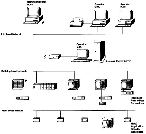
Figure 1.30 The Landis & Gyr BEMS. (Courtesy: Landis & Staefa Ltd.)

1.4 System configuration

At the strategic level, control systems are configured in four stages.

2 Stage 2. Add all measuring and adjusting control devices and identify the signals associated with each device:

3 Stage 3. Prepare a points schedule which lists the total number of control and monitoring I/O points for the system and which can be used to determine the number or required usage of the local outstation or UC. The following should be identified:

4 Stage 4. Specify the logical and functional requirements of the control system which will, in turn, be used for specifying any specialist software requirements and to determine the need for any ASCs as well as for the programming of UCs and outstations. There are four logical/functional outcomes to consider:

The various stages are illustrated in Example 1.1. For a more substantial treatment, see Newman (1994), upon which the following is based. Other work on the planning, configuration and software specification of BEMS can be found in Bynum (1991) and Mumma & Tsai (1991).

Example 1.1

The air handling arrangement of Figure 1.7 is used as an illustrative example of control system configuration.

Figure E1.1.1 Basic system schematic.

Stage 1

Figure El.1.1 shows the basic system schematic – the essential starting point for control system planning. At this point, air flow rates and water flow rates will be known, as will all plant duties (fans, coils and the heat recovery device, HRX).

Stage 2

In Figure El.1.2, all control measuring and positioning devices have been added together with their associated I/O signal types. The numbering system for the resulting ‘points’ is of a form that could be used as practical system addresses. The preceding letters represent the signal type, the first digit signifies a plant reference (1 has been used in this example) and the remaining two digits represent the point reference. Note that the point reference number is incremented in 10s which allows additional points to be added later if needed.

Stage 3

We are now in a position to draw up the points schedule. This is given in Table El.1.1. The points schedule is now used to select the nujnber and disposition of outstations or UCs. We have a need for nine inputs and 10 outputs.

For example, suppose we chose to adopt the Unitron system based on UC16 controllers. The UC16 has eight universal inputs and eight analogue outputs. For the plant considered, we would need two UC16s leaving us with seven spare input points and six spare outputs (the switched voltage binary outputs can be done from the analogue board).

Figure E1.1.2 Control devices and I/O signals.

Stage 4

The following control logic and functionality can now be identified.

c Status – monitoring

d Status – alarm

In this chapter we have taken a fairly broad look at many of the practical HVAC control systems; how they are configured and what, in principle, they seek to achieve. These are actually the routine considerations of HVAC control in practice. Having selected a system and identified what we want it to do the fundamental question remains: Will it work? In the next chapter we will move one step closer to equipping ourselves to answer this question by taking a look at the characteristics and selection procedures for the various components that make up a control system.

References

Akbari, H., Warren, M., Harris, J. (1987) Monitoring and control capabilities of energy management systems in large commercial buildings. ASHRAE Transactions, 91 (1), 961–973.

Atkinson, G.V., Martino, P.E. (1989) Control of semiconductor manufacturing cleanrooms. ASHRAE Transactions, 95 (1), 477–482.

Birtles, A.B. (1985) Selection of Building Management Systems. BRE Information Paper IP 6/85, Building Research Establishment, Garston.

Birtles, A.B., John, R.W., Smith, J.T. (1985) Performance of a PSA Trial Energy Management System. BRE Information Paper IP 2/85, Building Research Establishment, Garston.

Boyens, A., Mitchell, J.W. (1991) Experimental validation of a methodology for determining heating system control strategies. ASHRAE Transactions, 97 (2), 24–35.

Braun, J.E., Klein, S.A., Beckman, W.A., Mitchell, J.W. (1989) Methodologies for optimal control of chilled water systems without storage. ASHRAE Transactions, 95 (1), 652–662.

Bushby, S.T. (1988) Application layer communication protocols for building energy management and control systems. ASHRAE Transactions, 94 (2), 494–510.

Bushby, S.T. (1990a) Testing conformance to energy management and control system communication protocols – Part 1: test architecture. ASHRAE Transactions, 96 (1), 1127–1133.

Bushby, S.T. (1990b) Testing conformance to energy management and control system communication protocols – Part 2: test suite generation. ASHRAE Transactions, 96 (1), 1134–1141.

Bynum, H.D. (1991) Plan and specification documentation of a direct digital control/building management system. ASHRAE Transactions, 97 (1), 773–779.

CIBSE (1985) Applications Manual – Automatic Controls and Their Implications for Systems Design. Chartered Institution of Building Services Engineers, London.

Clark, R.J., Ghandi, T., Hanus, S. (1991) DDC vs. pneumatics: choosing HVAC controls for today’s buildings. Consulting and Specifying Engineer, 9 (8), 84–88.

Clemens, R.B. (1996) Control options for various humidification technologies. ASHRAE Transactions, 102 (2), 607–612.

Cole, J.P., Holness, G.V.R. (1989) Use of programmable controllers for HVAC control and facilities monitoring systems. ASHRAE Transactions, 95 (1), 492–497.

Englander, S.L., Norford, L.K. (1992) Saving fan energy in VAV systems – Part 2: supply fan control for static pressure minimisation using DDC zone feedback. ASHRAE Transactions, 98 (1), 19–32.

Fisk, D.J. (1981) Thermal Control of Buildings. Applied Science, London.

Hartman, T.B. (1990) Employing EMS to test short-term energy effectiveness of control systems. ASHRAE Transactions, 96 (1), 1113–1116.

Hartman, T.B. (1993) Direct Digital Controls far HVAC Systems. McGraw-Hill, New York.

Honda, Y., Inoue, M., Ito, Y., Sato, T. (1993) Integrated network architecture for heating, refrigerating and air conditioning. ASHRAE Transactions, 99 (2), 230–236.

Janu, G.J., Wenger, J.D., Nesler, C.G. (1995) Strategies for outdoor airflow control from a systems perspective. ASHRAE Transactions, 101 (2), 631–643.

Kärki, S.H., Lappalainen, V.E. (1994) A new emulator and a method for using it to evaluate BEMS. ASHRAE Transactions, 100 (1), 1494–1503.

Kelly, G.E., May, W.B., (1990) The concept of an emulator/tester for building energy management system performance evaluation. ASHRAE Transactions, 96 (1), 1117–1126.

Kelly, G.E., May, W.B., Kao, J.Y. (1994) Using emulators to evaluate the performance of building energy management systems. ASHRAE Transactions, 100 (1), 1482–1493.

Kintner-Meyer, M., Emery, A.F. (1995) Optimal control of an HVAC system using cold storage and building thermal capacity. Energy and Buildings, 23, 19–31.

Lewis, M.A. (1990) Microprocessor control of centrifugal chillers – new choices. ASHRAE Transactions, 96 (2), 800–805.

Li, H., Ganesh, C., Munoz, D.R. (1996) Optimal control of duct pressure in HVAC systems. ASHRAE Transactions, 102 (2), 170–174.

Lowry, G. (1996) Survey of building and energy management systems user perceptions. Building Services Engineering Research and Technology, 17 (4), 199–202.

Lute, P.J., van Paassen, D.H.C. (1990) Integrated control system for low energy buildings. ASHRAE Transactions, 96 (2), 889–895.

Mamula, L.J., Cuk, D., Kramer, B. (1989) Microprocessor-based control of a close tolerance temperature industrial building. CLIMA 2000 – Second World Congress on Heating, Ventilation, Refrigeration and Air Conditioning, 338–345.

Mumma, S.A., Tsai, Y.-T. (1991) Direct digital control documentation employing algorithms in matrix format. ASHRAE Transactions, 97 (1), 780–790.

Mutammara, A.W., Hittle, D.C. (1990) Energy effects of various control strategies for variable-air-volume systems. ASHRAE Transactions, 96 (1), 98–102.

Newman, H.M. (1994) Direct Digital Control of Building Systems. John Wiley, New York.

Norford, L.K., Rabi, A. (1987) Energy management systems as diagnostic tools for building managers and energy auditors. ASHRAE Transactions, 93 (2), 2360–2375.

Payne, P.P. (1988) What distributed microcontrollers bring to the building management system. ASHRAE Transactions, 94 (1), 1503–1513.

Peitsman, H.C., Wang, S., Kärki, S.H. et al. (1994) The reproducibility of test on energy management and control systems using building emulators. ASHRAE Transactions, 100 (1), 1455–1464.

Peterson, K.W., Sosoka, J.R. (1990) Control strategies utilising direct digital control. Energy Engineering, 87 (4), 30–35.

Shepherd, K.J., Levermore, G.J., Letherman, K.M., Karayiannis, T.G. (1993) Analysis of VAV networks for design and control. CLIMA 2000 Conference, London.

Smith, R.B. (1990) Importance of flow transmitter selection for return fan control in VAV systems. ASHRAE Transactions, 96 (1), 1218–1223.

Sosoka, J.R., Peterson, K.W. (1988) Building a control system from the bottom up using application-specific controllers. ASHRAE Transactions, 94 (1), 1521–1529.

Tung, D.S.L., Deng, S. (1997) Variable air volume air conditioning system under reduced static pressure control. Building Services Engineering Research and Technology, 18 (2), 77–83.

Visier, J.C., Vaezi-Nejad, H., Jandon, M., Henry, C. (1994) Methodology for assessing the quality of building energy management systems. ASHRAE Transactions, 100 (1), 1474–1481.

Wang, S., Haves, P., Nusgens, P. (1994) Design, construction, and commissioning of building emulators for EMCS applications. ASHRAE Transactions, 100 (1), 1465–1473.

Warren, B.F., Harper, N.C. (1991) Demand controlled ventilation by room C0₂ concentration: a comparison of simulated energy savings in an auditorium space. Energy and Buildings, 17, 87–96.

Wong, A.K.H., James, R.W. (1990) Multiple liquid chillers: intelligent control. Building Services Engineering Research and Technology, 11 (4), 125–128.

Zaheer-uddin, M., Rink, R.E., Gourishankar, V.G. (1990) Heuristic control profiles for integrated boilers. ASHRAE Transactions, 96 (2), 205-211.