7 System identification and controller tuning

7.1 System identification

Much of what we have looked at so far has depended on the ability to build a mathematical representation of a system from first principles using established theory, backed up with a few judicious assumptions. There are of course circumstances in which this is either not necessary (if, for instance, the plant or system exists and it is possible to derive a much more accurate representation of the plant by observing its actual performance) or not possible (the derivation of a mathematical model from first principles is too complex or requires too many questionable assumptions). System identification is the process by which mathematical representations of dynamic systems can be obtained from performance data collected from the actual plant or physically similar plant. This technique is at the heart of adaptive control which we will look at in Chapter 8. Identification applied to HVAC plant has received considerable attention (Penman, 1990; Zaheer-uddin, 1990; So et al., 1995; Coley & Penman, 1992).

The process-reaction curve

This is the simplest method of identification and leads to a transfer function representation of the plant which can subsequently be used to estimate required controller parameters or can be used with any of the modelling, stability and response methods considered in earlier chapters.

Sufficient data to derive a process–reaction curve can be obtained by carrying out a simple test on-site. Any controller present is switched to manual; the system is now under open-loop conditions. The positioning device (e.g. valve or damper actuator) is manually adjusted by a small amount, resulting in an open-loop step response by the system. This response is plotted, forming a process–reaction curve.

A response of the form shown will usually be obtained (Figure 7.1). Note the dead-time component. This is the point at which the response will have cut the time axis were the response of a purely exponential form. In practice, a mathematical model can be easily fitted to the process-reaction curve in the form of a first-order lag plus dead time; this form of representation has been dealt with in a number of places in this book.

The process-reaction curve can therefore be approximated by

where K_p = the overall plant gain, t_d = the apparent system dead time and τ = the overall system time constant. With a step input, we can express the time-domain form as

Figure 7.1 Process-reaction curve.

where Δy = the change in the response variable, y(t) = the response variable value as a function of time, y(0) = the initial response variable value and t = time.

All that remains is to determine values for t_d and τ. To do this, we solve equation (7.2) at two arbitrary points in time. The arbitrary points in time can be anywhere on the response curve above the dead time and below the final value. In most cases, the following arbitrary times will suffice:

Substituting these arbitrary times for t in equation (7.2) leads to

Thus, having plotted the process-reaction curve, we note the values of time corresponding to 28.35% and 63.21% of Δy, the overall change in the response variable, from the curve. We then put these time results into equations (7.3) and (7.4) and solve them for t_d and τ.

Besides using the resulting estimated transfer function with many of the techniques we have explored earlier in this book, t_d and τ form the basis of a variety of controller parameter recommendations, some of which we will look at in section 7.3. Meanwhile, the following example illustrates this simple method of model fitting.

Example 7.1

An open-loop step response test has been conducted on a hot water to air heating coil by manually adjusting the heating control valve by 10% of its range and observing the resulting change in off-coil air temperature. The following results were obtained (given in y(t) format in which y is in °C and t in seconds).

Solution

The open-loop response data are plotted to produce a process-reaction curve (Figure E7.1.1). We note that our two arbitrary times (equations (7.3) and (7.4)) coincide with 28.35% and 63.21% of the overall change in response (i.e. 30.41°C and 30.92°C respectively) at 112 and 273 seconds respectively (t₁ and t₂ in Figure E7.1.1). Substituting these times into the simultaneous equations gives the following:

leading to

Figure E7.1.1 Process-reaction curve.

We are now in a position to fit the model to the data. For fractional changes in heating valve position, u(s), the gain between the off-coil temperature, θ_ao(s), and valve position will be 1.46/0.1 = 14.6. Thus,

This is quite a useful result, for if it were necessary to carry out some further detailed analysis on the system (for example, to investigate in detail various options for improving control), we now have a transfer function representation of the system at our disposal.

Autoregressive models

Several structures exist for the fitting of models to much more detailed experimental data than that considered in the previous section, including the presence of disturbance or noise inputs. A summary of some of the leading methods is given below. A more substantial treatment of the subject can be found in a number of texts – see for example Ljung (1987) or Wellstead and Zarrop (1991). Note that t in the following refers to sampled time.

The autoregressive (AR) structure

The simplest model structure relates a time-series output, y(t), to a noise or disturbance term, e(t), as follows:

where

This forms the autoregressive (AR) model structure, and A is a polynomial in z.

The ARX structure

For closed-loop control, there will be an input, u(t), and the AR model is therefore inappropriate for a full description of the data. Hence an autoregressive with independent or exogenous input (ARX) model structure can be defined:

where

The ARMAX structure

A further refinement for situations in which the disturbance can be meas­ured is to introduce a time-series disturbance parameter which results in the autoregressive moving average with exogenous input structure:

where

The ARIMAX structure

For models which include one or more disturbance inputs, the random nature of many disturbance patterns is not always adequately represented in the ARMAX structure. This situation can be improved by integrating the C time series with respect to time which can be conveniently achieved by introducing the discrete-time integrator 1/(1 – z^–l). The autoregressive integrated moving average with exogenous input (ARIMAX) structure results:

where

Note that the disturbance takes the form of white noise in the special situation where C = A = 1.

Other model structures include the output error (OE) structure, in which the disturbance is treated as white measurement noise and e(t) is regarded as an error with respect to the undisturbed output, and a refinement to this, Box–Jenkins, in which the output error is parametrised (for a full treatment see Ljung, 1987).

Estimation

System identification using any one of the various model structures involves three main stages:

•  Estimate values of the model parameters, A, B, etc.

•  Verify the resulting model using, ideally, data which were not used in model estimation.

In many cases, the nature of any known disturbances will determine the best model structure and it might often be desirable to test the results from a number of different model structures in order to find the best one. For many applications, the ARX model structure will give satisfactory results; indeed the ARX structure tends to be the most commonly used. Verification will therefore determine whether the results obtained from a given model structure are adequate, or whether an alternative model structure should be investigated. It will also enable a choice to be made as to the best combination of parameters in a given model structure.

The routine part of system identification is the estimation of the parameters themselves. In some applications, the input/output (u(t) . . . y(t)) sequence will contain a dead-time delay of nk time samples, so if we consider the case of the ARX structure, the form of model offered is:

Thus the current output, y(t), is related to previous values of output and input, which may include a delay of nk time samples in the input sequence. Note that b₀ will always be zero so that the model will be physically realisable (i.e. based on known previous values) and nk = 1 signifies no dead-time delay between input and output sequences.

Estimation therefore involves the derivation of the parameter set which, since applicable to an evolving time series of input/output values, will be a column vector, ,

By far the most common method of parameter estimation is the least-squares algorithm (for a proof, see Wellstead & Zarrop, 1991),

where

Note that the above assumes that there is no disturbance sequence present (this would merely add a further set of elements to the X matrix after the u(t) sequence).

We also note that

where ê is a vector of modelling errors.

We will now demonstrate the least-squares algorithm in the estimation of a model from some experimental data.

Example 7.2

The data given in Table E7.2.1 relate the room temperature, θ_r(t), to control signal, u(t), for the feedback space heating of a room. The data have been sampled at uniform intervals in time during a morning period (including the preheating period). The data in Table E7.2.2 represent the same observations made one day later. (These data are in fact segments of the more substantial data set used in Example 7.3 and are based on the performance monitoring of a campus building at the University of Northumbria at Newcastle (Hudson & Underwood, 1996).)

Fit a two-input two-output (four-parameter) ARX model with zero dead time to the data recorded on day 1 and verify the resulting model using the data recorded on day 2.

Solution

First, we note that the form of model will be ARX ARX (2, 2, 1) for two input parameters, two output parameters and zero dead-time, i.e.

and b₀ is zero so that the model is feasible (i.e. based entirely on past values). We therefore require estimates of a₁, a₂, b₁ and b₂ from the day 1 data.

The parameter estimate will be,

In most cases involving dynamic data, a more refined model results from fitting to deviations from the data mean values. This also produces a parameter set appropriate to transfer function representation of the model, if required. Removing the mean values from the day 1 data, the values in Table E7.2.3 are obtained.

X can now be formed from the input and output sequences from rows 1–6 and 0–5 in Table E7.2.3, representing parameter estimate bases for θ_r(t – 1), θ_r(t – 2) and u(t – 1), u(t – 2) respectively. Thus X will be a matrix of four columns and six rows,

and the transpose of X will be

With some effort, we now obtain

The output, y, will be a column vector formed from the values θ_r(2 . . . 7) i.e.

and therefore

The parameter estimate, , is now given by

We can now express our model, remembering that θr(t) and u(t) are expressed as deviations from their mean values,

Note that the matrix algebra above could be handled with the following MATLAB operations (MATLAB, 1996). Given the matrix X, to obtain the transpose,

For the inverse of X^TX,

Note also that the time-domain model form of equation (E7.2.3) can be expressed in the form of a discrete-time transfer function, G_r(z),

We can now apply the estimated model (equation (E7.2.3)) to the verification data from the day 2 measurements in order to establish how adequate our model is. The results are shown in Table E7.2.4. Evidently, modelling error is initially quite high due to the lack of initial model results at t = 1, –2 from which to construct model predictions at t = 0, 1. Nevertheless, the error does recede and a reasonable mean error across the six-sample prediction of 0.38K is obtained.

Manual autoregressive model fitting of this type, even to small groups of data such as that considered in this example, is likely to prove intractable in practice without the help of computational methods. Example 7.3 illustrates the potential of autoregressive identification for a much more substantial family of data using such methods.

Figure E7.3.1 Heating system monitored data.

Example 7.3

Hudson has monitored the space air temperature and control valve signal in a number of zones of a heated and naturally ventilated campus building at the University of Northumbria at Newcastle (Hudson & Underwood, 1996). Figure E7.3.1 gives a five-day (Monday to Friday) sample of the data for a typical zone from December 1995. The data were recorded at 15 min intervals. The heating system consists of a feedback loop using a thermistor in the space, with a control signal generated from a building management system PID control algorithm which sampled at 5s intervals and was tuned with a gain of 0.1K^–1, integral action time of 10min and derivative action time of 5min.

From a control point of view, we can identify some interesting features in these data. Each day commences with the heating system preheating at full capacity – note the protracted preheating on the first day (Monday), following the weekend shutdown. From mid-morning (mid-day in the case of the Monday cycle), the heating reverts to modulating control and there is clear evidence of low-frequency oscillatory behaviour during these periods of modulating control.

Model fitting

A four-parameter ARX model (with zero dead time) has been fitted to the data using the MATLAB system identification toolbox (Ljung, 1988) – indeed most statistical or spread-sheet programs offering autoregressive modelling functions could be used for this. The procedure adopted is as follows:

A ‘best-fit’ model was found to be an ARX(4, 6, 1), which had a mean fitting error of 0.00267. However, a good fit was also obtained with the following ARX(2, 2, 1) structure (mean fitting error 0.00305):

and thus

Evidently, the estimated parameters here are quite different to those obtained from the much smaller segment of data used in the previous example (equation (E7.2.3)). This is not to say that the above model is better; merely that it reflects a more substantial set of observations.

Figure E7.3.2 shows how the model-predicted room temperature compares with the second segment of measured values. Certainly, the middle days reproduce quite well but the first day predictions are not good. Once again, this is due to the need to set initial predicted values of zero (i.e. the first pair of input/output values used to get the model started are not known). The error associated with this can be appreciated from Figure E7.3.3 in which the first pair of values from the measured data set are used for the first predictions of the model (this is of course technically cheating, because these values are not known to the model). Clearly then, there will always tend to be a certain amount of front-loaded error in identified models of this type.

Figure E7.3.2 ARX(2, 2, 1) model performance.

Figure E7.3.3 ARX(2, 2, 1) model performance with modified initial values.

Though two models were identified (ARX(4, 6, 1) and ARX(2, 2, 1)), Figure E7.3.4 shows that there is little to choose between them; and the four-parameter model is simpler.

One final point: there are two dominant frequencies in these data. One is due to the daily system switching pattern whilst the other is due to system dynamics. It will of course be difficult to fit a model with excellent robustness in terms of reproducing all features of such a complex pattern of data. One possible remedy where a higher-quality model is needed would be to identify separately the daytime data only. Figure E7.3.5 shows the performance of an ARX(2, 1, 2) fitted to a segment of daytime data only for one of the daily patterns forming Figure E7.3.1. Again, a ‘best fit’ was found to be an ARX(2, 6, 1) but an ARX(2, 1, 2) gave results which were almost as good. This ARX(2, 1, 2) for this confined data set is as follows:

Figure E7.3.4 ARX(2, 2, 1) and ARX(4, 6, 1) model comparison.

Figure E7.3.5 ARX(2, 1, 2) model fitted to daytime cyclic data only.

a₂ = –0.6119,

b₁ = 0.0046

and thus

Figure E7.3.5 shows that the cyclic pattern of activity is much better represented by this model, even though the model does not represent the peaks and troughs especially well. In many cases then, the best resort will often be to fit a combination of models, especially where a multi-modal pattern of data is evident.

Autoregressive system identification is a straightforward enough business provided that suitable computational tools are available though the quality of model fit can vary considerably. In Chapter 9 we will discuss the use of artificial neural networks for identification and will see that these have the potential to produce excellent representations of complex data patterns. We will also return to a more practical application of ARX methods a little later in Chapter 8.

7.2 Assessing the quality of response

Stable operation is the primary concern in control system design. However, once stable operation has been established, further adjustment will lead to the ‘optimum’ response of a plant as judged by a number of performance quality criteria. We will consider some of the basic response quality criteria in the following then go on to see how we might achieve them with reference to controller tuning.

Synoptic criteria

In the response of Figure 7.2, we can identify a number of features which constitute measures of how well a plant is behaving under control. The figure shows the response of a feedback control system to a unit change in set point. When tuning a controller, minimising the following response features will lead to some kind of an ‘optimum’ dynamic response.

There are some response features which do not necessarily require to be minimised, but adjusted to within some specified tolerance. The percentage overshoot, (a/r) × 100 (where r is the target response required), and the decay ratio, a/b, give indications of the degree of damping present. A common ‘rule of thumb’ for process control is to target a decay ratio of about one-quarter.

Error-integral criteria

Lopez et al. (1967) propose error-integral criteria as a more rigorous way of evaluating the quality of response of a control system. These criteria are more difficult to evaluate than synoptic methods, other than in on-line situations. There are several ways of applying error-integral criteria but all are based on the time integral of the error experienced by a control system following some predefined disturbance (usually a small step change in set point).

Figure 7.2 Synoptic response quality criteria.

Consider the typical set point response of Figure 7.3. The area of the hatched regions represents the integral of the error with respect to time. Discriminating between positive contributions to error (above the desired response value) and negative contributions (below the desired response) is unnecessary so we can define an integral of absolute error (I_(|ε|)),

Clearly, a perfect response is satisfied at I_(|ε|) = 0, but this will never be achievable in practice due to intrinsic system dynamics. Instead, a ‘good’ response is obtained by minimising I_(|ε|) in some way.

For conventional stand-alone controllers with fixed settings, this minimising procedure will be a matter of hands-on trial and error, but for programmable controllers it should be possible to use this criterion as a basis for on-line controller parameter adjustment. Nominally fixed-parameter self-tuning controllers work in this way (for examples, see Kamimura et al., 1994; Underwood, 1989; Nesler, 1986; Pinnella et al., 1986) – note that automated tuners of these types should not be confused with adaptive controllers which we consider in Chapter 8.

In some circumstances, it may be desirable to weight the integral error in some way. The integral of error squared (I_(ε²)) ensures that large values of error contribute more heavily to the integral than smaller values, Large error tends to occur early in a response, immediately following some disturbance, and take the form of overshoot/undershoot. Hence, minimising this criterion will tend to result in minimised oscillation in a response.

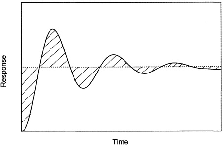
Figure 7.3 Integral-error criteria.

Another possibility is the integral of time multiplied by absolute error (I_(|ε|t)),

Because time accumulates independently after a disturbance, this criterion weights more heavily errors that occur late in time (such as offset), putting less emphasis on errors which occur immediately after the disturbance (i.e. overshoot).

7.3 Fixed-parameter controller tuning methods

The process of adjusting a control system or control loop to achieve its best response characteristics is often referred to as tuning the control loop. Essentially, this is the process of commissioning and optimisation of system performance. Once a system has been installed, then the tuning process involves adjusting the various controller parameters or settings in order to achieve the best possible response (such as a minimum error-integral value). In traditional fixed-parameter control systems, this is usually achieved not by scientific reasoning but by trial and error – backed up by some initial intelligent guess work, though some work has been done on systematic methods for obtaining optimum controller parameters (see for example Kelly et al., 1991). We will look at this later but first we need to consider what degrees of freedom we have in the pre-commissioned system.

Controller parameters

The 1980s saw a dramatic shift in the UK from the use of electronic and pneumatic analogue control systems for HVAC applications, to digital control systems and, with it, the expansion of distributed control and building management systems.

Overwhelmingly, the HVAC control algorithm in use in these systems is the discretised form of the three-term proportional-integral-derivative (PID) controller. We looked at this in Chapter 5 (section 5.5) and the equations are reproduced below in sampled time form:

where u(n) and e(n) are the control signal and control error at the nth sampling instant, respectively, u(n – 1) and ε(n – 1) are the control signal and error at the previous sampling instant, ε(n – 2) is the control error at the previous but one sampling instant, and the coefficients are

Thus control system ‘degrees of freedom’ are the parameters: K_c = the controller gain, i_t = the integral time (or reset time), d_t = the derivative time (or rate time) and T = the sampling time interval.

Equation (7.18) is therefore used to calculate the required control signal at time, t = nT, from previous values of control signal and control error. Practical algorithms take this form though there are some minor variations. For example, some make the feedback variable value the object of the derivative action instead of control error. Integral and derivative parameters are sometimes expressed as an integral gain K_c/i_t and a derivative gain K_cd_t, respectively.

There may also need to be a provision for integral wind-up. Wind-up occurs when, during a protracted period in which the error is high, the control signal saturates (i.e. settles at its maximum value) due to the accumulated integral. A sustained period of negative error would be needed to cause a reduction in the control signal. Instead, a mechanism can be included in the algorithm to reset the saturated signal rapidly.

Note that setting i_t = ∞ and d_t= 0 effectively eliminates any integral and derivative control action, leaving us with purely proportional control.

We will come back to these parameters in a later section but first let us look at two other aspects of controller set-up.

Proportional band and proportional gain

For largely historical reasons, many of the controllers and control algorithms used in HVAC applications use a proportional band setting as opposed to proportional gain, though it appears that this term is gradually being replaced by the latter.

The proportional band, p, is defined as the range of the controlled variable to which the control signal is directly proportional. It can be expressed simply as a band of the controlled variable value. As a controller setting, the proportional band is usually expressed as a percentage of the corresponding overall range of the system,

where δy represents the band of the controlled variable within which control is to be maintained and Δy is the maximum range of the controlled variable which is determined by the limits of the capacity of the plant. Thus, the percentage proportional band is also sometimes called the throttling range (CIBSE, 1985).

The following example illustrates the relationship between the proportional band and gain.

Example 7.4

A proportional fan speed controller is used to maintain a critical static pressure in a space. The fan when operating at top speed can maintain a static pressure of 300Nm^–2 in the space, and at its minimum speed, the static pressure will be 25Nm^–2. The speed controller has been set up to achieve a proportional band of ±10Nm^–2. What is the gain and percentage proportional band of the controller?

Solution

The proportional band in units of the controlled variable is, therefore, 10 – ( – 10) = 20Nm^–2. The gain of this controller will therefore be

and the percentage proportional band will be

Now suppose that the controller proportional band setting is adjusted to 15%. The range (or proportional band) of the control variable will be

and the modified gain will be

Note that the proportional band and proportional gain settings of a controller are inversely related.

Identifying PID terms

In many applications, there will be no advantage in adopting the derivative term in a PID controller; in fact, the PI controller is quite common in HVAC applications, and in a number of these cases, purely proportional control might suffice with adequate results. The reasoning is as follows. If the system has sufficient intrinsic stability to allow a purely proportional controller to be used with a high gain (i.e. low proportional band) without fear of instability, then as we know from section 4.1 the high gain setting will be reasonably free from offset and satisfactory control will result. If the high gain is not possible due to the danger of an unstable response, then a low-gain integral PI controller will be necessary and it becomes necessary to fix a sufficiently low value of integral time to eliminate the offset. This then prompts the need for derivative action to compensate for the resulting slowness of response caused by the integral action; full PID control is necessary.

Though most current generation controllers will offer full PID control, there are clearly advantages in set-up time if the necessary combination of controller term (s) is known prior to commissioning. Borresen (1990) has proposed a simple method which is summarised below.

Using an open-loop process-reaction test, the system gain, Kp, and time constant and dead time (τ, t_d), are obtained (see section 7.1). Borresen argues that the controllability of a system depends on the system gain, offset, and the ratio of the dead time to time constant of the system. He defines the relative control difficulty, DREL, as

where Δy_ss is the required maximum offset (equation (7.23) implies that there must be some tolerance to offset, even after applying integral control action).

The interpretation of DREL is summarised in Table 7.1. We note that DREL = 1 when the offset is equal to the proportional band and it would therefore be unnecessary to specify other than simple proportional control. At DREL > 1, offset becomes a problem and integral action becomes necessary. The introduction of derivative action at the higher DREL can be thought of as compensation for system dead-time effects.

Example 7.5

For the system parameters determined in Example 7.1, find the relative control difficulty and, hence, determine which of the three term control actions should be specified. The control system should operate within a maximum offset of 1.0K.

Solution

We use the system time constant and dead-time characteristics in equation (7.23) to determine the relative control difficulty, noting that the maximum acceptable offset is to be 1.0K:

From this, we conclude that the system will experience ‘medium control difficulty’ (Table 7.1), since DREL > 1. We therefore specify a PI controller.

Methods of establishing controller parameters

There are several methods for establishing the required controller parameters or settings to achieve the ‘best’ control for a given control system. With conventional fixed-parameter controllers, these parameters can often only be determined by trial and error. The methods we will look at in the following can be used to establish ‘first guess’ approximations to inform this trial-and-error process.

We noted that there are up to four controller parameters for traditional P, PI or PID control, giving up to four degrees of freedom for system tuning. These are the sampling interval, T, and up to three controller settings. We will look at the latter in the following sections, but it is appropriate to reflect once more on the sampling interval, which we first considered in section 5.4.

For a system which can be adequately described by a first-order lag plus a dead-time term, we note from section 3.5 that the dead-time term can be treated in exactly the same way as a transport lag and can be represented by a Padé approximation. This results in our simple lag plus dead-time model having two poles and a zero in the right half of the s-plane; thus the dominant pole is the inverse of the time constant. One of the ‘rules of thumb’ discussed in section 5.4 was to fix T (as a maximum) of one-tenth of the dominant time constant. Therefore, Example 7.1 under propor­tional control might be expected to operate satisfactorily with a sampling interval of about 24s. We also noted in Chapter 5 (Example 5.5) that with the sampling interval low enough, our system might be expected to behave like a continuous-time system but with a need for a lower propor­tional gain and, as a consequence, a tendency for offset which must be checked using integral control. On the other hand, a high sampling inter­val tends to result in a response which resembles a continuous system with high dead time, a combination which equation (7.23) confirms will lead to reduced stability.

In summary for the sampling interval, unless we expect high-frequency disturbances (i.e. rapid load disturbances or measurement noise, not common in HVAC applications), a very low sampling interval is desirable. Proportional control alone is unlikely to be adequate in most cases. In any event, the sampling interval should be less than any dead time and within one-tenth of the dominant time constant if known.

Ziegler and Nichols tuning based on closed-loop criteria

The earliest work on controller tuning with particular reference to process control was due to Ziegler & Nichols (1942). In the first of two methods, the controller participates in the loop (i.e. the control system is maintained in its closed-loop mode) and the controller is set for proportional control only. The controller gain is gradually increased (i.e. proportional band decreased) as small step disturbances are introduced until a point is reached where the control loop is marginally stable. At this point, the controlled variable will be seen to oscillate at uniform amplitude (Figure 7.4).

The following characteristics at marginal stability are noted: K’_c, the controller gain at marginal stability; and p_w, the period of oscillation at marginal stability. From these, settings can be estimated using the expressions given in Table 7.2. These estimates are based on achieving one-quarter decay ratio to a step change in input to the controller.

This method is very simple to carry out under site conditions. However, there are two disadvantages which restrict its use:

Figure 7.4 Closed-loop response at marginal stability.

Table 7.2 Ziegler and Nichols tuning estimates - closed-loop criteria (Ziegler & Nichols, 1942)

Tuning based on open-loop response criteria

To overcome the disadvantages imposed by extracting the closed-loop data, alternative estimates for controller settings have evolved based on the identified parameters, τ and t_d, from the open-loop process-reaction curve (section 7.1).

Ziegler and Nichols estimates As well as the work they did based on closed-loop performance characteristics, Ziegler & Nichols (1942) also offer an estimate based on open-loop process–reaction curve information, again based on the one-quarter decay ratio criterion (Table 7.3).

These classical parameter estimates have been used widely in process control for many years, though Geng & Geary (1993) found that they can lead to conservative results when used in some HVAC applications and propose a modified procedure.

Cohen and Coon settings Cohen & Coon (1953) pointed out that the Ziegler & Nichols (1942) work did not consider system ‘self-regulation’ resulting from dead-time effects and they derived alternative setting estimates based on the open-loop process reaction curve data. These are summarised in Table 7.4.

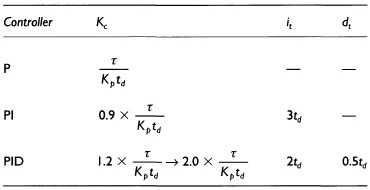
Lopez et al. estimates Lopez et al. (1967) make recommendations for estimating controller settings which seek to minimise the various error-integral criteria (see section 7.2). They also make recommendations for achieving either good set point response or good disturbance-rejection response. The following summarises their recommendations for disturbance rejection control:

The constants, a–f, are given in Table 7.5.

One of the main advantages of the open-loop process-reaction curve methods is that they allow a simple identified model to be fitted to the system. This, in turn, enables a much wider analysis to be carried out on an existing system if required, using, for example, simulation methods. The following example compares the results of the various methods.

Example 7.6

Using the results of Examples 7.1 and 7.5, select and compare suitable controller parameters using the various methods discussed in this section.

Solution

From Example 7.5, we recall that a PI controller should be used for this case.

• Ziegler and Nichols estimates

Based on the open-loop process-reaction curve of Example 7.1, we note that the plant gain, K_p, is 14.6K^–1 and the dead time and time constant are 31.5s and 241.5s respectively. Referring to Table 7.3 for a PI controller,

and

As a matter of interest, it is also possible to find the setting estimates based on Ziegler and Nichols’ closed-loop performance criteria. We note from Example 7.1 that the closed-loop model for this system is

Using a Routh array based on the characteristic equation of the above, we can obtain the controller gain and period of the response based on the system natural frequency, ω_n, as described in Example 4.2 (Chapter 4). The results are K'_c = 1.119 and p_ω = 93.1.

Referring to the estimates of Table 7.2, the alternative Ziegler and Nichols tuning estimates will therefore be

and

• Cohen and Coon estimates

Based on Table 7.4,

and

• Lopez et al. estimates

We refer to equations (7.24) and (7.25) and the associated constants in Table 7.5. For the absolute error-integral criterion:

and

Similarly, for the squared error-integral criterion:

and

For the time multiplied by error-integral criterion:

and

Table E7.6.1 summarises the various results. We see that most of the estimates are in reasonably close agreement, but we can pick out two of the Lopez et al. results for closer examination since they stand apart from the other results – specifically those estimates based on squared error integral (I_(ε²)) and time multiplied by error integral (I_(|ε|t)). We note that the latter fixes a lower integral time evidently to force the offset (i.e. long-term error) to zero, but in doing so, a lower gain is necessary for stability. The opposite pattern is evident for the squared error-integral criterion.

We should note a particularly important point about the estimates in Example 7.6; they are entirely based on the performance optimisation of a continuous-time process system though we are aware that most modern control is conducted in discrete time. How will these estimates behave when applied to the equivalent discrete-time system when the sampling-time degree of freedom is also introduced? We shall consider this for the two Lopez et al. estimates in a simulation in Example 7.7.

Example 7.7

For the system described by the model of Example 7.1, apply the Lopez et al. controller setting estimates based on (I_(ε²)) and (I_(|ε|t)) to the discrete-time control case with the initial sampling interval taken to be one-tenth of the dominant time constant of the system.

Compare the resulting unit step time response simulations of the continuous-time and discrete-time cases.

Solution

The sampling interval will be 24.15s (one-tenth of the system time constant which in this case is essentially the dominant time constant).

Firstly, we need to discretise the continuous-time system model. If we assume a zero-order hold, then the modified z-transform of equation (5.14) (section 5.3) can be used. Representing the case in which the dead time is a non-integer multiple of sampling intervals (i.e. t_d = (315/24.15) × T = 1.304T), equation (5.14) gives

where A = T/τ, B = (T/τ) × (1 – λ), t_d = 1.304T, λ = 0.304, m = 1 – λ = 0.696, i = 1, K_p = 14.6 and τ = 241.5. We can therefore express the discrete-time form of system model with zero-order hold as

Now we consider the controller. For a PI controller, we recall the discrete-time (z-domain) form as follows (see section 5.5):

where

and b = K_c

For the first of the two Lopez et al. controller settings estimates, K_c = 0.430K^–1 and i_t = 89.7s imply

and b = 0.430

Therefore the discrete-time controller transfer function will be:

and, similarly, for the other,

A comparative simulation model which generates side-by-side results for the discrete-time and continuous-time cases is now generated using a Simulink model (Simulink, 1996). The model is shown in Figure E7.7.1 for the first of the two estimated controllers considered above and is based on a unit step change in set point.

Results

Simulation results from the continuous-time system confirm good responses for either set of settings estimates (Figure E7.7.2). In particular, the I_(|ε|t) criterion has resulted in settings which give minimal oscillation and (slightly) faster settling time than for the I_(ε²)-based estimates.

Figure E7.7.1 Simulink model of discrete- and continuous-time systems.

Figure E7.7.2 Results for the continuous-time case.

However, the discrete-time equivalent system at the second of the two controller settings estimates exhibits instability (Figure E7.7.3) and for the first of the two settings estimates the discrete-time plant was found to show considerable oscillation prior to settling (not shown).

Clearly we must either conclude for this example that the settings estimates, whilst satisfactory for a continuous-time situation, are inadequate for the discrete-time case; or that the one-tenth dominant time constant sampling interval for the latter is unsound when using these settings estimates.

If we modify the settings estimates and leave the sampling interval as it was, our choices are confined to reducing the gain or increasing the integral time or both. In any event, this is likely to lead to offset and protracted response times (as we found in Example 5.5, Chapter 5). The correct option therefore appears to be a decrease in the sampling interval. Indeed decreasing the sampling interval, at least for systems which are free of high-frequency disturbances, leads to the discrete-time system approaching a response which is closer to the equivalent continuous-time system.

 Figure E7.7.3 Discrete-time case (T = 24.15s and I_(|ε|t)-based estimates.

It is possible to show that, with a sampling interval of one-twentieth of the dominant time constant (T = 12.0575s), the discrete-time system continues to give an unstable response for the I_(ε²)-based estimates though a satisfactory response is achieved for the I_(|ε|t)-based estimates.

At a sampling interval of one-fortieth of the dominant time constant (T = 6.0375s), the system and controller transfer functions become

and

Figure E7.7.4 shows that stable offset-free control can now be expected for either set of settings estimates.

Clearly then, for systems which exhibit significant dead time at least, the various settings estimates considered in this section will work, but only when care is taken over the choice of sampling interval, T. It seems clear that the one-tenth time constant ‘rule of thumb’ for T will be too irresolute. Indeed, as a general rule, provided that care is taken with regard to the information loss effect (see section 5.4), it might be concluded for HVAC control that a choice of T as low as is practicable will usually be the best course of action.

Figure E7.7.4 Discrete-time case at T = τ/40.

In this chapter, we have given extensive consideration to the estimation of controller parameters and a reasonable amount of work has been done in this field of relevance to HVAC applications. Bekker et al. (1991) look at the use of a pole–zero cancellation tuning method (pole–zero cancellation is applied to adaptive controller design in Chapter 8). Kasahara et al. (1997) introduce a two-degrees-of-freedom controller which acts separately on feedback and reference signals and go on to propose a tuning method for this, whilst Nesler & Stoecker (1984) evaluate PI settings for HVAC plant experimentally. Pinnella et al. (1986) describe the development of a self-tuning algorithm for a fixed-parameter purely integral controller. A first-order plus dead-time model is fitted to open-loop step response data collected on-line and the results are used to identify an integral gain using Ziegler–Nichols tuning rules. The method is tested on a fan speed regulator and a steam heat exchanger having fast- and slow-response dynamics respectively. Both systems exhibited critically damped responses. Ho (1993) develops a search algorithm for the optimised selection of fixed PID controller parameters. The search uses energy consumption as the objective function as well as a stability criterion. However, the search times are protracted (it is debatable whether the method could be used on-line) and though results seem good, they are compared with simulated reference results only.

Another important aspect of controller performance is performance and fault detection in use – aspects which are beyond the scope of this book. However, several workers have developed methods of fault detection in control systems – see for instance Pape et al. (1991), Solberg & Teeters (1992) or Fasolo & Seborg (1995).

Increasingly, the advantages of adaptive control in which controller parameters are adjusted on-line to accommodate changing circumstances and operating conditions by the plant are being realised. We will therefore give special consideration to this in the next chapter.

References

Bekker, J.E., Meckl, P.H., Hittle, D.C. (1991) A tuning method for first-order processes with PI controllers. ASHRAE Transactions, 97 (2), 19–23.

Borresen, B.A. (1990) Controllability: back to basics. ASHRAE Transactions, 14 (1), 817–819.

CIBSE (1985) Automatic Controls and Their Implications for System Design. Chartered Institution of Building Services Engineers, London.

Cohen, G.H., Coon, G.A. (1953) Theoretical considerations of retarded control. Transactions of the American Society of Mechanical Engineers, 75, 827–834.

Coley, D.A., Penman, J.M. (1992) Second order system identification in the thermal response of real buildings. Paper II: Recursive formulation for on-line building energy management and control. Building and Environment, 27 (3), 269–277.

Fasolo, P.S., Seborg, D.E. (1995) Monitoring and fault detection for an HVAC control system. ASHRAE Transactions, 1 (3), 177–193.

Geng, G., Geary, G.M. (1993) On performance and tuning of PID controllers in HVAC systems. Proceedings of the Second IEEE Conference on Control Applications, Vancouver, 819–824.

Ho, W.F. (1993) Development and evaluation of a software package for self-tuning of three-term DDC controllers. ASHRAE Transactions, 99 (1), 529–534.

Hudson, G., Underwood, C.P. (1996) Effect on energy usage of over-capacity and emission characteristics in the space heating of buildings with high thermal capacity. Proceedings of the CIBSE National Conference, Harrogate.

Kamimura, K., Yamada, A., Matsuba, T., Kimbara, A., Kurosu, S., Kasahara, M. (1994) CAT (computer-aided tuning) software for PID controllers. ASHRAE Transactions, 100 (1), 180–190.

Kasahara, M., Matsuba, T., Murasawa, I., Hashimoto, Y., Kamimura, K., Kimbara, A., Kurosu, S. (1997) A tuning method of two degrees of freedom PID controller. ASHRAE Transactions, 103 (1), 278–289.

Kelly, G.E., Park, C., Barnett, J.P. (1991) Using emulators/testers for commissioning EMCS software, operator training, algorithm development, and tuning local control loops. ASHRAE Transactions, 97 (1), 669–678.

Ljung, L. (1987) System Identification: Theory for the User. Prentice-Hall, Englewood Cliffs, NJ.

Ljung, L. (1988) System Identification Toolbox for Use with MATLAB. The Mathworks Inc., Natick, MA.

Lopez, A.M., Miller, J.A., Smith, C.L., Murrill, P.W. (1967) Tuning controllers with error-integral criteria. Instrumentation Technology, 14 (11), 57–62.

MATLAB (1996) MATLAB The Language of Technical Computing. The Mathworks Inc., Natick, MA.

Nesler, C.G. (1986) Automated controller tuning for HVAC applications. ASHRAE Transactions, 92 (2B), 189–201.

Nesler, C.G., Stoecker, W.F. (1984) Selecting the proportional and integral constants in the direct digital control of discharge air temperature. ASHRAE Transactions, 90 (2B), 834–845.

Pape, F.L.F., Mitchell, J.W., Beckman, W.A. (1991) Optimal control and fault detection in heating, ventilating and air conditioning systems. ASHRAE Transactions, 97 (1), 729–736.

Penman, J.M. (1990) Second order system identification in the thermal response of a working school. Building and Environment, 25 (2), 105–110.

Pinnella, M.J., Wechselberger, E., Hittle, D.C., Pedersen, C.O. (1986) Self-tuning digital integral control. ASHRAE Transactions, 92 (2B), 202–210.

Simulink (1996) SIMULINK 2 Dynamic System Simulation far MATLAB. The Mathworks Inc., Natick, MA.

So, A.T.P., Chan, W.L., Chow, T.T., Tse, W.L. (1995) New HVAC control by system identification. ASHRAE Transactions, 30 (3), 349–357.

Solberg, D.P.W., Teeters, M.D. (1992) Specification of spreadsheet trend log sheets for DDC/EMCS and HVAC system commissioning, energy monitoring, life safety cycles, and performance based service contracts. ASHRAE Transactions, 98 (2), 553–571.

Underwood, D.M. (1989) Response of self-tuning single loop digital controllers to a computer simulated heating coil. ASHRAE Transactions, 95 (2), 424–430.

Wellstead, P.E., Zarrop, M.B. (1991) Self-tuning Systems: Control and Signal Processing John Wiley, Chichester.

Zaheer-uddin, M. (1990) Combined energy balance and recursive least squares method for the identification of system parameters. ASHRAE Transactions, 96 (2), 239–244.

Ziegler, J.G., Nichols, N.B. (1942) Optimum settings for automatic controllers. Transactions of the American Society of Mechanical Engineers, 64, 759–768.