11

Sorting

Sorting means reorganizing data in such a way that it is in ascending or descending order. Sorting is one of the most important algorithms in computer science and is widely used in database-related algorithms. For several applications, if the data is sorted, it can efficiently be retrieved, for example, if it is a collection of names, telephone numbers, or items on a simple to-do list.

In this chapter, we’ll study some of the most important and popular sorting techniques, including the following:

• Bubble sort
• Insertion sort
• Selection sort
• Quicksort
• Timsort

Technical requirements

All source code used to explain the concepts of this chapter is provided in the GitHub repository at the following link:

https://github.com/PacktPublishing/Hands-On-Data-Structures-and-Algorithms-with-Python-Third-Edition/tree/main/Chapter11

Sorting algorithms

Sorting means arranging all the items in a list in ascending or descending order. We can compare different sorting algorithms by how much time and memory space is required to use them.

The time taken by an algorithm changes depending on the input size. Moreover, some algorithms are relatively easy to implement, but may perform poorly with respect to time and space complexity, whereas other algorithms are slightly more complex to implement, but can perform well when sorting longer lists of data. One of the sorting algorithm, merge sort, we have already discussed in Chapter 3, Algorithm Design Techniques and Strategies. We will discuss several more sorting algorithms one by one in detail along with their implementation details, starting with the bubble sort algorithm.

Bubble sort algorithms

The idea behind the bubble sort algorithm is very simple. Given an unordered list, we compare adjacent elements in the list, and after each comparison, we place them in the right order according to their values. So, we swap the adjacent items if they are not in the correct order. This process is repeated n-1 times for a list of n items.

In each iteration, the largest element of the list is moved to the end of the list. After the second iteration, the second largest element will be placed at the second-to-last position in the list. The same process is repeated until the list is sorted.

Let’s take a list with only two elements, {5, 2}, to understand the concept of bubble sort, as shown in Figure 11.1:

Figure 11.1: Example of bubble sort

To sort this list of two elements, first, we compare 5 and 2; since 5 is greater than 2, it means they are not in the correct order, so we swap these values to put them in the correct order. To swap these two numbers, first, we move the element stored at index 0 in a temporary variable (step 1 of Figure 11.2), then the element stored at index 1 is copied to index 0 (step 2 of Figure 11.2), and finally the first element stored in the temporary variable is stored back at index 1 (step 3 of Figure 11.2). So, first, element 5 is copied to a temporary variable, temp. Then, element 2 is moved to index 0. Finally, 5 is moved from temp to index 1. The list will now contain the elements as [2, 5]:

Figure 11.2: Swapping of two elements in bubble sort

The following code will swap the elements of unordered_list[0] with unordered_list[1] if they are not in the right order:

unordered_list = [5, 2]
temp = unordered_list[0]
unordered_list[0] = unordered_list[1]
unordered_list[1] = temp
print(unordered_list)

The output of the above code is:

[2, 5]

Now that we have been able to swap a two-element array, it should be simple to use this same idea to sort a whole list using bubble sort.

Let’s consider another example to understand the working of the bubble sort algorithm and sort an unordered list of six elements, such as {45, 23, 87, 12, 32, 4}. In the first iteration, we start comparing the first two elements, 45 and 23, and we swap them, as 45 should be placed after 23. Then, we compare the next adjacent values, 45 and 87, to see whether they are in the correct order. As 87 is a higher value than 45, we do not need to swap them. We swap two elements if they are not in the correct order.

We can see, in Figure 11.3, that after the first iteration of the bubble sort, the largest element, 87, is placed in the last position of the list:

Figure 11.3: Steps of the first iteration to sort an example array using bubble sort

After the first iteration, we just need to arrange the remaining (n-1) elements; we repeat the same process by comparing the adjacent elements for the remaining five elements. After the second iteration, the second largest element, 45, is placed at the second-to-last position in the list, as shown in Figure 11.4:

Figure 11.4: Steps of the second iteration to sort an example array using bubble sort

Next, we have to compare the remaining (n-2) elements to arrange them as shown in Figure 11.5:

Figure 11.5: Steps of the third iteration to sort an example array using bubble sort

Similarly, we compare the remaining elements to sort them, as well, as shown in Figure 11.6:

Figure 11.6: Steps of the fourth iteration to sort an example array using bubble sort

Finally, for the last two remaining elements, we place them in the correct order to obtain the final sorted list, as shown in Figure 11.7:

Figure 11.7: Steps of the fifth iteration to sort an example array using bubble sort

The complete Python code of the bubble sort algorithm is shown below, and afterward, each step is explained in detail:

def bubble_sort(unordered_list):
    iteration_number = len(unordered_list)-1
    for i in range(iteration_number,0,-1):
        for j in range(i):
            if unordered_list[j] > unordered_list[j+1]:
                temp = unordered_list[j]
                unordered_list[j] = unordered_list[j+1]
                unordered_list[j+1] = temp

Bubble sort is implemented using a double-nested loop, wherein one loop is inside another loop. In bubble sort, the inner loop repeatedly compares and swaps the adjacent elements in each iteration for a given list, and the outer loop keeps track of how many times the inner loop should be repeated.

Firstly, in the above code, we compute how many times the loop should run to complete all swaps; this is equal to the length of the list minus 1 and could be written as iteration_number = len(unordered_list)-1. Here, the len function will give the length of the list. We subtract 1 because it gives us exactly the maximum number of iterations to run. The outer loop ensures this and executes for one minus the size of the list.

Further, in the above code, for each iteration, in the inner loop, we compare the adjacent elements using the if statement, and we check if the adjacent elements are in the correct order or not. For the first iteration, the inner loop should run for n times, for the second iteration, the inner loop should run n-1 times, and so on. For example, to sort a list of three numbers say [3, 2, 1], the inner loop runs two times, and we need to swap the elements a maximum of two times as shown in Figure 11.8:

Figure 11.8: Number of swaps in iteration 1 for an example list [3, 2, 1]

Further, after the first iteration, in the second iteration, we execute the inner loop once as shown in Figure 11.9:

Figure 11.9: Number of swaps in iteration 2 for an example list [3, 2, 1]

The following code snippet can be used to deploy the bubble sort algorithm:

my_list = [4,3,2,1]
bubble_sort(my_list)
print(my_list)
 
my_list = [1,12,3,4]
bubble_sort(my_list)
print(my_list)

The output is as follows:

[1, 2, 3, 4]
[1, 3, 4, 12]

In the worst case, the number of comparisons required in the first iteration will be (n-1), in the second, the number of comparisons will be (n-2), and in the third iteration it will be (n-3), and so on. Therefore, the total number of comparisons required in the bubble sort will be as follows:

(n-1) + (n-2) + (n-3) +.....+ 1 = n(n-1)/2
n(n+1)/2
O(n2)

The bubble sort algorithm is not an efficient sorting algorithm, as it provides a worst-case runtime complexity of O(n²), and a best-case complexity of O(n). The worst-case situation occurs when we want to sort the given list in ascending order and the given list is in descending order, and the best case occurs when the given list is already sorted; in that case, there will not be any need for swapping.

Generally, the bubble sort algorithm should not be used to sort large lists. The bubble sort algorithm is suitable for applications where performance is not important or the length of the given list is short, and moreover, short and simple code is preferred. The bubble sort algorithm performs well on relatively small lists.

Now we shall look into the insertion sort algorithm.

Insertion sort algorithm

The idea of insertion sort is that we maintain two sublists (a sublist is a part of the original larger list), one that is sorted and one that is not sorted, in which elements are added one by one from the unsorted sublist to the sorted sublist. So, we take elements from the unsorted sublist and insert them in the correct position in the sorted sublist, in such a way that this sublist remains sorted.

In the insertion sort algorithm, we always start with one element, taking it to be sorted, and then take elements one by one from the unsorted sublist and place them at the correct positions (in relation to the first element) in the sorted sublist. So, after taking one element from the unsorted sublist and adding it to the sorted sublist, now we have two elements in the sorted sublist. Then, we again take another element from the unsorted sublist, and place it in the correct position (in relation to the two already sorted elements) in the sorted sublist. We repeatedly follow this process to insert all the elements one by one from the unsorted sublist into the sorted sublist. The shaded elements denote the ordered sublists in Figure 11.10, and in each iteration, an element from the unordered sublist is inserted at the correct position in the sorted sublist.

Let’s consider an example to understand the working of the insertion sorting algorithm. Let’s say; we have to sort a list of six elements: {45, 23, 87, 12, 32, 4}. Firstly, we start with one element, assuming it to be sorted, then take the next element, 23, from the unsorted sublist and insert it at the correct position in the sorted sublist. In the next iteration, we take the third element, 87, from the unsorted sublist, and again insert it into the sorted sublist at the correct position. We follow the same process until all elements are in the sorted sub-list. This whole process is shown in Figure 11.10:

Figure 11.10: Steps to sort example array elements using the insertion sort algorithm

The complete Python code for insertion sort is given below; each statement of the algorithm is further explained in detail with an example:

def insertion_sort(unsorted_list):
    for index in range(1, len(unsorted_list)):
        search_index = index
        insert_value = unsorted_list[index]
        while search_index > 0 and unsorted_list[search_index-1] > insert_value :
            unsorted_list[search_index] = unsorted_list[search_index-1]
            search_index -= 1
        unsorted_list[search_index] = insert_value

To understand the implementation of the insertion sort algorithm, let’s take another example of five elements, {5, 1, 100, 2, 10}, and examine the process with a detailed explanation. Let’s consider the following array, as shown in Figure 11.11:

Figure 11.11: An example array with index positions

The algorithm starts by using a for loop to run between the 1 and 4 indices. We start from index 1 because we take the element stored at index 0 to be in the sorted subarray and elements between index 1 to 4 are of the unsorted sublist, as shown in Figure 11.12:

Figure 11.12: Demonstration of sorted and unsorted sublists in insertion sorting

At the start of the execution of the loop, we have the following code snippet:

    for index in range(1, len(unsorted_list)):
        search_index = index
        insert_value = unsorted_list[index]

At the beginning of the execution of each run of the for loop, the element at unsorted_list[index] is stored in the insert_value variable. Later, when we find the appropriate position in the sorted portion of the sublist, insert_value will be stored at that index in the sorted sublist. The next code snippet is shown below:

        while search_index > 0 and unsorted_list[search_index-1] > insert_value :
        unsorted_list[search_index] = unsorted_list[search_index-1]
        search_index -= 1
    unsorted_list[search_index] = insert_value 

search_index is used to provide information to the while loop, that is, exactly where to find the next element that needs to be inserted into the sorted sublist.

The while loop traverses the list backward, guided by two conditions. First, if search_index > 0, then it means that there are more elements in the sorted portion of the list; second, for the while loop to run, unsorted_list[search_index-1] must be greater than the insert_value variable. The unsorted_list[search_index-1] array will do either of the following things:

• Point to the element, just before unsorted_list[search_index], before the while loop is executed the first time
• Point to one element before unsorted_list[search_index-1], after the while loop has been run the first time

In the example list, the while loop will be executed because 5 > 1. In the body of the while loop, the element at unsorted_list[search_index-1] is stored at unsorted_list[search_index]. And, search_index -= 1 moves the list traversal backward until it holds a value of 0.

After the while loop exits, the last known position of search_index (which, in this case, is 0) now helps us to know where to insert insert_value. Figure 11.13 shows the position of elements after the first iteration:

Figure 11.13: Example list position after 1st iteration

On the second iteration of the for loop, search_index will have a value of 2, which is the index of the third element in the array. At this point, we start our comparison in the leftward direction (toward index 0). 100 will be compared with 5, but because 100 is greater than 5, the while loop will not be executed. 100 will be replaced by itself, because the search_index variable never got decremented. As such, unsorted_list[search_index] = insert_value will have no effect.

When search_index is pointing at index 3, we compare 2 with 100, and move 100 to where 2 is stored. We then compare 2 with 5 and move 5 to where 100 was initially stored. At this point, the while loop will break and 2 will be stored in index 1. The array will be partially sorted with the values [1, 2, 5, 100, 10]. The preceding step will occur one last time for the list to be sorted.

The following code can be used to create a list of elements, which we can sort using the defined insertion_sort() method:

my_list = [5, 1, 100, 2, 10]
print("Original list", my_list)
insertion_sort(my_list)
print("Sorted list", my_list)

The output of the above code is as follows:

Original list [5, 1, 100, 2, 10]
Sorted list [1, 2, 5, 10, 100]

The worst-case time complexity of insertion sort is when the given list of elements is sorted in reverse order. In that case, each element will have to be compared with each of the other elements. So, we will need one comparison in the first iteration, two comparisons in the second iteration, and three comparisons in the third iteration, and (n-1) comparisons in the (n-1)^th iteration. Thus, the total number of comparisons are:

1 + 2 + 3 .. (n-1) 
n(n-1)/2

Hence, the insertion sort algorithm gives a worst-case runtime complexity of O(n²). Furthermore, the best-case complexity of the insertion sort algorithm is O(n), in the situation when the given input list is already sorted in which each element from the unsorted sublist is compared to only the right-most element of the sorted sublist in each iteration. The insertion sort algorithm is good to use when the given list has a small number of elements, and it is best suited when the input data arrives one by one, and we need to keep the list sorted. Now we are going to take a look at the selection sort algorithm.

Selection sort algorithm

Another popular sorting algorithm is selection sort. The selection sort algorithm begins by finding the smallest element in the list and interchanges it with the data stored at the first position in the list. Thus, it sorts the sublist sorted up to the first element. This process is repeated for (n-1) times to sort n items.

Next, the second smallest element, which is the smallest element in the remaining list, is identified and interchanged with the second position in the list. This makes the initial two elements sorted. The process is repeated, and the smallest element remaining in the list is swapped with the element in the third index on the list. This means that the first three elements are now sorted.

Let’s look at an example to understand how the algorithm works. We’ll sort the following list of four elements {15, 12, 65, 10, 7}, as shown in Figure 11.14, along with their index positions using the selection sort algorithm:

Figure 11.14: Demonstration of the first iteration of the selection sort

In the first iteration of the selection sort, we start at index 0, we search for the smallest item in the list, and when the smallest element is found, it is exchanged with the first data element of the list at index 0. We simply repeat this process until the list is fully sorted. After the first iteration, the smallest element will be placed in the first position in the list.

Next, we start from the second element of the list at index position 1 and search the smallest element in the data list from index position 1 to the length of the list. Once we find the smallest element from this remaining list of elements, we swap this element with the second element of the list. The step-by-step process of the second iteration of the selection sort is shown in Figure 11.15:

Figure 11.15: Demonstration of the second iteration of the selection sort

In the next iteration, we find out the smallest element in the remaining list in index position 2 to 4 and swap the smallest data element with the data element at index 2 in the second iteration. We follow the same process until we sort the complete list.

The following is an implementation of the selection sort algorithm. The argument to the function is the unsorted list of items we want to put in ascending order of their values:

def selection_sort(unsorted_list): 
    size_of_list = len(unsorted_list) 
    for i in range(size_of_list): 
        small = i
        for j in range(i+1, size_of_list): 
            if unsorted_list[j] < unsorted_list[small]: 
                small = j
        temp = unsorted_list[i] 
        unsorted_list[i] = unsorted_list[small] 
        unsorted_list[small] = temp

In the above code of selection sort, the algorithm begins with the outer for loop to go through the list, starting from index 0 to size_of_list. Because we pass size_of_list to the range method, it’ll produce a sequence from 0 through to size_of_list-1.

Next, we declare a variable small, which stores the index of the smallest element. Further, the inner loop is responsible for going through the list and we keep track of the index of the smallest value of the list. Once the index of the smallest element is found, then we swap this element with the correct position in the list.

The following code can be used to create a list of elements and we use the selection sort algorithm to sort the list:

a_list = [3, 2, 35, 4, 32, 94, 5, 7]
print("List before sorting", a_list)
selection_sort(a_list)
print("List after sorting", a_list)

The output of the above code is as follows:

List before sorting [3, 2, 35, 4, 32, 94, 5, 7]
List after sorting [2, 3, 4, 5, 7, 32, 35, 94]

In the selection sort, (n-1) comparisons are required in the first iteration, and (n-2) comparisons are required in the second iteration, and (n-3) comparisons are required in the third iteration, and so on. So, the total number of comparisons required is: (n-1) + (n-2) + (n-3) + ..... + 1 = n(n-1) / 2 , which nearly equals to n². Thus, the worst-case time complexity of the selection sort is O(n²). The worst-case situation is when the given list of elements is reverse ordered. The selection sorting algorithm gives the best-case runtime complexity of O(n²). The selection sorting algorithm can be used when we have a small list of elements.

Next, we will discuss the quicksort algorithm.

Quicksort algorithm

Quicksort is an efficient sorting algorithm. The quicksort algorithm is based on the divide-and-conquer class of algorithms, similar to the merge sort algorithm, where we break (divide) a problem into smaller chunks that are much simpler to solve, and further, the final results are obtained by combining the outputs of smaller problems (conquer).

The concept behind quicksorting is partitioning a given list or array. To partition the list, we first select a data element from the given list, which is called a pivot element.

We can choose any element as a pivot element in the list. However, for the sake of simplicity, we’ll take the first element in the array as the pivot element. Next, all the elements in the list are compared with this pivot element. At the end of first iteration, all the elements of the list are arranged in such a way that the elements which are less than the pivot element are arranged to the left of the pivot, that the elements that are greater than the pivot element are arranged to the right of the pivot.

Now, let’s understand the working of the quicksort algorithm with an example.

In this algorithm, firstly we partition the given list of unsorted data elements into two sublists in such a way that all the elements on the left side of that partition point (also called a pivot) should be smaller than the pivot, and all the elements on the right side of the pivot should be greater. This means that elements of the left sublist and the right sublist will be unsorted, but the pivot element will be at its correct position in the complete list. This is shown in Figure 11.16.

Therefore, after the first iteration of the quicksort algorithm, the chosen pivot point is placed in the list at its correct position, and after the first iteration, we obtain two unordered sublists and follow the same process again on these two sublists. Thus, the quicksort algorithm partitions the list into two parts and recursively applies the quicksort algorithm to these two sublists to sort the whole list:

Figure 11.16: Illustration of sublists in quicksort

The quicksort algorithm works as follows:

1. We start by choosing a pivot element with which all the data elements are to be compared, and at the end of the first iteration, this pivot element will be placed in its correct position in the list. In order to place the pivot element in its correct position, we use two pointers, a left pointer, and a right pointer. This process is as follows:
   1. The left pointer initially points to the value at index 1, and the right pointer points to the value at the last index. The main idea here is to move the data items that are on the wrong side of the pivot element. So, we start with the left pointer, moving in a left-to-right direction until we reach a position where the data item in the list has a greater value than the pivot element.
   2. Similarly, we move the right pointer toward the left until we find a data item less than the pivot element.
   3. Next, we swap these two values indicated by the left and right pointers.
   4. We repeat the same process until both pointers cross each other, in other words, until the right pointer index indicates a value less than that of the left pointer index.
2. After each iteration described in step 1, the pivot element will be placed at its correct position in the list, and the original list will be divided into two unordered sublists, left and right. We follow the same process (as described in step 1) for both these left and right sublists until each of the sublists contains a single element.
3. Finally, all the elements will be placed at their correct positions, which will give the sorted list as an output.

Let’s take an example of a list of numbers, {45, 23, 87, 12, 72, 4, 54, 32, 52}, to understand how the quicksort algorithm works. Let’s assume that the pivot element (also called the pivot point) in our list is the first element, 45. We move the left pointer from index 1 in a rightward direction, and stop when we reach the value 87, because (87>45). Next, we move the right pointer toward the left and stop when we find the value 32, because (32<45). Now, we swap these two values. This process is shown in Figure 11.17:

Figure 11.17: An illustrative example of the quicksort algorithm

After that, we repeat the same process and move the left pointer toward the right, and stop when we find the value 72, because (72 > 45). Next, we move the right pointer toward the left and stop when we reach the value 4, because (4 < 45). Now, we swap these two values, because they are on the wrong sides of the pivot value. We repeat the same process and stop once the right pointer index value becomes less than the left pointer index. Here, we find 4 as the splitting point, and swap it with the pivot value. This is shown in Figure 11.18:

Figure 11.18: An example of the quicksort algorithm (continued)

It can be observed that after the first iteration of the quicksort algorithm, the pivot value 45 is placed at its correct position in the list.

Now we have two sublists:

1. The sublist to the left of the pivot value, 45, has values less than 45.
2. Another sublist to the right of the pivot value contains values greater than 45. We will apply the quicksort algorithm recursively on these two sublists, and repeat it until the whole list is sorted, as shown in Figure 11.19:

Figure 11.19: After the first iteration of the quicksort algorithm on an example list of elements

We will take a look at the implementation of the quicksort algorithm in the next section.

Implementation of quicksort

The main task of the quicksort algorithm is to first place the pivot element in its correct position so that we divide the given unsorted list into two sublists (left and right sublists); this process is called the partitioning step. The partitioning step is very important in understanding the implementation of the quicksort algorithm, so we will understand the implementation of the partitioning step first with an example. In this, given a list of elements, all the elements will be arranged in such a way that elements smaller than the pivot element will be on the left side of it, and elements greater than the pivot will be arranged to the right of the pivot element.

Let’s look at an example to understand the implementation. Consider the following list of integers. [43, 3, 20, 89, 4, 77]. We shall partition this list using the partition function:

[43, 3, 20, 89, 4, 77]

Consider the code of the partition function below; we will discuss each line of this in detail:

def partition(unsorted_array, first_index, last_index):
    pivot = unsorted_array[first_index]
    pivot_index = first_index
    index_of_last_element = last_index
    less_than_pivot_index = index_of_last_element
    greater_than_pivot_index = first_index + 1
    while True:
        while unsorted_array[greater_than_pivot_index] < pivot and greater_than_pivot_index < last_index:
            greater_than_pivot_index += 1
        while unsorted_array[less_than_pivot_index] > pivot and less_than_pivot_index >= first_index:
            less_than_pivot_index -= 1
        if greater_than_pivot_index < less_than_pivot_index:
            temp = unsorted_array[greater_than_pivot_index]
            unsorted_array[greater_than_pivot_index] = unsorted_array[less_than_pivot_index]
            unsorted_array[less_than_pivot_index] = temp
        else:
            break
    unsorted_array[pivot_index] = unsorted_array[less_than_pivot_index]
    unsorted_array[less_than_pivot_index] = pivot
    return less_than_pivot_index

The partition function receives, as its parameters, the indices of the first and last elements of the array that we need to partition.

The value of the pivot is stored in the pivot variable, while its index is stored in pivot_index. We are not using unsorted_array[0], because when the unsorted array parameter is called with a segment of an array, index 0 will not necessarily point to the first element in that array. The index of the element next to the pivot, that is, the left pointer, first_index + 1, marks the position where we begin to look for an element in the array. This array is greater than the pivot as greater_than_pivot_index = first_index + 1 suggests. The right pointer less_than_pivot_index variable points to the position of the last element in the less_than_pivot_index = index_of_last_element list, where we begin the search for the element that is less than the pivot.

Further, at the beginning of the execution of the main while loop, the array looks as shown in Figure 11.20:

Figure 11.20: Illustration 1 of an example array for the quicksort algorithm

The first inner while loop moves one index to the right until it lands on index 2 because the value at that index is greater than 43. At this point, the first while loop breaks and does not continue. At each test of the condition in the first while loop, greater_than_pivot_index += 1 is evaluated only if the while loop’s test condition evaluates to True. This makes the search for an element, greater than the pivot, progress to the next element on the right.

The second inner while loop moves one index at a time to the left, until it lands on index 5, whose value, 20, is less than 43, as shown in Figure 11.21:

Figure 11.21 Illustration 2 of example array for quicksort algorithm

Next, at this point, neither of the inner while loops can be executed any further, and the next code snippet is as shown below:

    if greater_than_pivot_index < less_than_pivot_index:
        temp = unsorted_array[greater_than_pivot_index]
        unsorted_array[greater_than_pivot_index] = 
                unsorted_array[less_than_pivot_index] 
        unsorted_array[less_than_pivot_index] = temp
    else:
        break

Here, since greater_than_pivot_index < less_than_pivot_index, the body of the if statement swaps the element at those indexes. The else condition breaks the infinite loop any time that greater_than_pivot_index becomes greater than less_than_pivot_index. In such a condition, it means that greater_than_pivot_index and less_than_pivot_index have crossed over each other.

The array now looks as shown in Figure 11.22:

Figure 11.22: Illustration 3 of an example array for the quicksort algorithm

The break statement is executed when less_than_pivot_index is equal to 3 and greater_than_pivot_index is equal to 4.

As soon as we exit the while loop, we interchange the element at unsorted_array[less_than_pivot_index] with that of less_than_pivot_index, which is returned as the index of the pivot:

    unsorted_array[pivot_index]=unsorted_array[less_than_pivot_index]
    unsorted_array[less_than_pivot_index]=pivot
    return less_than_pivot_index

Figure 11.23 shows how the code interchanges 4 with 43 as the last step in the partitioning process:

Figure 11.23: Illustration 4 of an example array for the quicksort algorithm

To recap, the first time the quick_sort function was called, it was partitioned at the element at index 0. After the return of the partitioning function, we obtain the array in the order of [4, 3, 20, 43, 89, 77].

As you can see, all elements to the right of element 43 are greater than 43, while those to the left are smaller. Thus, the partitioning is complete.

Using the split point 43 with index 3, we will recursively sort the two subarrays, [4, 30, 20] and [89, 77], using the same process we just went through.

The body of the main quick_sort function is as follows:

def quick_sort(unsorted_array, first, last):
    if last - first <= 0:
        return
    else:
        partition_point = partition(unsorted_array, first, last)
        quick_sort(unsorted_array, first, partition_point-1)
        quick_sort(unsorted_array, partition_point+1, last)

The quick_sort function is quite simple; initially, the partition method is called, which returns the partition point. This partition point is in the unsorted_array array where all elements to the left are less than the pivot value, and all elements to the right are greater. We print the state of unsorted_array immediately after the partition progress to see the status of the array after every call.

After the first partition, the first subarray[4, 3, 20] will be done; the partition of this subarray will stop when greater_than_pivot_index is at index 2 and less_than_pivot_index is at index 1. At that point, the two markers are said to have crossed. Because greater_than_pivot_index is greater than less_than_pivot_index, further execution of the while loop will cease. Pivot 4 will be exchanged with 3, while index 1 is returned as the partition point.

We can use the below code snippet to create a list of elements, and use the quicksort algorithm to sort it:

my_array = [43, 3, 77, 89, 4, 20]
print(my_array)
quick_sort(my_array, 0, 5)
print(my_array)

The output of the above code is as follows:

[43, 3, 77, 89, 4, 20]
[3, 4, 20, 43, 77, 89]

In the quicksort algorithm, the partition algorithm takes O(n) time. As the quicksort algorithm follows the divide and conquer paradigm, it takes O(logn) time; therefore, the overall average-case runtime complexity of the quicksort algorithm is O(n) * O(logn) = O(nlogn). The quicksort algorithm gives a worst-case runtime complexity of O(n²). The worst-case complexity for the quicksort algorithm would be when it selects the worst pivot point every time, and one of the partitions always has a single element. For example, if the list is already sorted, the worst-case complexity would occur if the partition picks the smallest element as a pivot point. When worst-case complexity does occur, the quicksort algorithm can be improved by using the randomized quicksort. The quicksort algorithm is efficient when the given list of elements is very long; it works better compared to the other aforementioned algorithms for sorting in such situations.

Timsort algorithm

Timsort is used as the default standard sorting algorithm in all Python versions >=2.3. The Timsort algorithm is an optimal algorithm for real-world long lists that is based on a combination of the merge sort and insertion sort algorithms. The Timsort algorithm utilizes the best of both algorithms; insertion sort works best when the array is sorted partially and its size is small, and the merge method of the merge sort algorithm works fast when we have to combine small, sorted lists.

The main concept of the Timsort algorithm is that it uses the insertion sort algorithm to sort small blocks (also known as chunks) of data elements, and then it uses the merge sort algorithm to merge all the sorted chunks. The main characteristic of the Timsort algorithm is that it takes advantage of already-sorted data elements known as “natural runs,” which occur very frequently in real-world data.

The Timsort algorithm works as follows:

1. Firstly, we divide the given array of data elements into a number of blocks which are also known as a run.
2. We generally use 32 or 64 as the size of the run as it is suitable for Timsort; however, we can use any other size that can be computed from the length of the given array (say N). The minrun is the minimum length of each run. The size of the minrun can be computed by following the given principles:
   1. The minrun size should not be too long as we use the insertion sort algorithm to sort these small blocks, which performs well for short lists of elements.
   2. The length of the run should not be very short; in that case, it will result in a greater number of runs, which will make the merging algorithm slow.
   3. Since merge sort works best when we have the number of runs as a power of 2, it would be good if the number of runs that compute as N/minrun are a power of 2.
3. For example, if we take a run size of 32, then the number of runs will be (size_of_array/32); if this is a power of 2, then the merge process will be very efficient.
4. Sort each of the runs one by one using the insertion sort algorithm.
5. Merge all the sorted runs one by one using the merge method of the merge sort algorithm.
6. After each iteration, we double the size of the merged subarray.

Let’s take an example to understand the working of the Timsort algorithm. Let’s say we have the array [4, 6, 3, 9, 2, 8, 7, 5]. We sort it using the Timsort algorithm; here, for simplicity, we take the size of the run as 4. So, we divide the given array into two runs, run 1 and run 2. Next, we sort run 1 using the insertion sort algorithm, and then we sort run 2 using the insertion sort algorithm. Once we have all the runs sorted, we use the merge method of the merge sort algorithm to obtain the final complete sorted list. The complete process is shown in Figure 11.24:

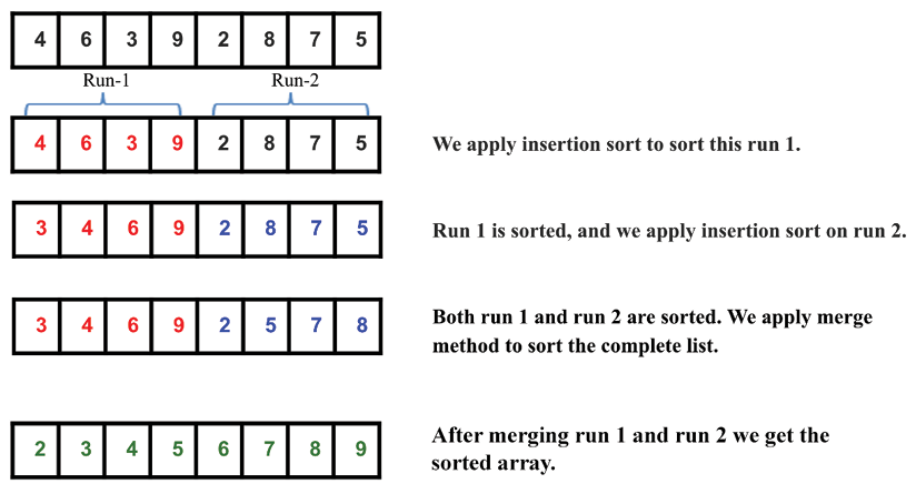
Figure 11.24: Illustration of an example array for the Timsort algorithm

Next, let’s discuss the implementation of the Timsort algorithm. Firstly, we implement the insertion sort algorithm and the merge method of the merge sort algorithm. The insertion sort algorithm has already been discussed in detail in previous sections. For completeness, it is given below again:

def Insertion_Sort(unsorted_list): 
    for index in range(1, len(unsorted_list)): 
        search_index = index 
        insert_value = unsorted_list[index] 
        while search_index > 0 and unsorted_list[search_index-1] > insert_value : 
            unsorted_list[search_index] = unsorted_list[search_index-1] 
            search_index -= 1 
        unsorted_list[search_index] = insert_value 
    return unsorted_list

In the above, the insertion sort method is responsible in sorting the run. Next, we present the merge method of the merge sort algorithm; this has been discussed in detail in Chapter 3, Algorithm Design Techniques and Strategies. This Merge() function is used to merge the sorted runs, and it is defined as follows:

def Merge(first_sublist, second_sublist):
    i = j = 0
    merged_list = []
    while i < len(first_sublist) and j < len(second_sublist):
        if first_sublist[i] < second_sublist[j]:
            merged_list.append(first_sublist[i])  
            i += 1  
        else:
            merged_list.append(second_sublist[j])  
            j += 1
    while i < len(first_sublist):  
        merged_list.append(first_sublist[i])  
        i += 1  
    while j < len(second_sublist):
        merged_list.append(second_sublist[j])  
        j += 1
    return merged_list

Next, let’s discuss the Timsort algorithm. Its implementation is given below. Let’s understand it bit by bit:

def Tim_Sort(arr, run):
    for x in range(0, len(arr), run):
        arr[x : x + run] = Insertion_Sort(arr[x : x + run]) 
    runSize = run    
    while runSize < len(arr):
        for x in range(0, len(arr), 2 * runSize):
            arr[x : x + 2 * runSize] = Merge(arr[x : x + runSize], arr[x + runSize: x + 2 * runSize]) 
            
        runSize = runSize * 2

In the above implementation, we firstly pass two parameters, the array that is to be sorted and the size of the run. Next, we use insertion sort to sort the individual subarrays by run size in the below code snippet:

for x in range(0, len(arr), run):
       arr[x : x + run] = Insertion_Sort(arr[x : x + run])

In the above code for the example list [4, 6, 3, 9, 2, 8, 7, 5], let’s say run size is 2, so we will have a total of four blocks/chunks/runs, and after exiting this loop, the array will be like this: [4, 6, 3, 9, 2, 8, 5, 7], indicating that all runs of size 2 are sorted. After that we initialize runSize and we iterate until runSize becomes equal to the array length. So, we use the merge method for combining the sorted small lists:

    runSize = run    
    while runSize < len(arr):
        for x in range(0, len(arr), 2 * runSize):
            arr[x : x + 2 * runSize] = Merge(arr[x : x + runSize], arr[x + runSize: x + 2 * runSize]) 
            
        runSize = runSize * 2

In the above code, the for loop is using the Merge function for merging the runs of size runSize. For the example above, the runSize is 2. In the first iteration, it will merge the left run from index (0 to 1) and right run from index (2 to 3) to form a sorted array from index (0 to 3), and the array will become [3, 4, 6, 9, 2, 8, 5, 7].

Further, in the second iteration, it will merge the left run from index (4 to 5) and the right run from index (6 to 7) to form a sorted run from index (4 to 7). After the second iteration the for loop will terminate and the array will become [3, 4, 6, 9, 2, 5, 7, 8], which indicates the array has been sorted from index (0 to 3) and (4 to 7).

Now we update the size of the run as 2*runSize and we repeat the same process for the updated runSize. So now, runSize is 4. Now, in the first iteration, it will merge the left run (index 0 to 3) and right run (index 4 to 7) to form a sorted array from index (0 to 7) and after this the for loop will terminate and the array will become [2, 3, 4, 5, 6, 7, 8, 9], which indicates the array has been sorted.

Now, runSize will become equal to the array length so the while loop will terminate, and at last, we will be left with the sorted array.

We can use the below code snippet to create a list, and then sort the list using the Timsort algorithm:

arr = [4, 6, 3, 9, 2, 8, 7, 5]
run = 2
Tim_Sort(arr, run) 
print(arr)

The output of the above code is as follows:

[2,3,4,5,6,7,8,9]

Timsort is very efficient for real-world applications since it has a worst-case complexity of O(n logn). Timsort is the best choice for sorting, even if the length of the given list is short. In that case, it uses the insertion sort algorithm, which is very fast for smaller lists, and the Timsort algorithm works fast for long lists due to the merge method; hence, the Timsort algorithm is a good choice for sorting due to its adaptability for sorting arrays of any length in real-world usage.

A comparison of the complexities of different sorting algorithms is given in the following table:

Table 11.1: Comparing the complexity of different sorting algorithms

Summary

In this chapter, we have explored important and popular sorting algorithms that are very useful for many real-world applications. We have discussed the bubble sort, insertion sort, selection sort, quicksort, and Timsort algorithms, along with explaining their implementation in Python. In general, the quicksort algorithm performs better than the other sorting algorithms, and the Timsort algorithm is the best choice to use in real-world applications.

In the next chapter, we will discuss selection algorithms.

Exercise

1. If an array arr = {55, 42, 4, 31} is given and bubble sort is used to sort the array elements, then how many iterations will be required to sort the array?
   1. 3
   2. 2
   3. 1
   4. 0
2. What is the worst-case complexity of bubble sort?
   1. O(n log n)
   2. O(log n)
   3. O(n)
   4. O(n²)
3. Apply quicksort to the sequence (56, 89, 23, 99, 45, 12, 66, 78, 34). What is the sequence after the first phase, and what pivot is the first element?
   1. 45, 23, 12, 34, 56, 99, 66, 78, 89
   2. 34, 12, 23, 45, 56, 99, 66, 78, 89
   3. 12, 45, 23, 34, 56, 89, 78, 66, 99
   4. 34, 12, 23, 45, 99, 66, 89, 78, 56
4. Quicksort is a ___________
   1. Greedy algorithm
   2. Divide and conquer algorithm
   3. Dynamic programming algorithm
   4. Backtracking algorithm
5. Consider a situation where a swap operation is very costly. Which of the following sorting algorithms should be used so that the number of swap operations is minimized?
   1. Heap sort
   2. Selection sort
   3. Insertion sort
   4. Merge sort
6. If the input array A = {15, 9, 33, 35, 100, 95, 13, 11, 2, 13} is given, using selection sort, what would the order of the array be after the fifth swap? (Note: it counts regardless of whether they exchange places or remain in the same position.)
   1. 2, 9, 11, 13, 13, 95, 35, 33, 15, 100
   2. 2, 9, 11, 13, 13, 15, 35, 33, 95, 100
   3. 35, 100, 95, 2, 9, 11, 13, 33, 15, 13
   4. 11, 13, 9, 2, 100, 95, 35, 33, 13, 13
7. What will be the number of iterations to sort the elements {44, 21, 61, 6, 13, 1} using insertion sort?
   1. 6
   2. 5
   3. 7
   4. 1
8. How will the array elements A= [35, 7, 64, 52, 32, 22] look after the second iteration, if the elements are sorted using insertion sort?
   1. 7, 22, 32, 35, 52, 64
   2. 7, 32, 35, 52, 64, 22
   3. 7, 35, 52, 64, 32, 22
   4. 7, 35, 64, 52, 32, 22

Join our community on Discord

Join our community’s Discord space for discussions with the author and other readers: https://packt.link/MEvK4