
2
Introduction to Algorithm Design
The objective of this chapter is to understand the principles of designing algorithms, and the importance of analyzing algorithms in solving real-world problems. Given input data, an algorithm is a step-by-step set of instructions that should be executed in sequence to solve a given problem.
In this chapter, we will also learn how to compare different algorithms and determine the best algorithm for the given use-case. There can be many possible correct solutions for a given problem, for example, we can have several algorithms for the problem of sorting n numeric values. So, there is no one algorithm to solve any real-world problem.
In this chapter, we will look at the following topics:
- Introducing algorithms
- Performance analysis of an algorithm
- Asymptotic notation
- Amortized analysis
- Choosing complexity classes
- Computing the running time complexity of an algorithm
Introducing algorithms
An algorithm is a sequence of steps that should be followed in order to complete a given task/problem.
It is a well-defined procedure that takes input data, processes it, and produces the desired output. A representation of this is shown in Figure 2.1.

Figure 2.1: Introduction to algorithms
Summarized below are some important reasons for studying algorithms:
- Essential for computer science and engineering
- Important in many other domains (such as computational biology, economics, ecology, communications, ecology, physics, and so on)
- They play a role in technology innovation
- They improve problem-solving and analytical thinking
There are two aspects that are of prime importance in solving a given problem. Firstly, we need an efficient mechanism to store, manage, and retrieve data, which is required to solve a problem (this comes under data structures); secondly, we require an efficient algorithm that is a finite set of instructions to solve that problem. Thus, the study of data structures and algorithms is key to solving any problem using computer programs. An efficient algorithm should have the following characteristics:
- It should be as specific as possible
- It should have each instruction properly defined
- There should not be any ambiguous instructions
- All the instructions of the algorithm should be executable in a finite amount of time and in a finite number of steps
- It should have clear input and output to solve the problem
- Each instruction of the algorithm should be integral in solving the given problem
Consider an example of an algorithm (an analogy) to complete a task in our daily lives; let us take the example of preparing a cup of tea. The algorithm to prepare a cup of tea can include the following steps:
- Pour water into the pan
- Put the pan on the stove and light the stove
- Add crushed ginger to the warming water
- Add tea leaves to the pan
- Add milk
- When it starts boiling, add sugar to it
- After 2-3 minutes, the tea can be served
The above procedure is one of the possible ways to prepare tea. In the same way, the solution to a real-world problem can be converted into an algorithm, which can be developed into computer software using a programming language. Since it is possible to have several solutions for a given problem, it should be as efficient as possible when it is to be implemented using software. Given a problem, there may be more than one correct algorithm, defined as the one that produces exactly the desired output for all valid input values. The costs of executing different algorithms may be different; it may be measured in terms of the time required to run the algorithm on a computer system and the memory space required for it.
There are primarily two things that one should keep in mind while designing an efficient algorithm:
- The algorithm should be correct and should produce the results as expected for all valid input values
- The algorithm should be optimal in the sense that it should be executed on the computer within the desired time limit, in line with an optimal memory space requirement
Performance analysis of the algorithm is very important for deciding the best solution for a given problem. If the performance of an algorithm is within the desired time and space requirements, it is optimal. One of the most popular and common methods of estimating the performance of an algorithm is through analyzing its complexity. Analysis of the algorithm helps us to determine which one is most efficient in terms of the time and space consumed.
Performance analysis of an algorithm
The performance of an algorithm is generally measured by the size of its input data, n, and the time and the memory space used by the algorithm. The time required is measured by the key operations to be performed by the algorithm (such as comparison operations), where key operations are instructions that take a significant amount of time during execution. Whereas the space requirement of an algorithm is measured by the memory needed to store the variables, constants, and instructions during the execution of the program.
Time complexity
The time complexity of the algorithm is the amount of time that an algorithm will take to execute on a computer system to produce the output. The aim of analyzing the time complexity of the algorithm is to determine, for a given problem and more than one algorithm, which one of the algorithms is the most efficient with respect to the time required to execute. The running time required by an algorithm depends on the input size; as the input size, n, increases, the runtime also increases. Input size is measured as the number of items in the input, for example, the input size for a sorting algorithm will be the number of items in the input. So, a sorting algorithm will have an increased runtime to sort a list of input size 5,000 than that of a list of input size 50.
The runtime of an algorithm for a specific input depends on the key operations to be executed in the algorithm. For example, the key operation for a sorting algorithm is a comparison operation that will take up most of the runtime, compared to assignment or any other operation. Ideally, these key operations should not depend upon the hardware, the operating system, or the programming language being used to implement the algorithm.
A constant amount of time is required to execute each line of code; however, each line may take a different amount of time to execute. In order to understand the running time required for an algorithm, consider the below code as an example:
|
Code |
Time required (Cost) |
|
|
Here, in statement 1 of the above example, if the condition is true then "data" will be printed, and if the condition is not true then the for loop will execute n times. The time required by the algorithm depends on the time required for each statement, and how many times a statement is executed. The running time of the algorithm is the sum of time required by all the statements. For the above code, assume statement 1 takes c1 amount of time, statement 2 takes c2 amount of time, and so on. So, if the ith statement takes a constant amount of time ci and if the ith statement is executed n times, then it will take cin time. The total running time T(n) of the algorithm for a given value of n (assuming the value of n is not zero or three) will be as follows.
T(n) = c1 + c3 + c4 x n + c5 x n
If the value of n is equal to zero or three, then the time required by the algorithm will be as follows.
T(n) = c1 + c2
Therefore, the running time required for an algorithm also depends upon what input is given in addition to the size of the input given. For the given example, the best case will be when the input is either zero or three, and in that case, the running time of the algorithm will be constant. In the worst case, the value of n is not equal to zero or three, then, the running time of the algorithm can be represented as a x n + b. Here, the values of a and b are constants that depend on the statement costs, and the constant times are not considered in the final time complexity. In the worst case, the runtime required by the algorithm is a linear function of n.
Let us consider another example, linear search:
def linear_search(input_list, element):
    for index, value in enumerate(input_list):
        if value == element:
            return index

    return -1
input_list = [3, 4, 1, 6, 14]
element = 4
print("Index position for the element x is:", linear_search(input_list,element))
The output in this instance will be as follows:
Index position for the element x is: 1
The worst-case running time of the algorithm is the upper-bound complexity; it is the maximum runtime required for an algorithm to execute for any given input. The worst-case time complexity is very useful in that it guarantees that for any input data, the runtime required will not take more time as compared to the worst-case running time. For example, in the linear search problem, the worst case occurs when the element to be searched is found in the last comparison or not found in the list. In this case, the running time required will linearly depend upon the length of the list, whereas, in the best case, the search element will be found in the first comparison.
The average-case running time is the average running time required for an algorithm to execute. In this analysis, we compute the average over the running time for all possible input values. Generally, probabilistic analysis is used to analyze the average-case running time of an algorithm, which is computed by averaging the cost over the distribution of all the possible inputs. For example, in the linear search, the number of comparisons at all positions would be 1 if the element to be searched was found at the 0th index; and similarly, the number of comparisons would be 2, 3, and so forth, up to n, respectively, for elements found at the 1, 2, 3, … (n-1) index positions. Thus, the average-case running time will be as follows.

For average-case, the running time required is also linearly dependent upon the value of n. However, in most real-world applications, worst-case analysis is mostly used, since it gives a guarantee that the running time will not take any longer than the worst-case running time of the algorithm for any input value.
Best-case running time is the minimum time needed for an algorithm to run; it is the lower bound on the running time required for an algorithm; in the example above, the input data is organized in such a way that it takes its minimum running time to execute the given algorithm.
Space complexity
The space complexity of the algorithm estimates the memory requirement to execute it on a computer to produce the output as a function of input data. The memory space requirement of an algorithm is one of the criteria used to decide how efficient it is. While executing the algorithm on the computer system, storage of the input is required, along with intermediate and temporary data in data structures, which are stored in the memory of the computer. In order to write a programming solution for any problem, some memory is required for storing variables, program instructions, and executing the program on the computer. The space complexity of an algorithm is the amount of memory required for executing and producing the result.
For computing the space complexity, consider the following example, in which, given a list of integer values, the function returns the square value of the corresponding integer number.
def squares(n):
    square_numbers = []
    for number in n:
        square_numbers.append(number * number)
    return square_numbers

nums = [2, 3, 5, 8 ]
print(squares(nums))
The output of the code is:
[4, 9, 25, 64]
In the above code, the algorithm will require allocating memory for the number of items in the input list. Say the number of elements in the input is n, then the space requirement increases with the input size, therefore, the space complexity of the algorithm becomes O(n).
Given two algorithms to solve a given problem, with all other requirements being equal, then the algorithm that requires less memory can be considered more efficient. For example, suppose there are two search algorithms, one has O(n) and another algorithm has O(nlogn) space complexity. The first algorithm is the better algorithm as compared to the second with respect to the space requirements. Space complexity analysis is important to understand the efficiency of an algorithm, especially for applications where the memory space requirement is high.
When the input size becomes large enough, the order of growth also becomes important. In such situations, we study the asymptotic efficiency of algorithms. Generally, algorithms that are asymptotically efficient are considered to be better algorithms for large-size inputs. In the next section, we will study asymptotic notation.
Asymptotic notation
To analyze the time complexity of an algorithm, the rate of growth (order of growth) is very important when the input size is large. When the input size becomes large, we only consider the higher-order terms and ignore the insignificant terms. In asymptotic analysis, we analyze the efficiency of algorithms for large input sizes considering the higher order of growth and ignoring the multiplicative constants and lower-order terms.
We compare two algorithms with respect to input size rather than the actual runtime and measure how the time taken increases with an increased input size. The algorithm which is more efficient asymptotically is generally considered a better algorithm as compared to the other algorithm. The following asymptotic notations are commonly used to calculate the running time complexity of an algorithm:
- θ notation: It denotes the worst-case running time complexity with a tight bound.
- Ο notation: It denotes the worst-case running time complexity with an upper bound, which ensures that the function never grows faster than the upper bound.
- Ω notation: It denotes the lower bound of an algorithm’s running time. It measures the best amount of time to execute the algorithm.
Theta notation
The following function characterizes the worst-case running time for the first example discussed in the Time complexity section:
T(n) = c1 + c3 x n + c5 x n
Here, for a large input size, the worst-case running time will be ϴ(n) (pronounced as theta of n). We usually consider one algorithm to be more efficient than another if its worst-case running time has a lower order of growth. Due to constant factors and lower-order terms, an algorithm whose running time has a higher order of growth might take less time for small inputs than an algorithm whose running time has a lower order of growth. For example, once the input size n becomes large enough, the merge sort algorithm performs better as compared to insertion sort with worst-case running times of ϴ(logn) and ϴ(n2 respectively.)
Theta notation (ϴ) denotes the worst-case running time for an algorithm with a tight bound. For a given function F(n), the asymptotic worst-case running time complexity can be defined as follows.
![]()
iff there exists constants n0, c1, and c2 such that:
![]()
The function T(n) belongs to a set of functions ϴ(F(n)) if there exists positive constants c1 and c2 such that the value of T(n) always lies in between c1F(n) and c2F(n) for all large values of n. If this condition is true, then we say F(n) is asymptotically tight bound for T(n).
Figure 2.2 shows the graphic example of the theta notation (ϴ). It can be observed from the figure that the value of T(n) always lies in between c1F(n) and c2F(n) for values of n greater than n0.

Figure 2.2: Graphical example of theta notation (ϴ)
Let us consider an example to understand what should be the worst case running time complexity with the formal definition of theta notation for a given function:
![]()
In order to determine the time complexity with the ϴ notation definition, we have to first identify the constants c1, c2, n0 such that
![]()
Dividing by n2 will produce:
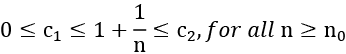
By choosing c1 = 1, c2 = 2, and n0 = 1, the following condition can satisfy the definition of theta notation.
![]()
That gives:
![]()
Consider another example to find out the asymptotically tight bound (ϴ) for another function:

In order to identify the constants c1, c2, and n0, such that they satisfy the condition:

By choosing c1 = 1/5, c2 =1, and n0 = 1, the following condition can satisfy the definition of theta notation:
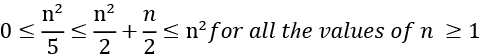

So, the following is true:

It shows that the given function has the complexity of ϴ(n2) as per the definition of theta notation.
So, the theta notation provides a tight bound for the time complexity of an algorithm. In the next section, we will discuss Big O notation.
Big O notation
We have seen that the theta notation is asymptotically bound from the upper and lower sides of the function whereas the Big O notation characterizes the worst-case running time complexity, which is only the asymptotic upper bound of the function. Big O notation is defined as follows. Given a function F(n), the T(n) is a Big O of function F(n), and we define this as follows:
T(n) = O(F(n))
iff there exists constants n0 and c such that:
![]()
In Big O notation, a constant multiple of F(n) is an asymptotic upper bound on T(n), and the positive constants n0 and c should be in such a way that all values of n greater than n0 always lie on or below function c*F(n).
Moreover, we only care what happens at higher values of n. The variable n0 represents the threshold below which the rate of growth is not important. The plot shown in Figure 2.3 shows a graphical representation of function T(n) with a varying value of n. We can see that T(n) = n2 + 500 = O(n2), with c = 2 and n0 being approximately 23.

Figure 2.3: Graphical example of O notation
In O notation, O(F(n)) is really a set of functions that includes all functions with the same or smaller rates of growth than F(n). For example, O(n2) also includes O(n), O(log n), and so on. However, Big O notation should characterize a function as closely as possible, for example, it is true that function F(n) = 2n3+2n2+5 is O(n4), however, it is more accurate that F(n) is O(n3).
In the following table, we list the most common growth rates in order from lowest to highest.
|
Time Complexity |
Name |
|
|
Constant |
|
|
Logarithmic |
|
|
Linear |
|
|
Linear-logarithmic |
|
|
Quadratic |
|
|
Cubic |
|
|
Exponential |
Table 2.1: Runtime complexity of different functions
Using Big O notation, the running time of an algorithm can be computed by analyzing the structure of the algorithm. For example, a double nested loop in an algorithm will have an upper bound on the worst-case running time of O(n2), since the values of i and j will be at most n, and both the loops will run n2 times as shown in the below example code:
for i in range(n):
    for j in range(n):
        print("data")
Let us consider a few examples in order to compute the upper bound of a function using the O-notation:
- Find the upper bound for the function:
T(n) = 2n + 7
Solution: Using O notation, the condition for the upper bound is:
T(n) <= c * F(n)
This condition holds true for all values of n > 7 and c=3.
2n + 7 <= 3n This is true for all values of n, with c=3, n0=7
T(n) = 2n+7 = O(n)
- Find F(n) for functions T(n) =2n+5 such that T(n) = O(F(n)).
Solution: Using O notation, the condition for the upper bound is T(n) <=c * F(n).
Since, 2n+5 ≤ 3n, for all n ≥ 5.
The condition is true for c=3, n0=5.
2n + 5 ≤ O(n)
F(n) = n
- Find F(n) for the function T(n) = n2 +n, such that T(n) = O(F(n)).
Solution: Using O notation, since, n2+ n ≤ 2n2, for all n ≥ 1 (with c = 2, n0=2)
n2+ n ≤ O(n2)
F(n) = n2
- Prove that f(n) =2n3 - 6n ≠ O(n2).
Solution: Clearly, 2n3-6n ≥ n2, for n ≥ 2. So it cannot be true that 2n3 - 6n ≠ O(n2).
- Prove that: 20n2+2n+5 = O(n2).
Solution: It is clear that:
20n2 + 2n + 5 <= 21n2 for all n > 4 (let c = 21 and n0 = 4)
n2 > 2n + 5 for all n > 4
So, the complexity is O(n2).
So, Big-O notation provides an upper bound on a function, which ensures that the function never grows faster than the upper-bounded function. In the next section, we will discuss Omega notation.
Omega notation
Omega notation (Ω) describes an asymptotic lower bound on algorithms, similar to the way in which Big O notation describes an upper bound. Omega notation computes the best-case runtime complexity of the algorithm. The Ω notation (Ω(F(n)) is pronounced as omega of F of n), is a set of functions in such a way that there are positive constants n0 and c such that for all values of n greater than n0, T(n) always lies on or above a function to c*F(n).
T(n) = Ω (F(n))
Iff constants n0 and c are present, then:
![]()
Figure 2.4 shows the graphical representation of the omega (Ω) notation. It can be observed from the figure that the value of T(n) always lies above cF(n) for values of n greater than n0.

Figure 2.4: The graphical representation of Ω notation
If the running time of an algorithm is Ω(F(n)), it means that the running time of the algorithm is at least a constant multiplier of F(n) for sufficiently large values of input size (n). The Ω notation gives a lower bound on the best-case running time complexity of a given algorithm. It means that the running time for a given algorithm will be at least F(n) without depending upon the input.
In order to understand the Ω notation and how to compute the lower bound on the best-case runtime complexity of an algorithm:
- Find F(n) for the function T(n) =2n2 +3 such that T(n) = Ω(F(n)).
Solution: Using the Ω notation, the condition for the lower bound is:
c*F(n) ≤ T(n)
This condition holds true for all values of n greater than 0, and c=1.
0 ≤ cn2 ≤ 2n2 +3, for all n ≥ 0
2n2 +3 = Ω(n2)
F(n)=n2
- Find the lower bound for T(n) = 3n2.
Solution: Using the Ω notation, the condition for the lower bound is:
c*F(n) ≤ T(n)
Consider 0 ≤ cn2 ≤ 3n2. The condition for Ω notation holds true for all values of n greater than 1, and c=2.
cn2 ≤ 3n2 (for c = 2 and n0 = 1)
3n2 = Ω(n2)
- Prove that 3n = Ω(n).
Solution: Using the Ω notation, the condition for the lower bound is:
c*F(n) ≤ T(n)
Consider 0 ≤ c*n ≤ 3n. The condition for Ω notation holds true for all values of n greater than 1, and c=1.
cn2 ≤ 3n2 ( for c = 2 and n0 = 1)
3n = Ω(n)
The Ω notation is used to describe that at least a certain amount of running time will be taken by an algorithm for a large input size. In the next section, we will discuss amortized analysis.
Amortized analysis
In the amortized analysis of an algorithm, we average the time required to execute a sequence of operations with all the operations of the algorithm. This is called amortized analysis. Amortized analysis is important when we are not interested in the time complexity of individual operations but we are interested in the average runtime of sequences of operations. In an algorithm, each operation requires a different amount of time to execute. Certain operations require significant amounts of time and resources while some operations are not costly at all. In amortized analysis, we analyze algorithms considering both the costly and less costly operations in order to analyze all the sequences of operations. So, an amortized analysis is the average performance of each operation in the worst case considering the cost of the complete sequence of all the operations. Amortized analysis is different from average-case analysis since the distribution of the input values is not considered. An amortized analysis gives the average performance of each operation in the worst case.
There are three commonly used methods for amortized analysis:
- Aggregate analysis. In aggregate analysis, the amortized cost is the average cost of all the sequences of operations. For a given sequence of n operations, the amortized cost of each operation can be computed by dividing the upper bound on the total cost of n operations with n.
- The accounting method. In the accounting method, we assign an amortized cost to each operation, which may be different than their actual cost. In this, we impose an extra charge on early operations in the sequence and save “credit cost,” which is used to pay expensive operations later in the sequence.
- The potential method. The potential method is like the accounting method. We determine the amortized cost of each operation and impose an extra charge to early operations that may be used later in the sequence. Unlike the accounting method, the potential method accumulates the overcharged credit as “potential energy” of the data structure as a whole instead of storing credit for individual operations.
In this section, we had an overview of amortized analysis. Now we will discuss how to compute the complexity of different functions with examples in the next section.
Composing complexity classes
Normally, we need to find the total running time of complex operations and algorithms. It turns out that we can combine the complexity classes of simple operations to find the complexity class of more complex, combined operations. The goal is to analyze the combined statements in a function or method to understand the total time complexity of executing several operations. The simplest way to combine two complexity classes is to add them. This occurs when we have two sequential operations. For example, consider the two operations of inserting an element into a list and then sorting that list. Assuming that inserting an item occurs in O(n) time, and sorting in O(nlogn) time, then we can write the total time complexity as O(n + nlogn); that is, we bring the two functions inside the O(…), as per Big O computation. Considering only the highest-order term, the final worst-case complexity becomes O(nlogn).
If we repeat an operation, for example in a while loop, then we multiply the complexity class by the number of times the operation is carried out. If an operation with time complexity O(f(n)) is repeated O(n) times, then we multiply the two complexities: O(f(n) * O(n)) = O(nf(n)). For example, suppose the function f(n) has a time complexity of O(n2) and it is executed n times in a for loop, as follows:
for i in range(n):
        f(...)
The time complexity of the above code then becomes:
O(n2) x O(n) = O(n x n2) = O(n3)
Here, we are multiplying the time complexity of the inner function by the number of times this function executes. The runtime of a loop is at most the runtime of the statements inside the loop multiplied by the number of iterations. A single nested loop, that is, one loop nested inside another loop, will run n2 times, such as in the following example:
for i in range(n):
    for j in range(n)
        #statements
If each execution of the statements takes constant time, c, i.e. O(1), executed n x n times, we can express the running time as follows:
c x n x n = c x n2 = O(n2)
For consecutive statements within nested loops, we add the time complexities of each statement and multiply by the number of times the statement is executed—as in the following code, for example:
def fun(n):
   for i in range(n):  #executes n times
      print(i)     #c1
   for i in range(n):
      for j in range(n):
         print(j)  #c2
This can be written as: c1n + c2 *n2 = O(n2).
We can define (base 2) logarithmic complexity, reducing the size of the problem by half, in constant time. For example, consider the following snippet of code:
i = 1
while i <= n:
    i = i*2
    print(i)
Notice that i is doubling in each iteration. If we run this code with n = 10, we see that it prints out four numbers: 2, 4, 8, and 16. If we double n, we see it prints out five numbers. With each subsequent doubling of n, the number of iterations is only increased by 1. If we assume that the loop has k iterations, then the value of n will be 2n. We can write this as follows:
![]()
![]()
![]()
From this, the worst-case runtime complexity of the above code is equal to O(log(n)).
In this section, we have seen examples to compute the running time complexity of different functions. In the next section, we will take examples to understand how to compute the running time complexity of an algorithm.
Computing the running time complexity of an algorithm
To analyze an algorithm with respect to the best-, worst-, and average-case runtime of the algorithm, it is not always possible to compute these for every given function or algorithm. However, it is always important to know the upper-bound worst-case runtime complexity of an algorithm in practical situations; therefore, we focus on computing the upper-bound Big O notation to compute the worst-case runtime complexity of an algorithm:
- Find the worst-case runtime complexity of the following Python snippet:
# loop will run n times for i in range(n): print("data") #constant timeSolution: The runtime for a loop, in general, takes the time taken by all statements in the loop, multiplied by the number of iterations. Here, total runtime is defined as follows:
T(n) = constant time (c) * n = c*n = O(n)
- Find the time complexity of the following Python snippet:
for i in range(n): for j in range(n): # This loop will also run for n times print("run")Solution: O(n2). The
printstatement will be executed n2 times, n times for the inner loop, and, for each iteration of the outer loop, the inner loop will be executed.
- Find the time complexity of the following Python snippet:
for i in range(n): for j in range(n): print("run fun") breakSolution: The worst-case complexity will be O(n) since the
printstatement will run n times because the inner loop executes only once due to abreakstatement.
- Find the time complexity of the following Python snippet:
def fun(n): for i in range(n): print("data") #constant time #outer loop execute for n times for i in range(n): for j in range(n): #inner loop execute n times print("run fun") #constant timeSolution: Here, the
printstatements will execute n times in the first loop and n2 times for the second nested loop. Here, the total time required is defined as the following:T(n) = constant time (c1) * n + c2*n*n
c1 n + c2 n2 = O(n2)
- Find the time complexity of the following Python snippet:
if n == 0: #constant time print("data") else: for i in range(n): #loop run for n times print("structure")Solution: O(n). Here, the worst-case runtime complexity will be the time required for the execution of all the statements; that is, the time required for the execution of the
if-elseconditions, and theforloop. The time required is defined as the following:T(n) = c1 + c2 n = O(n)
- Find the time complexity of the following Python snippet:
i = 1 j = 0 while i*i < n: j = j +1 i = i+1 print("data")Solution: O(
 ). The loop will terminate based on the value of
 i; the loop will iterate based on the condition:
T(n) = O(
 )
)
- Find the time complexity of the following Python snippet:
i = 0 for i in range(int(n/2), n): j = 1 while j+n/2 <= n: k = 1 while k < n: k *= 2 print("data") j += 1Solution: Here, the outer loop will execute n/2 times, the middle loop will also run n/2 times, and the innermost loop will run for log(n) time. So, the total running time complexity will be O(n*n*logn):
O(n2logn)
Summary
In this chapter, we have looked at an overview of algorithm design. The study of algorithms is important because it trains us to think very specifically about certain problems. It is conducive to increasing our problem-solving abilities by isolating the components of a problem and defining the relationships between them. In this chapter, we discussed different methods for analyzing algorithms and comparing algorithms. We also discussed asymptotic notations, namely: Big Ο, Ω, and θ notation.
In the next chapter, we will discuss algorithm design techniques and strategies.
Exercises
- Find the time complexity of the following Python snippets:
-
i=1 while(i<n): i*=2 print("data") -
i =n while(i>0): print('complexity') i/ = 2 -
for i in range(1,n): j = i while(j<n): j*=2 -
i=1
while(i<n):
    print('python')
        i = i**2
Join our community on Discord
Join our community’s Discord space for discussions with the author and other readers: https://packt.link/MEvK4
