We can use dimensionality reduction algorithms for a slightly different task – data compression with information loss. This can be easily demonstrated when applying the PCA algorithm to images. Let's implement PCA from scratch with the Dlib library using SVD decomposition. We can't use an existing implementation because it performs normalization in a way we can't fully control.

First, we need to load an image and transform it into matrix form:

 void PCACompression(const std::string& image_file, long target_dim) {
     array2d<Dlib::rgb_pixel> img;
     load_image(img, image_file);
 
     array2d<unsigned char> img_gray;
     assign_image(img_gray, img);
     save_png(img_gray, "original.png");
 
     array2d<DataType> tmp;
     assign_image(tmp, img_gray);
     Matrix img_mat = Dlib::mat(tmp);
     img_mat /= 255.;  // scale
 
     std::cout << "Original data size " << img_mat.size() << std::endl;

After we've loaded the RGB image, we convert it into grayscale and transform its values into floating points. The next step is to transform the image matrix into samples that we can use for PCA training. This can be done by splitting the image into rectangular patches that are 8 x 8 in size with the Dlib::subm() function and then flattening them with the Dlib::reshape_to_column_vector() function:

 std::vector<Matrix> data;
 int patch_size = 8;
 
 for (long r = 0; r < img_mat.nr(); r += patch_size) {
     for (long c = 0; c < img_mat.nc(); c += patch_size) {
         auto sm = Dlib::subm(img_mat, r, c, patch_size, patch_size);
         data.emplace_back(Dlib::reshape_to_column_vector(sm));
     }
 }

When we have our samples, we can normalize them by subtracting the mean and dividing them by their standard deviation. We can make these operations vectorized by converting our vector of samples into the matrix type. We do this with the Dlib::mat() function:

 // normalize data
 auto data_mat = mat(data);
 Matrix m = mean(data_mat);
 Matrix sd = reciprocal(sqrt(variance(data_mat)));
 
 matrix<decltype(data_mat)::type, 0, 1, decltype(data_mat)::mem_manager_type>
 x(data_mat);
 for (long r = 0; r < x.size(); ++r)
   x(r) = pointwise_multiply(x(r) - m, sd);

After we've prepared the data samples, we calculate the covariance matrix with the Dlib::covariance() function and perform SVD with the Dlib::svd() function. The SVD results are the eigenvalues matrix and the eigenvectors matrix. We sorted the eigenvectors according to the eigenvalues and left only a small number (in our case, 10 of them) of eigenvectors correspondent to the biggest eigenvalues. The number of eigenvectors we left is the number of dimensions in the new feature space:

 Matrix temp, eigen, pca;
 // Compute the svd of the covariance matrix
 Dlib::svd(covariance(x), temp, eigen, pca);
 Matrix eigenvalues = diag(eigen);
 
 rsort_columns(pca, eigenvalues);
 
 // leave only required number of principal components
 pca = trans(colm(pca, range(0, target_dim)));

Our PCA transformation matrix is called pca. We used it to reduce the dimensions of each of our samples with simple matrix multiplication. Look at the following cycle and notice the pca * data[i] operation:

 // dimensionality reduction
 std::vector<Matrix> new_data;
 size_t new_size = 0;
 new_data.reserve(data.size());
 for (size_t i = 0; i < data.size(); ++i) {
   new_data.emplace_back(pca * data[i]);
   new_size += static_cast<size_t>(new_data.back().size());
 }
 
 std::cout << "New data size " << new_size + 
     static_cast<size_t>(pca.size())
 << std::endl;

Our data has been compressed and we can see its new size in the console output. Now, we can restore the original dimension of the data to be able to see the image. To do this, we need to use the transposed PCA matrix to multiply the reduced samples. Also, we need to denormalize the restored sample to get actual pixel values. This can be done by multiplying the standard deviation and adding the mean we got from the previous steps:

 auto pca_matrix_t = Dlib::trans(pca);
 Matrix isd = Dlib::reciprocal(sd);
 for (size_t i = 0; i < new_data.size(); ++i) {
   Matrix sample = pca_matrix_t * new_data[i];
   new_data[i] = Dlib::pointwise_multiply(sample, isd) + m;
 }

After we've restored the pixel values, we reshape them and place them in their original location in the image:

     size_t i = 0;
     for (long r = 0; r < img_mat.nr(); r += patch_size) {
       for (long c = 0; c < img_mat.nc(); c += patch_size) {
         auto sm = Dlib::reshape(new_data[i], patch_size, patch_size);
         Dlib::set_subm(img_mat, r, c, patch_size, patch_size) = sm;
         ++i;
       }
     }
 
     img_mat *= 255.0;
     assign_image(img_gray, img_mat);
     equalize_histogram(img_gray);
     save_png(img_gray, "compressed.png");
 }

Let's look at the result of compressing a standard test image that is widely used in image processing. The following is the Lena 512 x 512 image:

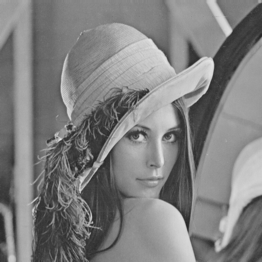
Its original grayscaled size is 262,144 bytes. After we perform PCA compression with only 10 principal components, its size becomes 45,760 bytes. We can see the result in the following image:

Here, we can see that most of the essential visual information was preserved, despite the high compression rate.