Logistic regression determines the degree of dependence between the categorical dependent and one or more independent variables by using the logistic function. It aims to find the values of the coefficients for the input variables, as with linear regression. The difference, in the case of logistic regression, is that the output value is converted by using a non-linear (logistic) function. The logistic function essentially looks like a big letter S and converts any value to a number in a range from 0 to 1. This property is useful because we can apply the rule to the output of the logistic function to bind 0 and 1 to a class prediction. The following screenshot shows a logistic function graph:

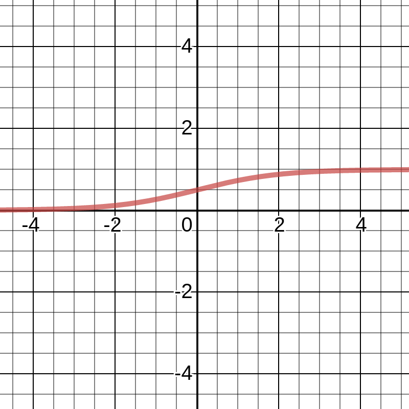
For example, if the result of the function is less than 0.5, then the output is 0. Prediction is not just a simple answer (+1 or -1) either, and we can interpret it as a probability of being classified as +1.

In many tasks, this interpretation is an essential business requirement. For example, in the task of credit scoring, where logistic regression is traditionally used, the probability of a loan being defaulted on is a common prediction. As with the case of linear regression, logistic regression performs the task better if outliers and correlating variables are removed. The logistic regression model can be quickly trained and is well suited for binary classification problems.

The basic idea of a linear classifier is that the feature space can be divided by a hyperplane into two half-spaces, in each of which one of the two values of the target class is predicted. If we can divide a feature space without errors, then the training set is called linearly separable. Logistic regression is a unique type of a linear classifier, but it is able to predict the probability of , attributing the example of to the class +, as illustrated here:

Consider the task of binary classification, with labels of the target class denoted by +1 (positive examples) and -1 (negative examples). We want to predict the probability of ; so, for now, we can build a linear forecast using the following optimization technique: . So, how do we convert the resulting value into a probability whose limits are [0, 1]? This approach requires a specific function. In the logistic regression model, the specific function is used for this.

Let's denote P(X) by the probability of the occurring event X. The probability odds ratio OR(X) is determined from . This is the ratio of the probabilities of whether the event will occur or not. We can see that the probability and the odds ratio both contain the same information. However, while P(X) is in the range of 0 to 1, OR(X) is in the range of 0 to . If you calculate the logarithm of OR(X) (known as the logarithm of the odds, or the logarithm of the probability ratio), it is easy to see that the following applies: .

Using the logistic function to predict the probability of , it can be obtained from the probability ratio (for the time being, let's assume we have the weights too) as follows:

So, the logistic regression predicts the probability of classifying a sample to the + class as a sigmoid transformation of a linear combination of the model weights vector, as well as the sample's features vector, as follows:

From the maximum likelihood principle, we can obtain an optimization problem that the logistic regression solves—namely, the minimization of the logistic loss function. For the - class, the probability is determined by a similar formula, as illustrated here:

The expressions for both classes can be combined into one, as illustrated here:

Here, the expression is called the margin of classification of the  object. The classification margin can be understood as a model's confidence in the object's classification. An interpretation of this margin is as follows:

• If the margin vector's absolute value is large and is positive, the class label is set correctly, and the object is far from the separating hyperplane. Such an object is therefore classified confidently.
• If the margin is large (by modulo) but is negative, then the class label is set incorrectly. The object is far from the separating hyperplane. Such an object is most likely an anomaly.
• If the margin is small (by modulo), then the object is close to the separating hyperplane. In this case, the margin sign determines whether the object is correctly classified.

In the discrete case, the likelihood function can be interpreted as the probability that the sample  X₁ , . . . , X_n is equal to x₁ , . . . , x_n in the given set of experiments. Furthermore, this probability depends on θ, as illustrated here:

The maximum likelihood estimate for the unknown parameter is called the value of , for which the function reaches its maximum (as a function of θ, with fixed ), as illustrated here:

Now, we can write out the likelihood of the sample—namely, the probability of observing the given vector in the sample . We make one assumption—objects arise independently from a single distribution, as illustrated here:

Let's take the logarithm of this expression since the sum is much easier to optimize than the product, as follows:

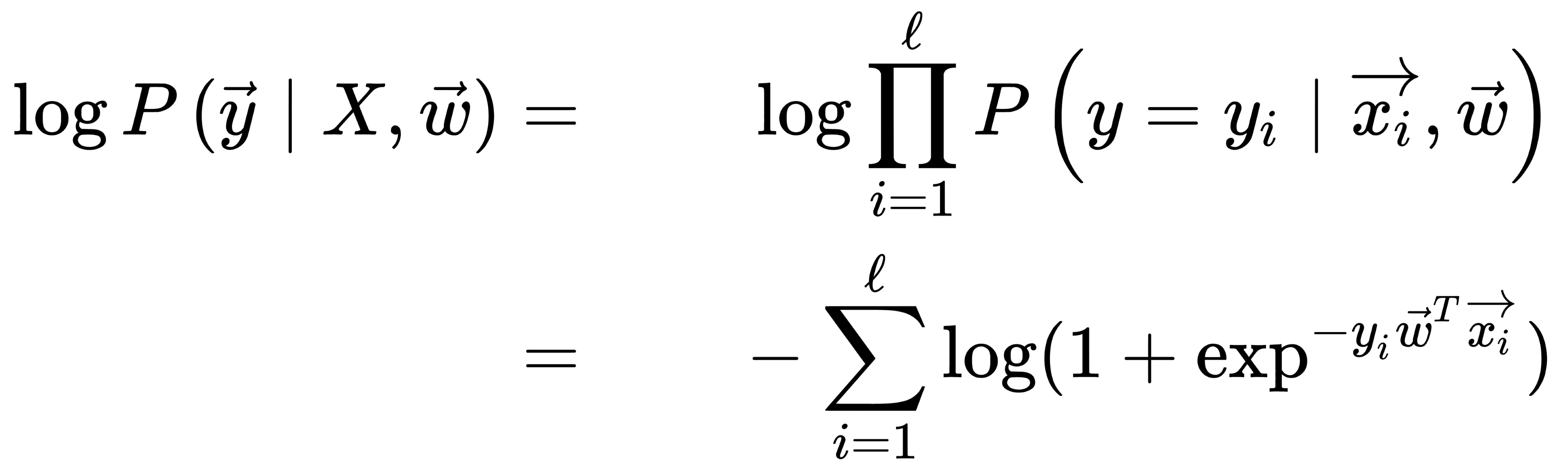
In this case, the principle of maximizing the likelihood leads to a minimization of the expression, as illustrated here:

This formula is a logistic loss function, summed over all objects of the training sample. Usually, it is a good idea to add some regularization to a model to deal with overfitting. L2 regularization of logistic regression is arranged in much the same way as linear regression (ridge regression). However, it is common to use the controlled variable decay parameter C that is used in SVM models, where it denotes soft margin parameter denotation. So, for logistic regression, C is equal to the inverse regularization coefficient . The relationship between C and  would be the following: lowering C would strengthen the regularization effect. Therefore, instead of the functional , the following function should be minimized:

For this function minimization, we can apply different methods—for example, the method of least squares, or the gradient descent (GD) method. The vital issue with logistic regression is that it is generally a linear classifier, in order to deal with non-linear decision boundaries, which typically use polynomial features with original features as a basis for them. This approach was discussed in the earlier chapters when we discussed polynomial regression.