The goal of an RNN is consistent data usage under the assumption that there is some dependency between consecutive data elements. In traditional neural networks, it is understood that all inputs and outputs are independent. But for many tasks, this independence is not suitable. If you want to predict the next word in a sentence, for example, knowing the sequence of words preceding it is the most reliable way to do so. RNNs are recurrent because they perform the same task for each element of the sequence, and the output is dependent on previous calculations. 

In other words, RNNs are networks that have feedback loops and memory. RNNs use memory to take into account prior information and calculations results. The idea of a recurrent network can be represented as follows:

In the preceding diagram, a fragment of the neural network,  (a layer of neurons with a sigmoidal activation function), takes the input value, , and returns the value, . The presence of feedback allows us to transfer information from one timestep of the network to another timestep. A recurrent network can be considered several copies of the same network, each of which transfers information to a subsequent copy. Here's what happens when we expand the feedback:

This can be represented in further detail as follows:

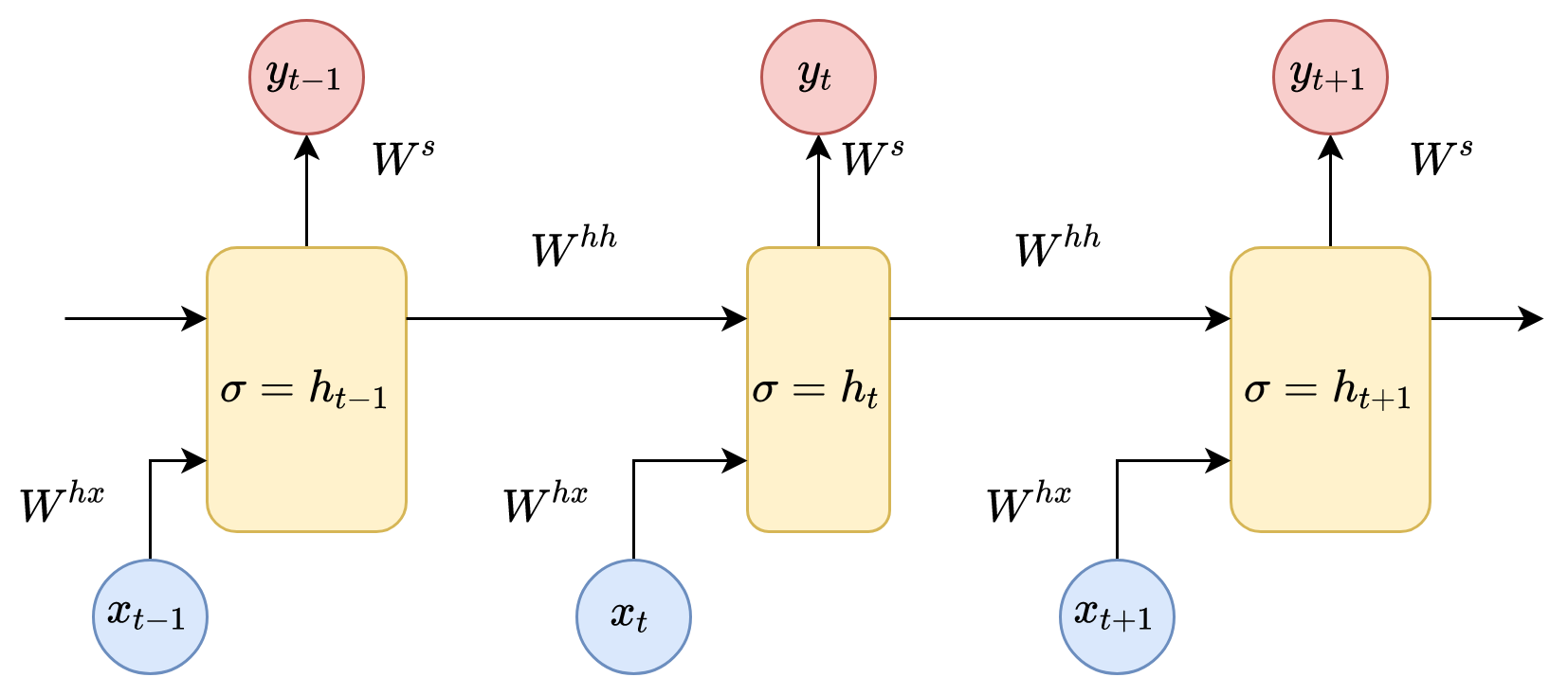
Here, we can see the input data vectors, . Each vector at each step has a hidden state vector, . We call this pairing a module. The hidden state in each RNN module is a function of the input vector and the hidden state vector from the previous step, as follows:

If we look at the superscript, we can see that there is a weight matrix, , which we multiply by the input value, and there is a recurrent weight matrix, , which is multiplied by a hidden state vector from the previous step. These recurrent weight matrices are the same at every step. This concept is a key component of an RNN. If you think about this carefully, this approach is significantly different from, say, traditional two-layer neural networks. In this case, we usually select a separate matrix, W, for each layer: W₁ and W₂. Here, the recurrent matrix of weights is the same for the entire network. denotes a neural network layer with a sigmoid as an activation function.

Furthermore, another weight matrix, , is used to obtain the output values, y, of each module, which are multiplied by h:

One of the attractive ideas of RNNs is that they potentially know how to connect previous information with the task at hand. For example, in the task of video flow analysis, knowledge of the previous frame of the video can help in understanding the current frame (knowing previous object positions can help us predict their new positions). The ability of RNNs to use prior information is not absolute and usually depends on some circumstances, which we will discuss in the following sections.

Sometimes, to complete the current task, we need only recent information. Consider, for example, a language model trying to predict the next word based on the previous words. If we want to predict the last word in the phrase, clouds are floating in the sky, we don't need a broader context; in this case, the last word is almost certainly sky. In this case, we could say that the distance between the relevant information and the subject of prediction is small, which means that RNNs can learn how to use information from the past.

But sometimes, we need more context. Suppose we want to predict the last word in the phrase, I speak French. Further back in the same text is the phrase, I grew up in France. The context, therefore, suggests that the last word should likely be the name of the country's language. However, this may have been much further back in the text – possibly on a different paragraph or page – and as that gap between the crucial context and the point of its application grows, RNNs lose their ability to bind information accurately.

In theory, RNNs should not have problems with long-term processing dependencies. A person can carefully select network parameters to solve artificial problems of this type. Unfortunately, in practice, training the RNN with these parameters seems impossible due to the vanishing gradient problem. This problem was investigated in detail by Sepp Hochreiter (1991) and Yoshua Bengio et al. (1994). They found that the lower the gradient that's used in the backpropagation algorithms, the more difficult it is for the network to update its weights and the longer the training time will be. There are different reasons why we can get low gradient values during the training process, but one of the main reasons is the network size. For RNNs, it is the most crucial parameter because it depends on the size of the input sequence we use. The longer the sequence that we use is, the bigger the network we get is. Fortunately, there are methods we can use to deal with this problem in RNNs, all of which we will discuss later in this chapter.