Text data offers a very unique proposition by not providing any direct representation available for it in terms of numbers. Computers only understand numbers. Representing text using numbers is a challenge. At the same time, it is an opportunity to invent and try out approaches to represent text so that the maximum information can be captured in the process. In this chapter, we will look at how text and math interface. Let's take baby steps toward transforming text data into mathematical data structures that will provide insights on how to actually represent text using numbers and, consequently, build Natural Language Processing (NLP) models.

Pause for a moment here and dwell on how would you try to solve it.

As we progress toward the end of this chapter, we will be better equipped to handle text data as we understand techniques including count vectorization and term frequency-inverse document frequency (TF-IDF) vectorization, among others.

Before we proceed and discuss various possible approaches such as count vectors and TF-IDF vectors in this chapter and more approaches such as Word2vec in future chapters, we need to understand two supremely important concepts that validate every language. These are syntax and semantics. Syntax defines the grammatical structures or the set of rules defining a language. It can be thought of as a set of guiding principles that define how words can be put in each other's vicinity to form sentences or phrases. However, syntactically correct sentences may not be meaningful. Semantics is the part that takes care of the meanings and defines how to put words together so that they actually make sense when organized based on the available syntactical rules.

In this chapter, we will primarily focus on the syntactical aspects, where we use information such as how many times a word occurred in a document or in a set of documents as potential features to represent documents. Let's see how these approaches pan out in solving the representation problem we have.

The following topics will be covered in this chapter:

• Understanding vectors and matrices
• Exploring the Bag-of-Words (BoW) architecture
• TF-IDF vectors
• Distance/similarity calculation between document vectors
• One-hot vectorization
• Building a basic chatbot

Technical requirements

The code files for this chapter can be found at the following GitHub link: https://github.com/PacktPublishing/Hands-On-Python-Natural-Language-Processing/tree/master/Chapter04.

Understanding vectors and matrices

The introduction to this chapter touched upon the challenge of representing text data in a mathematical form. Two of the most popular data structures used with text data are vectors and matrices. We will now have a look at each one of these in detail.

Vectors

Vectors are a one-dimensional array of numbers in which each number could be identified by its respective indices. They are typically represented as a column enclosed in square brackets, as shown here:

In this example, the x vector has three elements, and these three elements store information about the vector. Mathematicians abstract vectors as an object in space, where each element of the vector represents the projection of that vector along a given axis. We often use the term Rⁿ to define a vector, where R is a representation mechanism and n denotes the number of dimensions used to describe the vector. In general, Rⁿ is the set of all n-tuples of real numbers.

In the preceding example, the x vector is in R³, meaning the vector is in a three-dimensional space and its projection along the three axes is x1, x2, and x3. Once an object is abstracted as a vector, it must satisfy all vector properties, and we can perform any vector operation on it.

For example, let's assume we have height and weight data on two people—Person A and Person B, as shown in the following table:

We can assume a two-dimensional space where these two persons are represented by two vectors, as shown in the following screenshot. The respective height and weight of a person can be thought of as the coordinates that determine their position in the R² space:

If we also had the body temperature of these people, we could have abstracted this in R³space, which would have required a three-dimensional visualization. Vectorizationenables us to analyze subjects by using vector properties and operations such as magnitude, similarity, dissimilarity, and so on. Although visualizing vectors in a space greater than R³ is not humanly possible, all vector properties hold true for any dimensional space, and therefore we are not limited by the number of features of a given subject to transform data into vectors.

All this is great, but how is this going to help us with text analysis?

We have already discussed tokenization in Chapter 3, Building Your NLP Vocabulary. A tokenized text document could be abstracted as a vector in an n-dimensional space where each dimension (axis) in the space corresponds to a unique token of that document. The vector's projection along a given axis (coordinate) would be the count of that unique token in the text document. Once vectorized, the text document could be analyzed along with other text document vectors, using vector math.

Matrices

Matrices are an extension of arrays. They are a rectangular array of numbers wherein each number is identified by two indices. Like vectors, matrices are also represented using squared brackets, but matrices have both rows and columns, as shown in the following screenshot:

A matrix with height m and width n is said to be in R^{m x n} (the preceding matrix belongs to R^{3 x 2}). In the context of text analysis, matrices are used frequently to represent and analyze text data. Typically, each document vector is represented as a row of a matrix. In the following example, we have read three (small) documents in our system and have used the CountVectorizer module of the sklearn library to represent this data in a matrix format. The CountVectorizer module helps us vectorize each document and then combine each document vector to create the matrix.

The following code block will give you some perspective about building vectors and matrices based on text data. These will be discussed in detail in the later sections of this chapter:

from sklearn.feature_extraction.text import CountVectorizer
X = ("Computers can analyze text",
    "They do it using vectors and matrices",
    "Computers can process massive amounts of text data")
vectorizer = CountVectorizer(stop_words='english')
X_vec = vectorizer.fit_transform(X)
print(vectorizer.vocabulary_)
print(X_vec.todense()) 

The following output block from the previous code block shows a matrix, wherein each row corresponds to the document being imported in the same order and each column corresponds to a unique token whose ordering can be obtained using the .vocabulary_ function of the CountVectorizer class:

{'computers': 2, 'analyze': 1, 'text': 7, 'using': 8, 'vectors': 9, 'matrices': 5, 'process': 6, 'massive': 4, 'amounts': 0, 'data': 3}
[[0 1 1 0 0 0 0 1 0 0]
 [0 0 0 0 0 1 0 0 1 1]
 [1 0 1 1 1 0 1 1 0 0]]

Once text data is converted into a matrix, we can apply any matrix operation to it (vector-matrix multiplication, matrix-matrix multiplication, transpose, and so on).

Now that we have understood vectors and matrices, let's see how can we leverage them to obtain the syntactical representation of text in the next sections.

Exploring the Bag-of-Words architecture

A very intuitive approach to representing a document is to use the frequency of the words in that particular document. This is exactly what is done as part of the BoW approach.

In Chapter 3, Building Your NLP Vocabulary, we saw how it is possible to build a vocabulary based on a list of sentences. The vocabulary-building step comes as a prerequisite to the BoW methodology. Once the vocabulary is available, each sentence can be represented as a vector. The length of this vector would be equal to the size of the vocabulary. Each entry in the vector would correspond to a term in the vocabulary, and the number in that particular entry would be the frequency of the term in the sentence under consideration. The lower limit for this number would be 0, indicating that the vocabulary term does not occur in the sentence concerned.

What would be the upper limit for the entry in the vector?

Think!

Well, that could possibly be the frequency of the occurrence of the word in the text corpora. This would indicate that the most frequently occurring word occurs in only one sentence. However, this is an extremely rare situation.

Hey! I understood the BoW approach, but how do I code all this?

Let's begin with importing the various libraries we will be using, as follows:

import nltk
nltk.download('stopwords')
nltk.download('wordnet')
from nltk.corpus import stopwords
from nltk.stem.porter import PorterStemmer
from nltk.stem.snowball import SnowballStemmer
from nltk.stem.wordnet import WordNetLemmatizer
import pandas as pd
import re
import numpy as np

Now, let's figure that out with the help of the following steps:

1. Take a list of sentences, as illustrated in the following code snippet:

sentences = ["We are reading about Natural Language Processing Here",
"Natural Language Processing making computers comprehend language data",
"The field of Natural Language Processing is evolving everyday"]

2. Create a pandas series object from the list of sentences, as follows:

corpus = pd.Series(sentences)
corpus

Here's the output:

0    We are reading about Natural Language Processi...
1    Natural Language Processing making computers c...
2    The field of Natural Language Processing is ev...
dtype: object

3. Preprocess the corpus using the NLP pipeline we built in the previous chapter, as follows:

preprocessed_corpus = preprocess(corpus, 
    keep_list = common_dot_words, stemming = False, 
    stem_type = None, lemmatization = True, 
    remove_stopwords = True)
preprocessed_corpus

This gives the following output:

['read natural language process',
 'natural language process make computers comprehend language data',
 'field natural language process evolve everyday']

4. Build your vocabulary, like this:

set_of_words = set()
for sentence in preprocessed_corpus:
    for word in sentence.split():
        set_of_words.add(word)
vocab = list(set_of_words)
print(vocab)

Here is the output:

['read', 'natural', 'language', 'computers', 'everyday', 'data', 'evolve', 'field', 'process', 'comprehend', 'make']

5. Fetch the position/index of each token in the vocabulary, like this:

position = {}
for i, token in enumerate(vocab):
    position[token] = i
print(position)

Here is the output:

{'read': 0, 'natural': 1, 'language': 2, 'computers': 3, 'everyday': 4, 'data': 5, 'evolve': 6, 'field': 7, 'process': 8, 'comprehend': 9, 'make': 10}

6. Create a placeholder matrix for holding the BoW. Attention: the shape of the matrix is (number of sentences * length of vocabulary), as illustrated in the following code snippet:

bow_matrix = np.zeros((len(preprocessed_corpus), len(vocab)))

7. Increase the positional index of every word by 1 if it appears in a sentence, as illustrated in the following code snippet:

for i, preprocessed_sentence in enumerate(preprocessed_corpus):
    for token in preprocessed_sentence.split():
        bow_matrix[i][position[token]] = 
                            bow_matrix[i][position[token]] + 1

8. Let's see the final BoW:

bow_matrix

Here is the output:

array([[1., 1., 1., 0., 0., 0., 0., 0., 1., 0., 0.],
       [0., 1., 2., 1., 0., 1., 0., 0., 1., 1., 1.],
       [0., 1., 1., 0., 1., 0., 1., 1., 1., 0., 0.]])

If you look at Step 5, the index for the language token is 2. Column 2 in the BoW matrix has 1, 2 , and 1 respectively, which resonates with the fact that the language token appeared once, twice, and again once in the sentences 1, 2, and 3 respectively. You can draw more similar conclusions from the matrix.

Try it out!

Here, we only took into account unigrams. This can be easily extended to bigrams, trigrams, and other n-grams. As part of this Try it out exercise, include bigrams and trigrams in the BoW model.

Hey! Do I need to code all this up? Doesn't any Python library provide all this as an inbuilt functionality?

Of course it does!! Let's see how can we do that.

Understanding a basic CountVectorizer

CountVectorizer is a tool provided by the sklearn or scikit-learn library in Python that saves all the effort performed in the previous section and provides application programming interfaces (APIs) that would conveniently help in building a BoW model.

It converts a list of text documents into a matrix such that each entry in the matrix would correspond to the count of a particular token in the respective sentences. Let's look at how to instantiate CountVectorizer and fit data to it in the following code block:

vectorizer = CountVectorizer()
bow_matrix = vectorizer.fit_transform(preprocessed_corpus)

The results on the preprocessed corpus are as follows. As shown in the following code snippet, the results are the same as what was obtained for the BoW model discussed in the previous section:

print(vectorizer.get_feature_names())
print(bow_matrix.toarray())

Here is the output:

['comprehend', 'computers', 'data', 'everyday', 'evolve', 'field', 'language', 'make', 'natural', 'process', 'read']
[[0 0 0 0 0 0 1 0 1 1 1]
 [1 1 1 0 0 0 2 1 1 1 0]
 [0 0 0 1 1 1 1 0 1 1 0]]

Hence, we can conclude that this simple API does wonders in terms of saving efforts. However, that's not all. Let's look into other important features provided by the CountVectorizer tool in the upcoming section.

Out-of-the-box features offered by CountVectorizer

Next, we will explore some necessary features that are offered off the shelf by the CountVectorizer module, eliminating the need to write custom code.

Prebuilt dictionary and support for n-grams

CountVectorizer offers a lot of flexibility in terms of using a prebuilt dictionary of words instead of creating a dictionary based on the data. It provides options to tokenize text as well, along with the removal of stopwords. In the previous Try it out! exercise you were asked to build a BoW using bigrams and trigrams. The CountVectorizer module provides the ability to do that without explicitly writing code, using an attribute named ngram_range. Let's explore an example of that in the following code block:

vectorizer_ngram_range = CountVectorizer(analyzer='word', ngram_range=(1,3))
bow_matrix_ngram = vectorizer_ngram_range.fit_transform(preprocessed_corpus)

print(vectorizer_ngram_range.get_feature_names())
print(bow_matrix_ngram.toarray())

Here is the output:

['comprehend', 'comprehend language', 'comprehend language data', 'computers', 'computers comprehend', 'computers comprehend language', 'data', 'everyday', 'evolve', 'evolve everyday', 'field', 'field natural', 'field natural language', 'language', 'language data', 'language process', 'language process evolve', 'language process make', 'make', 'make computers', 'make computers comprehend', 'natural', 'natural language', 'natural language process', 'process', 'process evolve', 'process evolve everyday', 'process make', 'process make computers', 'read', 'read natural', 'read natural language']
[[0 0 0 0 0 0 0 0 0 0 0 0 0 1 0 1 0 0 0 0 0 1 1 1 1 0 0 0 0 1 1 1]
 [1 1 1 1 1 1 1 0 0 0 0 0 0 2 1 1 0 1 1 1 1 1 1 1 1 0 0 1 1 0 0 0]
 [0 0 0 0 0 0 0 1 1 1 1 1 1 1 0 1 1 0 0 0 0 1 1 1 1 1 1 0 0 0 0 0]]

As can be seen in the preceding example, we modified the ngram_range parameter to accommodate unigrams, bigrams, and trigrams. If you observe closely, the ninth phrase from the end is the natural language process trigram, and it occurs once in every sentence. Consequently, the column corresponding to it contains values 1, 1, and 1 respectively, as we would have expected.

max_features

An extremely important thing to keep in mind while building a BoW model is to ensure that the vocabulary does not shoot up and become excessively large. This is because this would increase the dimensionality of the model largely, and a very big dimensionality does not convert into a very good model; rather, it can hamper the model's inference ability. This is referred to as the curse of dimensionality and it can potentially lead to a condition called overfitting, which we will look into in Chapter 8, From Human Neurons to Artificial Neurons for Understanding Text. The CountVectorizer functionality provides a parameter called max_features that will build a vocabulary such that the size of the vocabulary would be less than or equal to max_features ordered by the frequency of tokens occurring in a corpus, as illustrated in the following code block:

vectorizer_max_features = CountVectorizer(analyzer='word', ngram_range=(1,3), max_features = 6)
bow_matrix_max_features = vectorizer_max_features.fit_transform(preprocessed_corpus)

print(vectorizer_max_features.get_feature_names())
print(bow_matrix_max_features.toarray())

Here is the output:

['language', 'language process', 'natural', 'natural language', 
 'natural language process', 'process'] 
[[1 1 1 1 1 1] [2 1 1 1 1 1] [1 1 1 1 1 1]]

This example illustrates that only six of the most frequently occurring n-grams among unigrams, bigrams, or trigrams in the corpus were selected since the value of the max_features attribute was set to 6.

Min_df and Max_df thresholds

Now that we are clear on how max_features help by limiting the vocabulary size, we also need to understand that at the top of this limited vocabulary would be terms or phrases that have occurred very frequently in the text corpus under consideration. These phrases might occur very frequently in an individual document or may be present in almost all documents in the corpus, and may not carry any pattern. One approach we have discussed so far to remove such terms is the removal of stopwords.

Another convenient technique that comes along with CountVectorizer is max_df, which will ignore terms having a document frequency higher than a provided threshold mentioned as part of the max_df parameter. Similarly, we can remove rarely occurring terms that occur fewer times in a document than a given threshold, using a min_df parameter. This can potentially have issues as these rarely occurring terms might be very significant for certain documents in the text corpus. We will look into how to capture such information in the TF-IDF vectors section.

The following example illustrates how max_df and min_df can be put into action and consequently provide minimum and maximum thresholds toward the occurrence of a phrase in a corpus:

vectorizer_max_features = CountVectorizer(analyzer='word', ngram_range=(1,3), max_df = 3, min_df = 2)
bow_matrix_max_features = vectorizer_max_features.fit_transform(preprocessed_corpus)

print(vectorizer_max_features.get_feature_names())
print(bow_matrix_max_features.toarray())

Here is the output:

['language', 'language process', 'natural', 'natural language', 'natural language process', 'process']
[[1 1 1 1 1 1]
 [2 1 1 1 1 1]
 [1 1 1 1 1 1]]

Now that we have developed an understanding of the BoW model, let's see what its limitations are.

Limitations of the BoW representation

The BoW model provides a mechanism for representing text data using numbers. However, there are certain limitations to it. The model only relies on the count of terms in a document. This might work well for certain tasks or use cases with a limited vocabulary, but it would not scale to large vocabularies efficiently.

The BoW model also intrinsically provides possibilities for eliminating or reducing the significance of tokens or phrases that occur very rarely. These phrases might be present in a very small number of documents, but they can be very important in the representation of those documents. The BoW model does not support such possibilities.

These models do not take into account semantics or meanings associated with a token or phrases in a document. It ignores the possibility of capturing features from the neighborhood of a phrase that can hint at the context in which a word or phrase is being used. Therefore, it completely ignores the context involved.

The BoW model can also get extremely huge in terms of the vocabulary for a large text corpus. This can lead to vectors of huge sizes representing every document, which might cause a deterioration in the model's performance.

TF-IDF vectors

In the Exploring the BoW architecture section, it was witnessed that the frequency of words across a document was the only pointer for building vectors for documents. The words that occur rarely are either removed or their weights are too low compared to words that occur very frequently. While following this kind of approach, the pattern of information carried across terms that are rarely present but carry a high amount of information for a document or an evident pattern across similar documents is lost. The TF-IDF approach for weighing terms in a text corpus helps mitigate this issue.

The TF-IDF approach is by far the most commonly used approach for weighing terms. It is found in applications, in search engines, information retrieval, and text mining systems, among others. TF-IDF is also an occurrence-based method for vectorizing text and extracting features out of it. It is a composite of two terms, which are described as follows:

• TF is similar to the CountVectorizer tool. It takes into account how frequently a term occurs in a document. Since most of the documents in a text corpus are of different lengths, it is very likely that a term would appear more frequently in longer documents rather than in smaller ones. This calls for normalizing the frequency of the term by dividing it with the count of the terms in the document. There are multiple variations to calculate TF, but the following is the most common representation:

• IDF is what does justice to terms that occur not so frequently across documents but might be more meaningful in representing the document. It measures the importance of a term in a document. The usage of TF only would provide more weightage to terms that occur very frequently. As part of IDF, just the opposite is done, whereby the weights of frequently occurring terms are suppressed and the weights of possibly more meaningful but less frequently occurring terms are scaled up. Similar to TF, there are multiple ways to measure IDF, but the following is the most common representation:

As you can see, the weight of word w in document d is given by the following TF-IDF weighting:

As can be seen, the weight of word w in document d is a product of the TF of word w in document d and the IDF of word w across the text corpus.

Let's understand how all this pans out in action. We will take the same corpus as the one taken for the CountVectorizer model for this example to see the differences. Also, the data underwent the same preprocessing pipeline here as well.

Building a basic TF-IDF vectorizer

A basic TF-IDF vectorizer can be instantiated, as shown in the two steps demonstrated in the following code snippet. The second step allows the data to be fitted to the TF-IDF vectorizer, followed by the transformation of the data into TF-IDF vector forms using the fit_transform function:

vectorizer = TfidfVectorizer()
tf_idf_matrix = vectorizer.fit_transform(preprocessed_corpus)

The results on the preprocessed corpus after TF-IDF vectorization are shown in the following code snippet. The vocabulary is the same as CountVectorizer; however, the weights are completely different for the various terms across the documents:

print(vectorizer.get_feature_names())
print(tf_idf_matrix.toarray())
print("
The shape of the TF-IDF matrix is: ", tf_idf_matrix.shape)

Here is the output:

['comprehend', 'computers', 'data', 'everyday', 'evolve', 'field', 'language', 'make', 'natural', 'process', 'read']

[[0. 0. 0. 0. 0. 0. 0.41285857 0. 0.41285857 0.41285857 0.69903033]
 [0.40512186 0.40512186 0.40512186 0. 0. 0. 0.478543 0.40512186 0.2392715 0.2392715 0. ] [0. 0. 0. 0.49711994 0.49711994 0.49711994 0.29360705 0. 0.29360705 0.29360705 0. ]]

The shape of the TF-IDF matrix is: (3, 11)

If you look carefully, the third column from the end corresponds to the term natural. It occurs once in each document; still, the TF-IDF weight for the term is different across the documents because even though the IDF would remain the same across the documents for natural, the TF would change since the size of each document is different and the TF component gets normalized based on that. Another reason for this is that each row or vector is normalized to have a unit norm or the length of the vector as1. The default option, which need not be explicitly specified, has been taken in this example, which is the l2 norm, wherein the sum of squares of the vector elements is equal to1.

Let's see how the TF-IDF matrix would change when the norm is changed to l1 and the rest of the settings are kept the same. The sum of absolute values of the vector elements is1with thel1norm. The following code block illustrates this:

vectorizer_l1_norm = TfidfVectorizer(norm="l1")
tf_idf_matrix_l1_norm = vectorizer_l1_norm.fit_transform(preprocessed_corpus)

print(vectorizer_l1_norm.get_feature_names())
print(tf_idf_matrix_l1_norm.toarray())
print("
The shape of the TF-IDF matrix is: ", tf_idf_matrix_l1_norm.shape)

Here is the output:

['comprehend', 'computers', 'data', 'everyday', 'evolve', 'field', 'language', 'make', 'natural', 'process', 'read']
[[0.         0.         0.         0.         0.         0.
  0.21307663 0.         0.21307663 0.21307663 0.3607701 ]
 [0.1571718  0.1571718  0.1571718  0.         0.         0.
  0.1856564  0.1571718  0.0928282  0.0928282  0.        ]
 [0.         0.         0.         0.2095624  0.2095624  0.2095624
  0.12377093 0.         0.12377093 0.12377093 0.        ]]

The shape of the TF-IDF matrix is:  (3, 11)

The TF-IDF matrix changed as we changed the norm to l1, as can be seen in the preceding code snippet and the corresponding output.

N-grams and maximum features in the TF-IDF vectorizer

Similar to CountVectorizer, the TF-IDF vectorizer offers the capability of using n-grams and max_features to limit our vocabulary. The following code snippet shows the same:

vectorizer_n_gram_max_features = TfidfVectorizer(norm="l2", analyzer='word', ngram_range=(1,3), max_features = 6)
tf_idf_matrix_n_gram_max_features = vectorizer_n_gram_max_features.fit_transform(preprocessed_corpus)
print(vectorizer_n_gram_max_features.get_feature_names())
print(tf_idf_matrix_n_gram_max_features.toarray())
print("
The shape of the TF-IDF matrix is: ", tf_idf_matrix_n_gram_max_features.shape)

Here is the output:

['language', 'language process', 'natural', 'natural language', 'natural language process', 'process']
[[0.40824829 0.40824829 0.40824829 0.40824829 0.40824829 0.40824829]
 [0.66666667 0.33333333 0.33333333 0.33333333 0.33333333 0.33333333]
 [0.40824829 0.40824829 0.40824829 0.40824829 0.40824829 0.40824829]]

The shape of the TF-IDF matrix is:  (3, 6)

Here, we took the top six features among unigrams, bigrams, and trigrams, and used them to represent the TF-IDF vectors. The TF-IDF vectorizer provides the Min_df and Max_df parameters as well, and the usage is exactly the same as CountVectorizer. Other features offered by the TF-IDF vectorizer include the usage of a prebuilt vocabulary, tokenization, and the removal of stopwords.

Limitations of the TF-IDF vectorizer's representation

The TF-IDF vectorizer offers an improvement over CountVectorizer by scaling the weights of the less frequently occurring terms as well as by using the IDF component. It is also computationally fast. However, it still relies on lexical analysis and does not take into account things such as the co-occurrence of terms, semantics, the context associated with terms, and the position of a term in a document. It is dependent on the vocabulary size, like CountVectorizer, and will get really slow with large vocabulary sizes.

Now that we have understood some representation techniques, let's apply them to a real-life problem of computing the distance between text documents using cosine similarity, in the next section.

Distance/similarity calculation between document vectors

We have seen two methods of building vectors to represent text documents. The next question that comes up is:

How can you measure how similar or dissimilar text documents are and how can the vectors built so far be leveraged to have a solution to this problem?

If the words being used in two documents are similar, it indicates that the documents are similar as well. In this section, we will look into cosine similarity and use it to find how similar documents are based on the term vectors.

Cosine similarity

Cosine similarity provides insights into the angle between two vectors. Two vectors would be similar if they are pretty close in terms of both direction and magnitude. We will use techniques developed in the previous sections to build these vectors, and then figure out how close or far they are from each other using cosine similarity.

Cosine similarity helps in measuring the cosine of the angles between two vectors. The value of cosine similarity would lie in the range -1 to +1. The value +1 indicates that the vectors are perfectly similar, and the value -1 indicates that the vectors are perfectly dissimilar or exactly opposite to each other. As you can comprehend, two documents are similar if their cosine similarity values are close to +1. Also, these similarity measures are always between document pairs. Cosine similarity can only be computed for vectors that are of the same size. The formula for cosine similarity for two vectors A and B is as follows:

Here, A.B is the scalar product or dot product between the two vectors, and ||A|| and ||B|| represent the magnitude of these two vectors respectively. The preceding formula can also be represented as follows:

Here, w_iAand w_iBrepresent the weight or magnitude of vectors A and B along the i^th dimension respectively, in an n-dimensional space.

Solving Cosine math

Let's try to do some math around cosine similarity. We have two documents, d1 and d2, such that the count vectors for them are d1= (5, 0, 3, 0, 2, 0, 0, 2, 0, 0) and d2= (3, 0, 2, 0, 1, 1, 0, 1, 0, 1).

Therefore, we have the following:

Here, the following applies:

• d1·d2 = 5*3+0*0+3*2+0*0+2*1+0*1+0*1+2*1+0*0+0*1 = 25
• ||d1||= (5*5+0*0+3*3+0*0+2*2+0*0+0*0+2*2+0*0+0*0)^0.5 = (42)^0.5 = 6.481
• ||d2||= (3*3+0*0+2*2+0*0+1*1+1*1+0*0+1*1+0*0+1*1)^0.5 = (17)^0.5 = 4.12
• cos(d1, d2 ) = 0.94

A cosine value of 0.94 indicates that the documents are highly similar. Now that we know what cosine similarity is and we have also done the math behind it, let's see how it works in code.

The following method in Python would help in calculating the cosine similarity between two vectors:

def cosine_similarity(vector1, vector2):
    vector1 = np.array(vector1)
    vector2 = np.array(vector2)
    return np.dot(vector1, vector2) / (np.sqrt(np.sum(vector1**2)) * 
                  np.sqrt(np.sum(vector2**2)))

Now, how can the preceding method be used to calculate the cosine similarity for the document vectors built using a CountVectorizer tool and a TfIdfVectorizer tool? Let's find out!

Cosine similarity on vectors developed using CountVectorizer

We would use bow_matrix, obtained in the CountVectorizer section, here to find the document distances. The following code block helps us to do that:

for i in range(bow_matrix.shape[0]):
    for j in range(i + 1, bow_matrix.shape[0]):
         print("The cosine similarity between the documents ", i, "and", 
                j, "is: ", cosine_similarity(bow_matrix.toarray()[i], 
                bow_matrix.toarray()[j]))

As can be noted from the cosine similarity calculations in the following output block, document 0 and document 1 are the closest or most similar, while document 1 and document 2 are the farthest or least similar:

The cosine similarity between the documents  0 and 1 is:  0.6324555320336759
The cosine similarity between the documents  0 and 2 is:  0.6123724356957946
The cosine similarity between the documents  1 and 2 is:  0.5163977794943223

Let's see how the values change when TfIdf is used instead of CountVectorizer.

Cosine similarity on vectors developed using TfIdfVectorizers tool

Next, we will use the tf-idf matrix obtained in the TfIdfVectorizer section and compute document distances based on that, as follows:

for i in range(tf_idf_matrix.shape[0]):
    for j in range(i + 1, tf_idf_matrix.shape[0]):
        print("The cosine similarity between the documents ", i, "and", 
               j, "is: ", cosine_similarity(tf_idf_matrix.toarray()[i], 
               tf_idf_matrix.toarray()[j]))

The results are also shown in the following output block, showing that document 0 and document 1 are the closest, and document 1 and document 2 are the farthest. However, the magnitudes here vary from what was obtained with CountVectorizer but the relative order of similarity remains the same, as can be seen here:

The cosine similarity between the documents  0 and 1 is:  0.39514115766749125
The cosine similarity between the documents  0 and 2 is:  0.36365455673761865
The cosine similarity between the documents  1 and 2 is:  0.2810071916500233

In actual systems, though, these values can vary based on the form of vectorization being used. In case you didn't realize already, the cosine similarity is actually helping to measure BoW overlap across documents. In the next section, we will discuss a technique called one-hot vectorization for token representation, which is widely used in the deep-learning world, as we will see when we talk about the Word2vec algorithm.

One-hot vectorization

In general, a one-hot vector is used to represent categorical variables that take in values from a predefined list of values. These help in representing tokens as vectors that are required in certain use cases. In such vectors, all values are 0 except the one where the token is present, and this entry is marked 1. As you may have guessed, these are binary vectors.

For example, weather can be represented as a categorical variable with the values hot and cold. In this scenario, the one-hot vectors would be as follows:

vec(hot)  = <0, 1>
vec(cold) = <1, 0>

There are two bits in here—the second bit is 1, to denote hot, and the first bit is 1, to denote cold. The size of the vector is 2 since there are only two possibilities available in terms of hot and cold.

Hey! Where does this work similarly in NLP?

In NLP, each of the terms present in the vocabulary can be thought of as a category, just as we had two categories to represent weather conditions. Now, whenever there is a need to represent a token in the vocabulary as a vector, it can be one-hot encoded. Only one slot in this vector corresponding to the position of the term in the vocabulary would take the value 1, and the rest would be zeros. The dimensionality of these vectors, as you might have guessed already, is |V|*1, where V is the vocabulary and |V| denotes the size of the vocabulary.

These primarily find their place in developing word embedding, which will be discussed in detail in the next chapter.

How do we build one-hot vectors?

Let's try to write some code to figure that out! The steps are as follows:

1. In here, for the demonstration, only one sentence would be taken in the corpus, as follows:

sentence = ["We are reading about Natural Language Processing Here"]
corpus = pd.Series(sentence)
corpus

Here is the output:

0    We are reading about Natural Language Processi...
dtype: object

2. The data undergoes the same preprocessing pipeline that we have been using throughout. The following code is for the preprocessed corpus:

# Preprocessing with Lemmatization here
preprocessed_corpus = preprocess(corpus, keep_list = [], stemming = False, stem_type = None,lemmatization = True, remove_stopwords = True)
preprocessed_corpus

Here is the output:

['read natural language process']

3. In the following code snippet, we are building the vocabulary:

set_of_words = set()
for word in preprocessed_corpus[0].split():
    set_of_words.add(word)
vocab = list(set_of_words)
print(vocab)

Here is the output:

['read', 'process', 'natural', 'language']

4. Here is the code for maintaining the position of each token in the vocabulary:

position = {}
for i, token in enumerate(vocab):
    position[token] = i
    print(position)

Here is the output:

{'read': 0, 'process': 1, 'natural': 2, 'language': 3

5. In the following code snippet, we are instantiating the one-hot matrix:

one_hot_matrix = np.zeros((len(preprocessed_corpus[0].split()), len(vocab)))
one_hot_matrix.shape

Here is the output:

(4, 4)

6. Here is the code for building the one-hot vectors:

for i, token in enumerate(preprocessed_corpus[0].split()):
    one_hot_matrix[i][position[token]] = 1

The preceding code snippet marks the position in the vector where the token is present as 1; other positions remain at 0.

7. Here is the code for visualizing the one-hot matrix:

one_hot_matrix

Here is the output:

array([[1., 0., 0., 0.],
       [0., 0., 1., 0.],
       [0., 0., 0., 1.],
       [0., 1., 0., 0.]])

As can be seen in the matrix, only one entry in each row is 1 and the others are 0. The first row corresponds to the one-hot vector of read, the second to natural, the third to language, and the final one to process, based on their respective indices in the vocabulary.

Building a basic chatbot

We discussed chatbots as one of the important real-world applications of NLP in Chapter 1, Understanding the Basics of NLP. By now, we know enough to create a basic chatbot that could be trained using a predefined corpus and provide responses to queries using similarity concepts. In this section, we will create a chatbot using the concepts of vectorization and cosine similarity.

The most important requirement for building a chatbot is the corpus or text data on which the chatbot will be trained. The corpus should be relevant and exhaustive. If you are building a chatbot for the Human Resources (HR) department of your organization, you would typically need a corpus with all HR policies to train the bot and not a corpus containing presidential speeches. You would also need to ensure that the response time is acceptable and that the bot is not taking an inordinate amount of time to respond. The bot should also ideally seem human-like and have an acceptable accuracy rate.

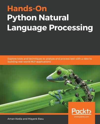
For the purposes of the chatbot that we will create in this section, we will be using Amazon's Q&A data, which is a repository of questions and answers gathered from Amazon's website for various product categories (http://jmcauley.ucsd.edu/data/amazon/qa/). Since the dataset is massive, we will only be using the Q&A data for electronic items. Being trained on Q&A data for electronic items, our chatbot could be deployed as automated Q&A support under the Electronic Items section. The following screenshot shows a partial snapshot of the corpus, which is in a JavaScript Object Notation (JSON)-like format:

As we can see, each row of data is in a dictionary format with various key-value pairs. Now that we have familiarized ourselves with the corpus, let's design the architecture of the chatbot, as follows:

1. Store all the questions from the corpus in a list
2. Store all corresponding answers from the corpus in a list
3. Vectorize and preprocess the question data
4. Vectorize and preprocess the user's query
5. Assess the most similar question to the user's query using cosine similarity
6. Return the corresponding answer to the most similar question as a chat response

Now that we have the blueprint of the solution, let's start coding. As the first step, we will need to import the corpus (qa_Electronics.json) into Python. We read the file as a text file and then use the ast library's literal_eval function to convert the rows from a string to a Python dictionary. We then iterate through each dictionary to extract and store questions and answers in separate lists, as shown in the following code block:

import ast 
questions = []
answers = [] 
with open('qa_Electronics.json','r') as f:
    for line in f:
        data = ast.literal_eval(line)
        questions.append(data['question'].lower())
        answers.append(data['answer'].lower())

While importing, we also perform the preprocessing step of converting all characters to lowercase. Next, using the CountVectorizer module of the sklearn library, we convert the questions list into a sparse matrix and apply TF-IDF transformation, as shown in the following code block:

from sklearn.feature_extraction.text import CountVectorizer
vectorizer = CountVectorizer(stop_words='english')
X_vec = vectorizer.fit_transform(questions)
tfidf = TfidfTransformer(norm='l2')
X_tfidf = tfidf.fit_transform(X_vec)

X_tfidf is the repository matrix that will be searched every time a new question is entered in the chatbot for the most similar question. To implement this, we create a function to calculate the angle between every row of the X_tfidfmatrix and the new question vector. We use the sklearn library's cosine_similarity module to calculate the cosine between each row and the vector, and then convert the cosine into degrees. Finally, we search the row that has the maximum cosine (or the minimum angle) with the new question vector and return the corresponding answer to that question as the response. If the smallest angle between the question vector and every row of the matrix is greater than a threshold value, then we consider that question to be different enough to not warrant a response. The implementation of the function is shown in the following code block:

def conversation(im):
    global tfidf, answers, X_tfidf
    Y_vec = vectorizer.transform(im)
    Y_tfidf = tfidf.fit_transform(Y_vec)
    angle = np.rad2deg(np.arccos(max(cosine_similarity(Y_tfidf, 
                       X_tfidf)[0])))
    if angle > 60 :
        return "sorry, I did not quite understand that"
    else:
        return answers[np.argmax(cosine_similarity(Y_tfidf, X_tfidf)[0])]

Lastly, we implement the chat, wherein the user enters their username and is then greeted by the chatbot. The chat is initiated with the user asking questions and the bot providing a response based on the preceding functions. The chat continues until the user typesbye. The implementation of the chat function is shown in the following code block:

def main():
    usr = input("Please enter your username: ")
    print("support: Hi, welcome to Q&A support. How can I help you?")
    while True:
        im = input("{}: ".format(usr))
        if im.lower() == 'bye':
            print("Q&A support: bye!")
            break
        else:
            print("Q&A support: "+conversation([im]))

That's it. We have just created a Q&A support chatbot that answers electronics products-related questions based on an existing repository of similar Q&As. The following is a sample conversation performed by the chatbot, which does not seem too bad for such a simple implementation:

Please enter your username: mike

support: Hi, welcome to Q&A support. How can I help you?

mike: what is the battery life of my phone?
Q&A support: so far after i charge the battery it will last about 90 minutes. i have not had any issues with the battery.

mike: great. does it have blue tooth?
Q&A support: no

mike: too bad. is there a replacement warranty on my phone?
Q&A support: the guarantee is one month. (the phone must be free of shocks or manipulated its hardware) the costs paid by the buyer.

mike: what about theft?
Q&A support: have to see if it covers it.

mike: bye
Q&A support: bye!

In this section, we used the concepts of vectorization and cosine similarity to create a basic chatbot. Needless to say, there is plenty of room for further improvement in this chatbot and we urge you to explore ways to improve its accuracy. Some areas that can be further refined are preprocessing, the cleaning of raw data, tweaking TF-IDF normalization, and so on. While cosine similarity-based chatbots were the first-generation NLP applications used in industry to automate simple Q&A-based tasks, new-age chatbots have come a long way and are able to handle much more complex and bespoke requirements using deep learning-based models. We will be covering some of these advanced concepts in the later chapters of this book.

Summary

In this chapter, we took baby steps in understanding the math involved in the representation of text data using numbers based on some heuristics. We made an attempt to understand the BoW model and build it using the CountVectorizer API provided by the sklearn module. After looking into limitations associated with CountVectorizer, we tried mitigating those using TfIdfVectorizer, which scales the weights of the less frequently occurring terms. We understood that these methods are purely based on lexical analysis and have limitations in terms of not taking into account features such as semantics associated with words, the co-occurrence of words together, and the position of words in a document, among others.

The study of the vectorization methods was followed up by making use of these vectors to find similarity or dissimilarity between documents using cosine similarity as the measure that provides the angle between two vectors in n-dimensional space. Finally, we looked into one-hot vectorization, a mechanism used for building vectors for tokens.

Which vectorization method to use where TD-IDF is concerned, of course, builds on top of the idea of CountVectorizer and helps in mitigating the issues involved with it. However, neither of these methods would scale well if the vocabulary is large or keeps on increasing. These would be ideally suited in use cases where the vocabulary size is limited and similar terms occur frequently across documents.

Now that we have understood a few mechanisms of representing text using its syntactical representation, let's take it forward in the next chapter by taking semantics into account as well. On these lines, let's explore techniques such as Word2vec in the next chapter.