In the previous chapter, we learned about advanced vector representation methodologies such as Doc2Vec and Sent2Vec, which significantly improve text processing accuracy. In this chapter, we will explore the applications of Machine Learning (ML) algorithms in Natural Language Processing (NLP). We will start with a gentle introduction to ML and learn about some additional preprocessing steps required for ML model training. We will then gain a thorough understanding of Naive Bayes and Support Vector Machine (SVM) algorithms and build a sentiment analyzer using them. By the end of this chapter, you will have gained a sound understanding of the application of ML algorithms for text processing and will be able to build a production-ready ML-based sentiment analyzer.

The following topics will be covered in this chapter:

• Introduction to ML
• Data preprocessing
• The Naive Bayes algorithm
• The SVM algorithm
• Productionizing a trained sentiment analyzer

Let's get started!

Technical requirements

The code files for this chapter can be found at the following GitHub link: https://github.com/PacktPublishing/Hands-On-Python-Natural-Language-Processing/tree/master/Chapter07.

Introduction to ML

ML is a subfield of artificial intelligence and aims at building systems that are capable of performing tasks without being explicitly programmed to do so. ML algorithms employ mathematical models that learn from existing data to perform tasks such as prediction, classification, decision-making, and so on. The learning bit of the model is also called training, where the model analyzes large volumes of data to identify patterns. This process is computationally intensive as the model needs to perform numerous calculations for the given data. However, with the continual advancement in computational power at our disposal, training, and the deployment of ML models, this has become fairly easy and quite popular. Since NLP also requires that we analyze large volumes of data, ML algorithms are widely applied in terms of text processing.

ML algorithms can be divided into three categories, as shown in the following diagram:

Let's look at these in more depth:

• Supervised learning: Supervised learning algorithms involve training the model using labeled data. The training dataset contains values of independent variables (also called a feature set) and the corresponding values of dependent variables. The algorithm analyzes these values and tries to learn a function that maps the independent variables to the dependent variables. Some widely used supervised learning algorithms include linear regression, k-nearest neighbor, decision tree, random forest, SVMs, Naive Bayes, and so on.
• Unsupervised learning: Unsupervised learning algorithms involve training the model using unlabeled data. The training process involves studying the dataset to understand the underlying structure of the data. Unsupervised learning is mostly used to cluster data and to perform anomaly detection by analyzing a data point with respect to other data points in the training set. Popular unsupervised algorithms include k-means, k-medoids, BIRCH, DBSCAN, and so on.

• Reinforcement learning: Reinforcement learning algorithms involve training the model based on simulations wherein the model learns based on the rewards that it receives for performing certain actions. Examples of popular reinforcement learning algorithms include Q-learning, SARSA, and so on.

While all three categories of ML algorithms have found applications in the field of text processing, NLP tools based on supervised learning algorithms are the most popular among the three categories. Supervised learning-based tools have a sizable adoption in the industry and they enjoy an established track record. Given their importance, we will delve into the nitty-gritty of two popularly used supervised learning algorithms. We will then combine our understanding of these algorithms with the tools we have learned so far to create and deploy a reasonably accurate NLP tool (sentiment analyzer).

Data preprocessing

Before we delve into these models and gain familiarity with some of these algorithms, we must learn about preprocessing the training data. We covered some of the preprocessing steps when working with text data such as tokenization, stop word removal, lemmatization, stemming, and so on in Chapter 3, Building Your NLP Vocabulary. However, there are some additional data preprocessing steps that are extremely crucial in ML as the training data needs to adhere to certain rules to be of any value to the model. Poorly processed data is guaranteed to train low accuracy models. It should be noted that data preprocessing is a vast field and that you may be required to perform various preprocessing steps based on the data you are working with. For example, you may be required to handle unstructured data; perform outlier analysis, invalid data analysis, and duplicate data analysis; identify correlated features; and more. However, we will focus on some of the most widely used preprocessing steps that are almost always required.

We will be performing preprocessing on the Tips dataset, which comes with the seaborn Python package. First, let's import the dataset and print out the first five lines to gain a basic understanding of the dataset:

import seaborn as sns

tips_df = sns.load_dataset('tips')
tips_df.head()

Here's the output:

  total_bill tip sex smoker day time size
0 16.99 1.01 Female No Sun Dinner 2
1 10.34 1.66 Male No Sun Dinner 3
2 21.01 3.50 Male No Sun Dinner 3
3 23.68 3.31 Male No Sun Dinner 2
4 24.59 3.61 Female No Sun Dinner 4

This dataset contains information about tips that have been paid in a particular restaurant by its patrons. Other than the tip amount, the dataset contains information regarding the total bill amount, the gender of the person paying the bill, the number of people in the group, the day and time of the visit, and whether there were any smokers in the group. Per the output, we can figure out that the sex, smoker, day, and time features are categorical features, whereas the others are numeric.

From the outset, we can see that there are some clear challenges with the data. Let's address them one by one.

NaN values

Data needs to be checked for NaN values after it's been imported. This is important because undetected NaN values can be very problematic for training and may even cause the training process to fail. Detecting NaN values is easy and can be done in various ways. The following is an example of how the pandas isnull() function can be used to figure out if there are any NaN values in the dataset:

tips_df.isnull().values.any()

The preceding command scans the entire dataset and returns True if there is even a single NaN in the dataset. The following is the output:

False

For this dataset, we do not have any NaN values. However, had the output been true, you would then be interested to determine which column or which row contains the NaN values. This can be done by running the following command:

tips_df.isnull().any()

This will output the result of the NaN search, which provides the results for each column, as follows:

total_bill False
tip False
sex False
smoker False
day False
time False
size False
dtype: bool

To identify the rows with NaN values, we need to pass the value 1 for the axis parameter of the any() function, which will scan the data for NaN values along the rows. The updated command is as follows:

tips_df.isnull().any(axis=1)

The following is the partial output of the preceding command, which shows the results of the search along the rows:

0 False
1 False
2 False
3 False
4 False
5 False
6 False
7 False

Once the NaN values have been identified, you need to decide what to do with them. Among the many methods for addressing NaN values, some of the popular methods are as follows:

• Dropping the row/column with NaN value(s). The dropna() function can be used to drop rows/columns containing NaN value(s).
• Replacing the NaN value with another value. The value could be the previous value, the next value, zero, the mean of the row or column, and so on. This can be done using the fillna() function.

There is no boilerplate solution to addressing NaN values, and how to deal with NaN values is a question that needs to be answered by the user.

Label encoding and one-hot encoding

In the Tips dataset, we can see that there are four categorical variables, namely sex, smoker, day, and time. The values of these variables are non-numeric, which is problematic because the mathematical models underpinning our ML system only understand numeric inputs. Therefore, we need to convert these non-numeric values into numeric values, which can be done by label encoding. As the name suggests, we use label encoding to map non-numeric values to numeric values.

To perform label encoding, we import the LabelEncoder class from sklearn's preprocessing module and apply the fit_transform() function to the non-numeric categorical variables of the DataFrame, as follows:

from sklearn.preprocessing import LabelEncoder
label_encoding = LabelEncoder()
tips_df.iloc[:,[2,3,4,5]] = tips_df.iloc[:,[2,3,4,5]].apply(label_encoding.fit_transform)

This transforms the tips_df DataFrame containing all the non-numeric categorical variables so that they're encoded as numeric variables, as shown in the following partial output of tips_df:

  total_bill  tip sex smoker day time size
0      16.99 1.01   0      0   2    0    2
1      10.34 1.66   1      0   2    0    3
2      21.01 3.50   1      0   2    0    3
3      23.68 3.31   1      0   2    0    2
4      24.59 3.61   0      0   2    0    4

To map non-numeric values to the encoded value, you can use the fit function on the relevant column and then print out the unique values for that column, as well as the corresponding encoding (using the transform() method), as follows:

label_encoding = LabelEncoder()
col_fit = label_encoding.fit(tips_df["day"])
dict(zip(col_fit.classes_, col_fit.transform(col_fit.classes_)))

The following is the output of the preceding code, along with the encoded values for the day column of the DataFrame:

{0: 0, 1: 1, 2: 2, 3: 3}

By using label encoding, we have addressed the issue of non-numeric data values in the dataset. However, encoding categorical variables that are nominal (where the values of the variable can't be ordered; for example, gender, days in a week, color, and so on) and not ordinal (the values of the variable can be ordered; for example, rank, size, and so on) creates another complication. For example, in the preceding case, we encoded Friday as 0 and Saturday as 1. When we feed these values to a mathematical model, it will consider these values as numbers and therefore will consider 1 to be greater than 0, which is not a correct treatment of these values.

To address this issue, we can use one-hot encoding, which splits a column with categorical variables into multiple columns, with each new column corresponding to a unique value of the categorical variable. In the preceding example, using one-hot encoding on the day column will result in four columns (Fri, Sat, Sun, Thur), with each column containing only 0 or 1, depending on whether the unique value occurred in a given row. We introduced one-hot encoding in the One-hot vectorization section in Chapter 4, Transforming Text into Data Structures, where we built a one-hot matrix for a corpus. We will now learn how to use sklearn's OneHotEncoder method to do the same. Please note that we will be applying one-hot encoding only after performing label encoding.

To perform one-hot encoding, we need to import the ColumnTransformer class from sklearn's compose module and the OneHotEncoder class from sklearn's preprocessing module. Since we are essentially transforming the columns of the DataFrame by splitting categorical features, we need to use this class. The OneHotEncoder class goes as an argument to the ColumnTransformer object which tells our program what kind of transformation we seek. We also need to pass the list of columns on which we seek to perform the transformation and use the remainder=passthrough argument to ignore other columns. Finally, just like label encoding, we'll apply the fit_transform() function to the DataFrame and store the output as an array called tips_df_ohe, as follows:

from sklearn.preprocessing import OneHotEncoder
from sklearn.compose import ColumnTransformer
oh_encoding = ColumnTransformer([('OneHotEncoding', OneHotEncoder(), 
                                [2,3,4,5])],remainder='passthrough')
tips_df_ohe = oh_encoding.fit_transform(tips_df)
tips_df_ohe

This splits all the labeled categorical variables in the tips_df DataFrame into columns for each unique value, as shown in the following output of tips_df_ohe:

array([[ 1. , 0. , 1. , ..., 16.99, 1.01, 2. ],
       [ 0. , 1. , 1. , ..., 10.34, 1.66, 3. ],
       [ 0. , 1. , 1. , ..., 21.01, 3.5 , 3. ],
       ...,
       [ 0. , 1. , 0. , ..., 22.67, 2. , 2. ],
       [ 0. , 1. , 1. , ..., 17.82, 1.75, 2. ],
       [ 1. , 0. , 1. , ..., 18.78, 3. , 2. ]])

There is still an outstanding issue that we need to resolve and that is the issue of the dummy variable trap. Say we use one-hot encoding on the day variable, which has four unique values. Splitting this variable into four columns will cause collinearity in our data (high correlation between variables) because we can always predict the outcome of the fourth column with the three other columns (if the day is not Friday, Saturday, or Sunday, then it will have to be Thursday). To address this issue, we will need to drop one dummy variable from the split columns of each categorical variable. This could be done by simply passing the argument drop='first' when defining the OneHotEncoder class.

Data standardization

Standardization is a data preprocessing step that attempts to equalize the range of values for all the columns. This is important because most ML algorithms require data to be in the same range, and non-uniform value ranges can impair the model's ability to learn from the data. For example, if all the columns in a dataset are in the range of [0, 10], whereas values in one column range from [-1000, 1000], then there is a high likelihood that this column will have a disproportionate influence over the model and that the trained model will be pretty much a one-to-one mapping between this column and the dependent variable. Therefore, you should always try to standardize the data before feeding it into the model for training. There are various standardization techniques we can use, but the two most popular techniques are min-max standardization and z-score standardization.

Min-max standardization

Each value in a column is transformed using the following formula:

Here, X is the vector representing the column. Each value in the column is subtracted by the minimum value of the column and divided by the column range. Post transformation, the range of the column becomes [0, 1].

Min-max standardization is quite simple to implement using the pandas min() and max() functions. However, since we have been discussing sklearn, here is how we can import the MinMaxScaler class from sklearn's preprocessing module to implement min-max standardization:

from sklearn.preprocessing import MinMaxScaler
minmax = MinMaxScaler()
tips_df_std = minmax.fit_transform(tips_df_ohe)
tips_df_std

The following is the output of the tips_df_std DataFrame. We can see that the one-hot encoded vectors remain the same, whereas other vectors are transformed so that they fit in the range [0, 1]:

array([[1. , 0. , 1. , ..., 0.29157939, 0.00111111, 0.2 ],
       [0. , 1. , 1. , ..., 0.1522832 , 0.07333333, 0.4 ],
       [0. , 1. , 1. , ..., 0.3757855 , 0.27777778, 0.4 ],
        ...,        
       [0. , 1. , 0. , ..., 0.41055718, 0.11111111, 0.2 ],
       [0. , 1. , 1. , ..., 0.30896523, 0.08333333, 0.2 ],
       [1. , 0. , 1. , ..., 0.32907415, 0.22222222, 0.2 ]])

Z-score standardization

Z-score standardization transforms the column by calculating the z-score for each value, as per the following formula:

Here, X is the vector representing the column. The z-score is the numerical measurement of how many standard deviations away a value from the mean of the group is. Post transformation, most values are expected to fall in the range of [-3, 3].

We can use the StandardScaler() class of sklearn's preprocessing module to implement z-score standardization, as shown here:

from sklearn.preprocessing import StandardScaler
zs = StandardScaler()
tips_df_std = zs.fit_transform(tips_df_ohe)
tips_df_std

The following is the output of the tips_df_std DataFrame. We can see that z-score standardization transforms each vector, depending on the mean and standard deviation:

array([[-0.06415003, -0.06415003, -0.09090909, ..., -0.42278122,
        -0.14463921, -0.12909944],
       [-0.06415003, -0.06415003, -0.09090909, ..., -0.42278122,
        -0.14463921, -0.12909944],
       [-0.06415003, -0.06415003, -0.09090909, ..., -0.42278122,
        -0.14463921, -0.12909944],
       ...,
       [-0.06415003, -0.06415003, -0.09090909, ..., -0.42278122,
        -0.14463921, -0.12909944],
       [-0.06415003, -0.06415003, -0.09090909, ..., -0.42278122,
        -0.14463921, -0.12909944],
       [-0.06415003, -0.06415003, -0.09090909, ..., -0.42278122,
        -0.14463921, -0.12909944]])

Now that we have covered various preprocessing techniques, we will explore some ML algorithms we can use to build NLP applications.

The Naive Bayes algorithm

In this section, we will delve into the Naive Bayes algorithm and build a sentiment analyzer. Naive Bayes is a popular ML algorithm based on the Bayes' theorem. The Bayes' theorem can be represented as follows:

Here, A, B are events:

• P(A|B) is the probability of A given B, while P(B|A) is the probability of B given A.
• P(A) is the independent probability of A, while P(B) is the independent probability of B.

Let's say we have the following fictitious dataset containing information about applications to Ivy League schools. The independent variables in the dataset are the applicant's SAT score, applicant's GPA, and information regarding whether the applicant's parents are alumni to an Ivy League school. The dependent variable is the outcome of the application. Based on this data, we are interested in calculating the likelihood of an applicant getting admission to an Ivy League school given that their SAT score is greater than 1,500, their GPA is greater than 3.2, and their parents are not alumni:

The likelihood of an applicant being admitted to an Ivy League school can be represented as a probability expression, as follows:

P(Ivy League|(SAT>1500, GPA>3.2, AP=0))

Using Bayes' theorem, the preceding probabilistic expression can be represented as follows:

We can solve the given equation by calculating the respective joint probabilities given in the previous table. However, for bigger datasets, calculating joint probability can get a bit challenging. To get around this problem, we use Naive Bayes, which assumes that all the features are independent of each other, so the joint probability is simply the product of independent probabilities. This assumption is naive because it is almost always wrong. Even in our example, an applicant having a high SAT score is more likely to have a high GPA, so these two events are not independent. However, the Naive Bayes assumption has been proved to work well for classification problems.

Using the Naive Bayes assumption we provided in the previous example, the Bayes' theorem expression can be written as follows:

This equation can easily be solved by calculating the respective probabilities. The numerator can be calculated as follows:

(2/4) * (2/4) * (1/4) * (4/7)

The denominator can be calculated as follows:

(2/7) * (5/7) * (4/7)

By calculating the ratio of the products, the final answer as 0.306, which can be rounded to 0. So, based on the data, Naive Bayes calculation predicts that an applicant with a SAT score > 1,500, GPA > 3.2, and parents not being alumni is not likely to be admitted to Ivy League. This is an unfair world!

Building a sentiment analyzer using the Naive Bayes algorithm

Sentiment analysis, sometimes called opinion mining or polarity detection, refers to the set of algorithms and techniques that are used to extract the polarity of a given document; that is, it determines whether the sentiment of a document is positive, negative, or neutral. Sentiment analysis is gaining popularity in the industry as it allows organizations to mine opinions of a large group of users or potential customers in a cost-efficient way. Sentiment analysis is now used extensively in advertisement campaigns, political campaigns, stock analysis, and more.

Now that we understand the mathematics behind the Naive Bayes algorithm, we will build a sentiment analyzer by training our Naive Bayes model on a labeled product review dataset gathered from Amazon. This dataset was created for the paper, From Group to Individual Labels using Deep Features, Kotzias et. al., KDD 2015, and can be accessed at http://archive.ics.uci.edu/ml/datasets/Sentiment+Labelled+Sentences.

The data is stored in a text file. The following is a partial snapshot of the text file:

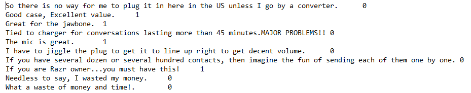
As we can see, the document contains a list of customer reviews and each review is assigned a sentiment score, with 0 representing negative sentiment and 1 representing positive sentiment.

First, we will import the raw data into a DataFrame called data, as follows:

import pandas as pd
data = pd.read_csv("amazon_cells_labelled.txt", sep='	', header=None)
data.head()

Here are the first five lines of the DataFrame:

0 So there is no way for me to plug it in here i... 0
1 Good case, Excellent value. 1
2 Great for the jawbone. 1
3 Tied to charger for conversations lasting more... 0
4 The mic is great. 1

Next, we will separate the columns that contain text reviews and the column containing sentiment labels:

X = data.iloc[:,0] # extract column with reviews
y = data.iloc[:,-1] # extract column with sentiments

We're doing this because the text data needs to be preprocessed for the ML model. Following this, we will import the CountVectorizer class, which performs key preprocessing steps on the text data such as tokenization, stop word removal, one-hot encoding, and so on. The following code snippet shows how CountVectorization is used to preprocess the text data:

from sklearn.feature_extraction.text import CountVectorizer
vectorizer = CountVectorizer(stop_words='english')
X_vec = vectorizer.fit_transform(X)
X_vec.todense() # convert sparse matrix into dense matrix

The following is the matrix, with each row representing a review and each column representing a unique word in the corpus. Each row vector represents the word count in that row for each unique word:

matrix([[0, 0, 0, ..., 0, 0, 0],
        [0, 0, 0, ..., 0, 0, 0],
        [0, 0, 0, ..., 0, 0, 0],
        ...,
        [0, 0, 0, ..., 0, 0, 0],
        [0, 0, 0, ..., 0, 0, 0],
        [0, 0, 0, ..., 0, 0, 0]], dtype=int64)

Next, we import the TfidfTransformer class to transform word counts into their respective tf-idf values (refer to Chapter 4, Transforming Text into Data Structures, for more details). Here is how we can transform the word count matrix into a matrix with corresponding tf-idf values:

from sklearn.feature_extraction.text import TfidfTransformer
tfidf = TfidfTransformer()
X_tfidf = tfidf.fit_transform(X_vec)
X_tfidf = X_tfidf.todense()

The following is the tf-idf matrix. Please note that because each review in the corpus is quite brief, the majority of the values in each row of the matrix are set to 0:

matrix([[0, 0, 0, ..., 0, 0, 0],
        [0, 0, 0, ..., 0, 0, 0],
        [0, 0, 0, ..., 0, 0, 0],
        ...,
        [0, 0, 0, ..., 0, 0, 0],
        [0, 0, 0, ..., 0, 0, 0],
        [0, 0, 0, ..., 0, 0, 0]], dtype=int64)

With this, we've completed the preprocessing part and are now ready to train the model using the processed data. However, before we do that, we need to split the data into training and testing sets so that we can evaluate the performance of our trained model. This is called cross-validation and is an important part of ML model training. We can easily split the data manually but for the sake of consistency, let's use the train_test_split class of sklearn's model_selection module to do this. For this, we pass our processed reviews data (X_tfidf) and the sentiment data to the train_test_split object and pass another argument regarding the desired ratio of the split, as follows:

from sklearn.model_selection import train_test_split
X_train, X_test, y_train, y_test = train_test_split(X_tfidf, y, test_size = 0.25, random_state = 0)

The preceding code splits both independent variables (the tfidf matrix) and the dependent variable (sentiment) into training and testing data.

We now have everything we need to train our model. For this, we need to import the MultinomialNaive Bayes class from sklearn's naive_bayes module and fit the training data to the model, as follows:

from sklearn.naive_bayes import MultinomialNaive Bayes
clf = MultinomialNaive Bayes()
clf.fit(X_train, y_train)

Fitting the training data essentially means that our Naive Bayes classifier has now learned the training data and is now in a position to calculate relevant probabilities. Therefore, if an out-of-sample review (such as I was very disappointed with this product) is now passed to the classifier, it will try to calculate the probability of the sentiment being positive or negative given that the words this, disappointed, and product exist in the review. Here is how we obtain the predicted sentiment values from the classifier for the test reviews that are stored in the y_pred array:

y_pred = clf.predict(X_test)

To determine the performance of our model, we will create a confusion matrix that calculates the number of correct predictions, broken down for each classification:

from sklearn.metrics import confusion_matrix
confusion_matrix(y_test, y_pred)

The following is the output of the confusion matrix. The vertical axis of sklearn's confusion matrix should be interpreted as the actual values, while the horizontal axis should be interpreted as the predicted values. Therefore, our model predicted 107 (87 + 20) values as having a sentiment score of 0, out which 87 were correctly predicted and 20 were incorrectly predicted. Likewise, the model predicted 143 (33+110) values as having a sentiment score of 1, out of which 110 were correctly predicted and 33 were incorrectly predicted:

array([[ 87, 33],
       [ 20, 110]], dtype=int64)

Therefore, the total number of correct predictions is obtained by summing the left diagonal (in this case, 87 + 110). The accuracy is the ratio of the total correct predictions divided by the total count of the test set (obtained by summing all the numbers in the confusion matrix). Therefore, the accuracy, in this case, is 197/250 = 78.8%. This is a decent accuracy score given the simple model and limited training data we had (only 750 abridged reviews). Tuning model parameters and performing further preprocessing steps such as lemmatization, stemming, and so on can improve the accuracy further.

The SVM algorithm

SVM is a supervised ML algorithm that attempts to classify data within a dataset by finding the optimal hyperplane that best segregates the classes. Each data point in the dataset can be considered a vector in an N-dimensional plane, with each dimension representing a feature of the data. SVM identifies the frontier data points (or points closest to the opposing class), also known as support vectors, and then attempts to find the boundary (also known as the hyperplane in the N-dimensional space) that is the farthest from the support vector of each class.

Say we have a fruit basket with two types of fruits in it and we want to create an algorithm that segregates them. We only have information about two features of the fruits; that is, their weight and radius. Therefore, we can abstract this problem as a linear algebra problem, with each fruit representing a vector in a two-dimensional space, as shown in the following diagram. In order to segregate the two types of fruit, we will have to identify a hyperplane (in two dimensions, the hyperplane would be a line) whose equation can be represented as follows:

Here, w1 and w2 are coefficients and c is a constant. The equation of the hyperplane in the n dimension can be generalized as follows:

Here, W is a vector of coefficients and X represents each dimension of the space.

From the preceding diagram, it is obvious that there are many hyperplanes that can segregate the two classes in this case. However, the SVM algorithm tries to find the optimum W (coefficients) and c (constant) so that the hyperplane is at the maximum distance from both support vectors. To perform this optimization, the algorithm starts with a hyperplane with random parameters and then calculates the distance of each point from the hyperplane using the following equation:

Knowing the distance of the hyperplane from each point, the algorithm can easily figure out the frontier points and calculate the distance from each support vector. The algorithm creates a number of hyperplanes and repeats this calculation to identify the hyperplane that's the most equidistant from both support vectors. This algorithm is also called linear SVM as the points are linearly separable. It should be noted that the SVM algorithm can also be applied to non-linearly separable data points, albeit after applying various transformations to the data.

Building a sentiment analyzer using SVM

In this section, we will build a sentiment analyzer using a linear SVM. We will be using the same dataset that we used to build the Naive Bayes-based sentiment analyzer for the sake of comparison. The feature matrix that was created while training the Naive Bayes sentiment analyzer had 1,642 columns, so the objective, in this case, is to identify a hyperplane that segregates vectors in a 1,642-dimensional space into positive sentiment classes and negative sentiment classes. This hyperplane will then be used to predict the sentiment of the newly vectorized and tf-idf transformed documents.

All the data preprocessing steps will be identical to those in the Naive Bayes sentiment analyzer section, as follows:

import pandas as pd
data = pd.read_csv("amazon_cells_labelled.txt", sep='	', header=None)

X = data.iloc[:,0] # extract column with review
y = data.iloc[:,-1] # extract column with sentiment

# tokenize the news text and convert data in matrix format
from sklearn.feature_extraction.text import CountVectorizer
vectorizer = CountVectorizer(stop_words='english')
X_vec = vectorizer.fit_transform(X)
X_vec = X_vec.todense() # convert sparse matrix into dense matrix

# Transform data by applying term frequency inverse document frequency (TF-IDF) 
from sklearn.feature_extraction.text import TfidfTransformer
tfidf = TfidfTransformer()
X_tfidf = tfidf.fit_transform(X_vec)
X_tfidf = X_tfidf.todense()

Again, we will split the processed input data into training data and testing data, as follows:

from sklearn.model_selection import train_test_split
X_train, X_test, y_train, y_test = train_test_split(X_tfidf, y, test_size = 0.25, random_state = 0)

The previous code splits both the independent variables (the tfidf matrix) and the dependent variable (sentiment) into training and testing data. Now, we import the Support Vector Classification (SVC) class from sklearn's svm module and fit the training data to the model, as follows:

from sklearn.svm import SVC
classifier = SVC(kernel='linear')
classifier.fit(X_train, y_train)

Fitting the training data means that the classifier has identified the optimum hyperplane after identifying the frontier points and calculating the relevant distances based on the training data. To assess the accuracy of the hyperplane, we will fit the vectorized test reviews (stored in the y_pred array) to the hyperplane equation. Based on the sign of the value of the equation, the model will predict the sentiment analysis score. The following command shows how the predicted values are calculated using the predict() function:

y_pred = classifier.predict(X_test)

Once again, we will be using a confusion matrix to measure the performance of our model, as follows:

from sklearn.metrics import confusion_matrix
confusion_matrix(y_test, y_pred)

Here is the output of the confusion matrix. Our model predicted 135 (102 + 33) values as having a sentiment score of 0, out which 102 were correctly predicted and 33 were incorrectly predicted. Likewise, the model predicted 115 (18+97) values as having a sentiment score of 1, out of which 97 were correctly predicted and 18 were incorrectly predicted:

array([[102, 18],
       [ 33, 97]], dtype=int64)

Therefore, the total number of correct predictions is obtained by summing the left diagonal (in this case, 102 + 97). The accuracy is the ratio of the total correct predictions divided by the total count of the test set (obtained by summing all the numbers in the confusion matrix). Therefore, the accuracy, in this case, 199/250 = 79.6%, which is marginally better than the Naive Bayes model's accuracy. The model's performance can be further improved by improving input data preprocessing (via lemmatization, stemming, and so on) and optimizing various SVM hyperparameters.

Productionizing a trained sentiment analyzer

Now that we have trained our sentiment analyzer, we need a way to reuse this model to predict the sentiment of new product reviews. Python provides a very convenient way for us to do this through the pickle module. Pickling in Python refers to serializing and deserializing Python object structures. In other words, by using the pickle module, we can save the Python objects that are created as part of model training for reuse. The following code snippet shows how easily the trained classifier model and the feature matrix, which are created as part of the training process, can be saved in your local machine:

import pickle
pickle.dump(vectorizer, open("vectorizer_sa", 'wb')) # Save vectorizer for reuse
pickle.dump(classifier, open("nb_sa", 'wb')) # Save classifier for reuse

Running the previous lines of code will save the Python object's vectorizer and classifier, which were created as part of the model training exercise we discussed in the Building a sentiment analyzer sections. These objects are saved as the vectorizer_sa and nb_sa files in your working directory. We can now import these pickled objects as we wish. We will use the same trained classifier and feature matrix as the ones we created during the training exercise.

Now, we will create a function that predicts the sentiment of any new product review. We will pass the trained classifier, feature matrix, and the new product review as parameters to this function and the function will return the predicted sentiment. The function simply vectorizes the new product review (passed as a string) based on the feature matrix that we have passed. The feature matrix is the matrix that contains all the words we learned from our training sample.

When we use the transform() function of the feature matrix on the new document, it simply creates a vector with the same number of elements as the number of columns (words) in the feature matrix and updates each element with the frequency of the corresponding word in the new document. The frequency vector is then transformed into a tf-idf vector before it's passed to the classifier. The function returns a positive or negative sentiment based on the classifier's output. Here is the implementation of the function:

def sentiment_pred(classifier, training_matrix, doc):
    """function to predict the sentiment of a product review

       classifier : pre trained model
       training_matrix : matrix of features associated with the trained 
       model
       doc = product review whose sentiment needs to be identified"""

    X_new = training_matrix.transform(pd.Series(doc)) 
    #don't use fit_transform here because the model is already fitted
    X_new = X_new.todense() #convert sparse matrix to dense

    from sklearn.feature_extraction.text import TfidfTransformer
    tfidf = TfidfTransformer()
    X_tfidf_new = tfidf.fit_transform(X_new)
    X_tfidf_new = X_tfidf_new.todense()

    y_new = classifier.predict(X_tfidf_new)
    if y_new[0] == 0:
        return "negative sentiment"
    elif y_new[0] == 1:
        return "positive sentiment"

Now that the function is ready, all we need to do is unpickle and import the classifier and feature matrix and pass them to the function, along with the new product review. The following code snippet shows how we can unpickle objects by using the load() function:

nb_clf = pickle.load(open("nb_sa", 'rb'))
vectorizer = pickle.load(open("vectorizer_sa", 'rb'))
new_doc = "The gadget works like a charm. Very satisfied with the product"
sentiment_pred(nb_clf, vectorizer, new_doc)

After this, we pass a fictitious product review to the function. The following is the output:

'positive sentiment'

Let's try passing another fictitious product review to our function:

new_doc = "Not even close to the quality one would expect"
sentiment_pred(nb_clf, vectorizer, new_doc)

Here is the output:

'negative sentiment'

As we can see, our ML-based sentiment analyzer is live and performing decently.

However, the following are some important things to consider while creating and deploying the sentiment analyzer:

• The training data should be consistent with the objective of the sentiment analyzer. Don't train the model using movie reviews if the objective is to predict the sentiment of financial news articles.
• Accurately labeling the training data is critical for the model to perform well. We have used pre-labeled data in this chapter. However, if you are creating a real-world application, you will have to spend time labeling the training documents. Typically, labeling should be done by someone with a good understanding of industry jargon.
• Sourcing training data is a difficult task. You can use tools such as web scraping or social media scraping, subject to permissions. Effort should be spent on sourcing data from multiple platforms and you shouldn't rely too much on a particular source.
• Evaluate the performance of your model regularly and retrain the model if required.

With that, we have come to the end of this chapter!

Summary

In this chapter, we built on our understanding of text vectorization, data preprocessing, and so on to gain an end-to-end understanding of applying ML algorithms to develop NLP applications. We learned about the additional pre-processing steps required for ML training and gained a thorough understanding of the Naive Bayes and SVM algorithms. We applied our understanding of text data processing and ML algorithms to build a sentiment analyzer and deployed the model to perform sentiment analysis in real-time. We also learned how to measure the performance of ML models and discussed some important dos and don'ts about building ML-based applications.

In the next chapter, we will learn how to apply deep learning to text processing and cover how neural networks can help us improve the accuracy of our applications.