Search in book...
Toggle Font Controls
Create new playlist

Name your new playlist

Playlist description (optional)
Sign In

Email address

Password

Forgot Password?

or

Continue with Facebook

Continue with Google
Sign Up

Full Name

Email address

Confirm Email Address

Password

or

Continue with Facebook

Continue with Google

Chapter 3

Aerodynamic Heating

Heat Transfer at High Speeds

Abstract

A physical description of aerodynamic heating is presented. The theory is presented for a flat plate boundary layer flow, and important parameters such as adiabatic wall temperature and recovery factor are introduced. A method to calculate the heat flux is outlined. A simple illustrative numerical example is described. An engineering practical system is analyzed.

Keywords

Adiabatic wall temperature; Boundary layer; Heat reduction; Recovery factor; Thermal protection

3.1. Introduction

In many engineering applications, it may be assumed that the influence on the energy balance by the work of the viscous forces is negligible. As the flow velocity becomes sufficiently high, this assumption will not be valid but instead the so-called frictional or viscous heating needs to be considered. Aerodynamic heating increases with the speed of the vehicle and it produces much less heat at subsonic speeds but becomes more significant at supersonic speeds. Aerodynamic heating is a concern for supersonic and hypersonic aircraft, as well as for reentry vehicles. The heating induced by the very high speeds greatly affects the overall design of aerospace vehicles. In addition the temperature gradients then become so large that the temperature dependence of the thermophysical properties also has to be considered. A thermal balance of aerodynamic heat input and thermal radiation heat loss to the sky for a flight at Ma = 4 at stratospheric altitudes results in an equilibrium surface temperature of about 800 C, which can be withstood by some steel materials. On the other hand, at hypersonic Mach numbers, there may be localized temperatures exceeding the melting temperatures of all substances. It can be estimated that for reentry vehicles the air temperature in the boundary layer may reach values above 5000 C. For hypersonic vehicles, it is generally known that aerodynamic heating is the dominant issue of the vehicle design. The heating effect is greatest at the leading edges and is dealt with by using high-temperature metal alloys, insulating the exterior of the vehicle, or using ablative materials.

The phenomenon of aerodynamic heating is, as stated earlier, of relevance and importance for aircraft, space vehicles, and missiles operating at supersonic velocity. Analysis of this type of problem is complicated. The purpose of this chapter is to introduce the phenomenon and present solutions for an idealized case. In many engineering cases involving high flow velocities along a flat plate and constant wall temperature, the wall heat flux can be calculated by the heat transfer coefficient, h, for the low-velocity case multiplied by the temperature difference, T_w−T_aw, where T_w is the wall temperature and T_aw is the so-called adiabatic wall temperature. The theory and background will be summarized. Examples are provided to illustrate the phenomenon.

3.2. High Velocity Flow Along a Flat Plate

Consider the high-speed motion of an incompressible fluid along a flat plate as depicted in Fig. 3.1.

The fluid is assumed to have constant thermophysical properties. According to Appendix 1, the laminar boundary layer equations read as follows:

Mass

$\frac{\partial u}{\partial x} + \frac{\partial v}{\partial y} = 0$ $\frac{\partial u}{\partial x} + \frac{\partial v}{\partial y} = 0$

(3.1)

Momentum

$u \frac{\partial u}{\partial x} + v \frac{\partial u}{\partial y} = v \frac{\partial^{2} u}{\partial y^{2}}$ $u \frac{\partial u}{\partial x} + v \frac{\partial u}{\partial y} = v \frac{\partial^{2} u}{\partial y^{2}}$

(3.2)

Energy

$u \frac{\partial T}{\partial x} + v \frac{\partial T}{\partial y} = α \frac{\partial^{2} T}{\partial y^{2}} + \frac{μ}{ρ c_{p}} {(\frac{\partial u}{\partial y})}^{2}$ $u \frac{\partial T}{\partial x} + v \frac{\partial T}{\partial y} = α \frac{\partial^{2} T}{\partial y^{2}} + \frac{μ}{ρ c_{p}} {(\frac{\partial u}{\partial y})}^{2}$

(3.3)

The last term in Eq. (3.3) represents the work by the viscous forces or the so-called frictional or viscous heating.

The boundary conditions of Eqs. (3.1)–(3.3) read

$y = 0 : u = v = 0, T = T_{w}$ $y = 0 : u = v = 0, T = T_{w}$

(3.4)

$y \to \infty : u \to U_{\infty}, T \to T_{\infty}$ $y \to \infty : u \to U_{\infty}, T \to T_{\infty}$

(3.5)

Figure 3.1 Boundary layer flow along a flat plate surface.

The flow field is not changed when compared to the low-speed case. The solution can be found in most heat transfer text books like Refs. [1,2].

The solution of the temperature field is split into two: a homogeneous solution and a particular solution. The homogeneous solution is obtained when the frictional heating term in Eq. (3.3) is neglected. The homogeneous solution of Eq. (3.3) can be written as

$T^{(h)} = T_{\infty} + (T_{w} - T_{\infty}) θ (η)$ $T^{(h)} = T_{\infty} + (T_{w} - T_{\infty}) θ (η)$

(3.6)

where the dimensionless coordinate η is given by,

η = \sqrt{\frac{U_{\infty}}{2 vx}} y .

$η = \sqrt{\frac{U_{\infty}}{2 vx}} y .$

As a particular solution of Eq. (3.3), one looks for the solution being valid for an adiabatic plate, i.e., q_w=0. With η defined as earlier and the approach of the concept of the stream function ψ (u = ∂ψ/∂y, v = −∂ψ/∂x, f′ = u/U_∞) is represented as

$ψ = \sqrt{{2 vU}_{\infty} x} f (η)$ $ψ = \sqrt{{2 vU}_{\infty} x} f (η)$

Eq. (3.3) can then be written as

$\frac{d^{2} T}{{dη}^{2}} + \Pr f \frac{dT}{dη} + 2 \frac{U_{\infty}^{2}}{2 c_{p}} \Pr f^{″ 2} = 0$ $\frac{d^{2} T}{{dη}^{2}} + \Pr f \frac{dT}{dη} + 2 \frac{U_{\infty}^{2}}{2 c_{p}} \Pr f^{″ 2} = 0$

(3.7)

The boundary conditions of Eq. (3.7) are

$η = 0 : \frac{dT}{dη} = 0 (q_{w} = 0)$ $η = 0 : \frac{dT}{dη} = 0 (q_{w} = 0)$

$η \to \infty : T \to T_{\infty}$ $η \to \infty : T \to T_{\infty}$

A dimensionless temperature θ^a is defined in Eq. (3.8)

$θ^{a} = \frac{T - T_{\infty}}{U_{\infty}^{2} / {2 c}_{p}}$ $θ^{a} = \frac{T - T_{\infty}}{U_{\infty}^{2} / {2 c}_{p}}$

(3.8)

By introducing θ^a in Eq. (3.7), one obtains

$\frac{d^{2} θ^{a}}{{dη}^{2}} + \Pr f \frac{{dθ}^{a}}{dη} + 2 Pr f^{″ 2} = 0$ $\frac{d^{2} θ^{a}}{{dη}^{2}} + \Pr f \frac{{dθ}^{a}}{dη} + 2 Pr f^{″ 2} = 0$

(3.9)

The boundary conditions are transferred as

$η = 0 : \frac{{dθ}^{a}}{dη} = 0$ $η = 0 : \frac{{dθ}^{a}}{dη} = 0$

(3.10)

$η \to \infty : θ^{a} \to 0$ $η \to \infty : θ^{a} \to 0$

(3.11)

Eq. (3.9) with the boundary conditions in Eqs (3.10) and (3.11) was solved by Eckert [5] many years ago. It was shown that the difference between the adiabatic wall temperature (the plate temperature for q_w=0) and the fluid temperature could be written as

$T_{aw} - T_{\infty} = r \cdot \frac{U_{\infty}^{2}}{2 c_{p}} = θ^{a} (0) \frac{U_{\infty}^{2}}{2 c_{p}}$ $T_{aw} - T_{\infty} = r \cdot \frac{U_{\infty}^{2}}{2 c_{p}} = θ^{a} (0) \frac{U_{\infty}^{2}}{2 c_{p}}$

(3.12)

where r is the so-called recovery factor, which depends on the Pr number of the fluid.

For moderate Pr numbers (e.g., gases, water) the recovery factor becomes

$r ≅ \sqrt{\Pr} for 0.6 < \Pr < 15$ $r ≅ \sqrt{\Pr} for 0.6 < \Pr < 15$

(3.13)

The solution of Eq. (3.3) with the conditions Eqs. (3.4) and (3.5) is obtained by combining the homogeneous and the particular solutions, i.e.,

${T = T}^{(h)} {+ T}^{(p)}$ ${T = T}^{(h)} {+ T}^{(p)}$

${T = C}_{1} T_{\infty} + C_{2} (T_{w} - T_{\infty}) θ (η) + θ^{a} \frac{U_{\infty}^{2}}{2 c_{p}} + T_{\infty}$ ${T = C}_{1} T_{\infty} + C_{2} (T_{w} - T_{\infty}) θ (η) + θ^{a} \frac{U_{\infty}^{2}}{2 c_{p}} + T_{\infty}$

The boundary condition Eq. (3.5) requires C₁ = 0, whereas the boundary condition Eq. (3.4) implies

$T_{w} {= C}_{2} {(T}_{w} - T_{\infty}) \cdot 1 + (T_{aw} - T_{\infty}) + T_{\infty}$ $T_{w} {= C}_{2} {(T}_{w} - T_{\infty}) \cdot 1 + (T_{aw} - T_{\infty}) + T_{\infty}$

The constant C₂ is found from this expression as

$C_{2} = \frac{T_{w} - T_{aw}}{T_{w} - T_{\infty}}$ $C_{2} = \frac{T_{w} - T_{aw}}{T_{w} - T_{\infty}}$

The solution of Eq. (3.3) can therefore be written as

$T - T_{\infty} = (T_{w} - T_{aw}) θ (η) + θ^{a} \frac{U_{\infty}^{2}}{{2 c}_{p}}$ $T - T_{\infty} = (T_{w} - T_{aw}) θ (η) + θ^{a} \frac{U_{\infty}^{2}}{{2 c}_{p}}$

(3.14)

3.3. Calculation of the Heat Transfer

The heat flux from the plate surface q_w is written as usual, i.e.,

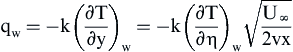
$q_{w} = - k {(\frac{\partial T}{\partial y})}_{w} = - k {(\frac{\partial T}{\partial η})}_{w} \sqrt{\frac{U_{\infty}}{2 vx}}$ $q_{w} = - k {(\frac{\partial T}{\partial y})}_{w} = - k {(\frac{\partial T}{\partial η})}_{w} \sqrt{\frac{U_{\infty}}{2 vx}}$

From Eq. (3.14), one finds

${(\frac{\partial T}{\partial η})}_{w} = (T_{w} - T_{aw}) {(\frac{\partial θ}{\partial η})}_{w} + {(\frac{\partial θ^{a}}{\partial η})}_{w} \frac{U_{\infty}^{2}}{{2 c}_{p}}$ ${(\frac{\partial T}{\partial η})}_{w} = (T_{w} - T_{aw}) {(\frac{\partial θ}{\partial η})}_{w} + {(\frac{\partial θ^{a}}{\partial η})}_{w} \frac{U_{\infty}^{2}}{{2 c}_{p}}$

However,

{(\frac{\partial θ^{a}}{\partial η})}_{w} = 0

${(\frac{\partial θ^{a}}{\partial η})}_{w} = 0$

and

{(\frac{\partial θ}{\partial η})}_{w}

${(\frac{\partial θ}{\partial η})}_{w}$

are the temperature derivatives for the low-speed case. From Ref. [1], the solution for the low-speed case can be found as

${(\frac{\partial θ}{\partial η})}_{w} = - \sqrt{2} \frac{h}{k} \sqrt{\frac{vx}{U_{\infty}}}$ ${(\frac{\partial θ}{\partial η})}_{w} = - \sqrt{2} \frac{h}{k} \sqrt{\frac{vx}{U_{\infty}}}$

The heat flux can now be written as

$q_{w} = h (T_{w} - T_{aw})$ $q_{w} = h (T_{w} - T_{aw})$

(3.15)

Thus a simple method to calculate the heat flux at high flow velocities has been found.

The heat transfer coefficient for the corresponding low-speed case is multiplied by the temperature difference, T_w−T_aw, where T_aw is the so-called adiabatic wall temperature. This temperature is determined using the recovery factor r (Eq. (3.12).

3.4. Turbulent Flow

The described analysis is valid for laminar boundary layers. For a turbulent boundary layer, it has been found that the heat flux at high velocities can be calculated similarly. Turbulent flow prevails where Re_x = U_∞ x/v > 5·10⁵. The recovery factor is determined by Ref. [4]

$r = \Pr^{1 / 3}$ $r = \Pr^{1 / 3}$

(3.16)

The heat transfer coefficient for turbulent low flow velocities can be found in most heat transfer text books, e.g., Refs. [1,2].

3.5. Influence of the Temperature Dependence of the Thermophysical Properties

In Section 3.1, it was mentioned that at high flow velocities the thermophysical properties will be affected because of the large temperature gradients. This means that these properties may vary considerably across the boundary layer. A complete analysis is too extensive but Pohlhausen [3] recommends that the thermophysical properties are evaluated at a reference temperature T∗ according to

${T∗ = T}_{\infty} + 0.5 (T_{w} - T_{\infty}) + 0.22 (T_{aw} - T_{\infty})$ ${T∗ = T}_{\infty} + 0.5 (T_{w} - T_{\infty}) + 0.22 (T_{aw} - T_{\infty})$

(3.17)

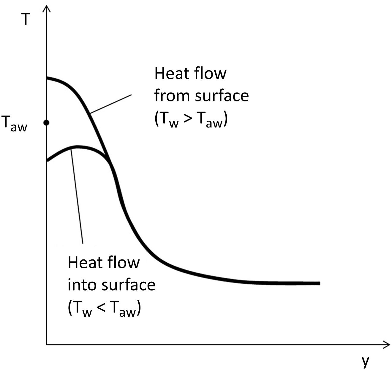
3.6. Temperature Distribution in the Boundary Layer

Fig. 3.2 presents a temperature profile in the thermal boundary on a flat surface. If the wall temperature is higher than the adiabatic wall temperature, heat is transferred from the surface to the gas. On the other hand, if the wall temperature is below the adiabatic wall temperature, heat is transferred from the fluid to the surface.

3.7. Illustrative Example

Consider a flat plate, as in Fig. 3.1, with the dimensions, length, 70 cm and width, 1 m. The plate is placed in a wind tunnel where the flow conditions are given by Ma = 3, p = 0.05 atm, temperature −40°C. Two tasks are described in the following: (1) to calculate the recovery temperature and (2) to calculate the cooling rate to maintain the plate surface temperature at 35°C.

1. The freestream sound velocity, a, is first calculated as

$a = \sqrt{γRT} = {(1.4 \cdot 287 \cdot 233)}^{1 / 2} = 306 m/s$ $a = \sqrt{γRT} = {(1.4 \cdot 287 \cdot 233)}^{1 / 2} = 306 m/s$

Figure 3.2 Temperature distribution in a boundary layer along a flat plate.

Then the freestream velocity is

$U_{\infty} = 3 \cdot 306 = 918 m/s$ $U_{\infty} = 3 \cdot 306 = 918 m/s$

The maximum Reynolds number is estimated using the properties at the freestream conditions:

$ρ_{\infty} = p/RT = 0.0758 {kg/m}^{3}, μ_{\infty} = 1.434 \cdot 10^{- 5} kg/ms; {Re}_{L} = ρ_{\infty} U_{\infty} L / μ_{\infty} = 3.395 \cdot 10^{6}$ $ρ_{\infty} = p/RT = 0.0758 {kg/m}^{3}, μ_{\infty} = 1.434 \cdot 10^{- 5} kg/ms; {Re}_{L} = ρ_{\infty} U_{\infty} L / μ_{\infty} = 3.395 \cdot 10^{6}$

Thus one needs to consider both the laminar and the turbulent boundary layers.

Laminar boundary layer: With Pr = 0.7 the recovery factor becomes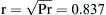

r = \sqrt{Pr} = 0.837

$r = \sqrt{Pr} = 0.837$

. From Eq. (3.12), one obtains T_aw = −40 + 0.837·918²/(2·1005) = 311°C.

Now the thermophysical properties should be recalculated based on the reference temperature in Eq. (3.17). However, it is found that the differences are small.

Turbulent boundary layer: According to Eq. (3.16) the recovery factor becomes r = 0.7^1/3 = 0.888.

The corresponding adiabatic wall temperature is found to be T_aw = −40 + 0.888·918²/(2·1005) = 332°C.

2. The cooling rate can be calculated as follows

$Q_{w} = h \cdot A \cdot (T_{aw} - T_{\infty})$ $Q_{w} = h \cdot A \cdot (T_{aw} - T_{\infty})$

The low-speed heat transfer coefficient needs to be found for the laminar and the turbulent boundary layers. By using the critical Reynolds number for transition as 5·10⁵, it can be found that the length of the laminar boundary layer is 0.222 m and that of the turbulent boundary layer is 0.478 m.

Laminar boundary layer: The average heat transfer coefficient can be found from Ref. [1]

Nu = {hL}_{lam} / k = 0.664 \cdot \sqrt{Re \cdot {Pr}^{1 / 3}}

$Nu = {hL}_{lam} / k = 0.664 \cdot \sqrt{Re \cdot {Pr}^{1 / 3}}$

, which gives h_lam = 56.3 W/m²K. Then the heat flow rate is Q_lam = 56.3·(0.222·1)·(311−35) = 3445 W.

Turbulent boundary layer: The corresponding heat transfer coefficient can be found from the local one given by Ref. [1],

Nu = h \cdot x / k = 0.0296 {Re}_{x}^{0.8} \cdot \Pr^{1 / 3}

$Nu = h \cdot x / k = 0.0296 {Re}_{x}^{0.8} \cdot \Pr^{1 / 3}$

. However, the average value has to be found by averaging from x = 0.222 m to x = 0.7 m. The average value becomes h_turb = 87.5 W/m²K. Then the heat flow rate is Q_turb = 87.5·(0.47·1)·(332−35) = 12,415 W.

The total amount of heat to be cooled from the plate becomes

$Q_{tot} = Q_{lam} + Q_{turb} = 15860 W .$ $Q_{tot} = Q_{lam} + Q_{turb} = 15860 W .$

3.8. An Engineering Example of a Thermal Protection System

As mentioned in Section 3.1, space vehicles have to withstand extremely high aerodynamic heating and pressure loads during the ascent and reentry stages. The primary function of a thermal protection system (TPS) is to keep the underlying structure within acceptable temperature limits and to maintain the aerodynamic shape of the vehicle without excessive deformation (thermal bowing and bending caused by pressure loads). A TPS must provide thermal protection and also have structural load bearing capabilities and be robust, durable, and easily maintained. Although satisfying all these requirements, the weight of the TPS must be as low as possible to keep the launch costs low. A sandwich panel to be used as a TPS is shown in Fig. 3.3. Significant efforts have been taken toward the development of integrated thermal protection system (ITPS) that exhibits the function of thermal protection and load-bearing capabilities [6–10].

The objective of this example is to present findings from an investigation [11] that developed an analytical procedure to optimize and obtain a minimum-mass corrugated-core sandwich panel to function as an ITPS for space vehicles. The optimal dimensions for both thermal and structural constraints were attempted, but the two constraints were not active at the same instant of time. Accordingly the optimization problem was solved in two steps. In the first step, the design process for the corrugated-core ITPS was initiated by a transient thermal analysis to obtain the temperature distribution as a constraint and load. Seven dimensions of the unit cell were considered as the geometric design variables. The thickness of the insulation was optimized in the thermal sizing study, and then the optimal height of the core was determined. In the second step, the geometry of the ITPS panel was optimized, except for the height of the core identified in the first step. The structural sizing optimization considered both thermal and mechanical loads. The globally convergent method of moving asymptotes (GCMMA) [12] was used as the optimization algorithm. The ANSYS Parametric Design Language (APDL) code was developed to analyze the thermomechanical coupling model.

Figure 3.3 A typical corrugated-core sandwich structure for thermal protection system (TPS), with top face sheet, web, and bottom faceplates.

3.8.1. Thermal Analysis

Consider a simplified geometry of an ITPS unit cell as shown in Fig. 3.4. The unit cell consists of two inclined webs and two thin faceplates. The top faceplate thickness, t_TF, may be different from the bottom faceplate thickness, t_BF, as well as the web thickness t_W. The unit cell is identified by seven geometric parameters (p, d, t_TF, t_BF, t_W, θ, and l). The thickness of the insulation is the only concern. The top and bottom faceplate thicknesses are constant because they have limited effect on the maximum temperature of the internal structure. The temperature on the top surface of the ITPS panel is always close to the radiation equilibrium temperature. It is controlled by the emissivity of the top surface, which typically has a value in the range of 0.8–0.85 [13]. Increasing the emissivity is not a design issue but is related to manufacturing and material selection. The thermal load and boundary conditions imposed on the two-dimensional (2D) model are shown in Fig. 3.5.

Furthermore, the following assumptions are made:

1. No temperature variation in the direction along the outer surface of the panel.

Figure 3.4 A simplified geometry of an ITPS unit cell: two inclined webs with the thickness t_W and two thin faceplates with the thickness t_TF and t_BF.

Figure 3.5 Loading and boundary conditions for a simplified ITPS structure model: instantaneous heat flux and radiation are assigned on the outer faceplate, whereas inner face sheet is perfectly insulated.

2. The lower surface of the bottom faceplate is assumed to be perfectly insulated. Optimization with this assumption leads to a conservative design.

3. Radiation is applied on the upper surface of the top faceplate, with an emissivity of 0.85.

4. Initial temperature of the model is assumed to be constant.

5. Radiative and convective heat transfer through the insulation material is ignored, and only the conductive heat transfer is taken into account.

3.8.2. Finite Element Analysis of Heat Transfer

The material thermal properties will change with temperature and pressure and accordingly the heat transfer problem turns into a nonlinear transient problem, which is relatively complicated. According to these assumptions, the governing heat conduction equation can be expressed as follows [1]:

$ρc \frac{\partial T}{\partial τ} = \frac{\partial}{\partial x} (k \frac{\partial T}{\partial x})$ $ρc \frac{\partial T}{\partial τ} = \frac{\partial}{\partial x} (k \frac{\partial T}{\partial x})$

(3.18)

where ρ, k, and c is the density, thermal conductivity, and specific heat of the insulation material, respectively; τ is the time; and T is the temperature.

By discretization of Eq. (3.18), the finite element equation in the heat transfer analysis is transformed to the general form:

$[C (T)] [T^{'}] + [K_{c} (T)] [T] = [Q (T)]$ $[C (T)] [T^{'}] + [K_{c} (T)] [T] = [Q (T)]$

(3.19)

where C is the specific heat matrix; K_c, conductivity matrix; Q, nodal heat flow vector; and T and

T^{'}

$T^{'}$

, the nodal temperature vector and the derivative of the nodal temperature versus time, respectively. Each nodal transient temperature can be obtained using the Newmark method combined with the Newton–Raphson method to solve Eq. (3.19).

The thermal boundary conditions are as follows. The considered aerodynamic heat flux is under the assumption of laminar flow and is imposed on the upper surface of the top faceplate during reentry. The ambient temperature and initial structural temperature are both assumed to be 273 K. A large portion of heat is radiated out to the ambient by the upper surface of the top faceplate. The net thermal radiation is determined by

$q_{r} {= ε}_{s} σ_{s} (T_{t}^{4} - T_{\infty}^{4})$ $q_{r} {= ε}_{s} σ_{s} (T_{t}^{4} - T_{\infty}^{4})$

(3.20)

where q_r is the radiative heat flux; ε_s, the surface emissivity; σ_s, the Stefan–Boltzmann constant; T_t, the top faceplate temperature; and T_∞, ambient temperature.

After the vehicle has touched down, it is cooled only by natural convection. During this period, the temperature of the bottom faceplate rises to a maximum value. In this case, a convective heat transfer boundary condition is imposed on the upper surface of the top faceplate instead of radiation, as shown by Eq. (3.21):

$q_{c} {= h (T}_{t} - T_{\infty})$ $q_{c} {= h (T}_{t} - T_{\infty})$

(3.21)

where q_c is the convective heat flux; h, the convective heat transfer coefficient; T_t, the top faceplate temperature; and T_∞, the ambient temperature. Here, the value of the convective coefficient, h, was assumed to be 6.5 W/m²K [10].

In the transient thermal analysis, thermal properties, which may be a function of temperature and pressure, are updated at each time step. The aerodynamic pressure load on the vehicle during reentry is presented in Fig. 3.6 [6]. Based on the material properties database, the transient heat transfer analysis is divided into four load steps to fit the pressure profile.

The aerodynamic heating and natural convection coefficient profiles are presented in Fig. 3.7.

3.8.3. Thermal Results

In the studied case, a material combination based on Ref. [10] was selected. The materials from the top faceplate to the bottom faceplate are as follows: aluminosilicate/Nextel 720 composites (for top faceplate and web), Saffil insulation, and epoxy/carbon fiber laminate (for bottom faceplate). The material properties are taken from Refs [10] and [15] and are listed in Table 3.1.

Figure 3.6 The aerodynamic pressure load on the vehicle during reentry: the instantaneous aerodynamic pressure is approximated by multiple-line variations. The pressure data was adapted from Grujicic M, Zhao CL, Biggers SB, Kennedy JM, Morgan DR. Heat transfer and effective thermal conductivity analyses in carbon-based foams for use in thermal protection systems. Proceedings of the Institution of Mechanical Engineers, Part L: Journal of materials: design and applications, 219(4):217–230; Martinez OA, Sankar BV, Haftka RT, Blosser ML. Two-dimensional orthotropic plate analysis for an integral thermal protection system, AIAA J 2012; vol. 50, pp. 387–398.

Figure 3.7 The aerodynamic heating and natural convection coefficient profiles: an instantaneous heat flux is imposed up to about 2300 s, whereas only constant natural convection is imposed beyond 2300 s.

Fig. 3.8 presents temperature variations versus reentry times for some featured points. It shows that the top faceplate reaches its peak temperature after 1500 s. When the aerodynamic convection-based input heat flux is balanced by the emitted radiative heat flux, the temperature of the top faceplate becomes equal to the radiation equilibrium temperature, which is determined by a given input heat flux and a given surface emissivity. The variations of the temperature along the thickness direction of the ITPS at several selected time steps are provided in Fig. 3.9. The temperature gradients of the structure at each characteristic time step are provided. At about 6350 s, the structure will not be heated any more, as the temperature gradient approaches zero.

A structural finite element model was used to calculate the stress of the top faceplate and the web. An assumed uniform pressure loading of 5000 Pa was applied on the sandwich outer surface, and temperatures are applied over the entire model, as illustrated in Fig. 3.10. The peak radiation equilibrium temperature for the reentry heat flux is 990 °C at 1500 s [15]. Therefore the temperature distribution at 1500 s is chosen to simulate the situation where the thermal stress caused by the thermal gradient reaches its maximum value. In this calculation, the height of the sandwich core was fixed. The insulation material was not considered to be a structural member because the Saffil insulation is a soft fibrous insulation material with hardly any mechanical properties, but it was also modeled to simulate more realistic thermal expansion environment for the sandwich panel. In addition, temperature-dependent properties are ignored to further simplify the model and the material properties are considered to have fixed values.

Table 3.1

Material Thermo Physical Properties

	Materials
	Aluminosilicate-Nextel 720 Fiber Composite	Epoxy/carbon Fiber Laminate	Saffil
Properties
Density, ρ (kg/m³)	2450–2600	1550–1580	50
Young's modulus, E (GPa)	133.5–139.1	49.7–60.1	＼
Compressive strength, σ_bc (MPa)	67.9–68.8	542.1–656.8	＼
Tensile strength, σ_bt (MPa)	67.9–68.8	248.6–355.9	＼
Poisson's ratio, μ	0.23–0.25	0.305–0.307	＼
Specific heat, c (J/kgK)	950–1100	901.7–1037	942–1340
Thermal conductivity, k (W/mK)	2.52–2.93	1.28–2.6	0.052–0.5
Thermal expansion, α (10⁻⁶/K)	5.745	0.36–4.02	＼

Figure 3.8 Variations in temperature with the reentry time for the featured points (distance from bottom: 0, 30, 60, 90, and 134 mm).

Figure 3.9 Temperature profiles in the thickness direction of the ITPS at several selected time steps: 500, 1500, 2500, 4000, and 6350 s.

Figure 3.10 Mechanical and thermal loads on the panel during reentry of the vehicle: a uniform pressure of 5000 Pa and temperature from the heat transfer analysis were applied on the top faceplate.

The maximum von Mises stress of the ITPS unit cell occurs at four constraint points and is far less than the yielding strength of the epoxy/carbon fiber laminate. The maximum von Mises stress of the top faceplate and webs occurs at the edge of the webs.

Further details of this example of engineering relevance can be found in Ref. [16].

3.9. Aerodynamic Heat Reduction

In Section 3.7 a TPS was analyzed. However, there are several studies concerning reduction of the aerodynamic heating by using active techniques such as an opposing jet, a forward-facing spike, or an opposing jet from an extended nozzle, as illustrated in Fig. 3.11. As the heat transfer mechanism in high enthalpy flow (supersonic and cold hypersonic flows) is different from that in low enthalpy flow, the design of a TPS is affected accordingly. As the flow speed exceeds the Mach number of unity, a shock wave is formed in front of the body and the flow temperature rises as it passes through it. As the temperature rises above a certain value, molecules in the air dissociate and become radicals. The radicals recombine on the body surface and then the surface is heated by radiation. The recombination rate on the surface depends on the catalysity of the surface. In turn the catalysity depends on the surface temperature and the substance of the surface. Accordingly the flow phenomena become complex by dissociation and recombination, but these processes reduce the flow temperature because of the loss of energy caused by dissociation. There is then a possibility that the aerodynamic heating is reduced by cutting down the convective heat transfer and the radiation heat transfer. It is known that oxygen and nitrogen molecules begin dissociation at a temperature of 2500 K and 4000 K, respectively. Thus for air, effects of dissociation and recombination have to be considered when the temperature backward of the shock reaches these temperatures.

Figure 3.11 Conjectured flow pattern for active TPS by opposing jets. (a) opposing jet, (b) spike, and (c) opposing jet from extended nozzle.

Application of an opposing jet is a method to cool body surfaces in supersonic and hypersonic flows by injecting a coolant gas forward. Accordingly, many experimental investigations and CFD simulations have been applied in analyzing such systems to reduce the aerodynamic heating (as well as drag). It has been found that a strong opposing jet flow and a long extended nozzle reduce the aerodynamic heating and drag significantly. The opposing jet covers the body surface with the coolant gas and insulates the surface from the high-temperature gas, thus reducing the convective heat transfer. The radiative heat transfer is reduced by preventing recombination of the dissociated gas on the body surface. An additional cooling effect might be obtained close to the injection location because this region is protected by the jet and the recirculating flow. Relevant research works are described in Refs. [17–19].

..................Content has been hidden....................

You can't read the all page of ebook, please click here login for view all page.

Table of Contents for Chapter 3. Aerodynamic Heating: Heat Transfer at High Speeds

Create new playlist

Sign In

Sign Up