
Case study
Image clustering
Abstract
The bag-of-words (BoW) model is one of the most popular approaches to image classification and forms an important component of image search systems. The BoW model treats an image’s features as words, and represents the image as a vector of the occurrence counts of image features (words). This chapter discusses the OpenCL implementation of an important component of the BoW model—namely, the histogram builder. We discuss the OpenCL kernel, and study the performance impact of various source code optimizations.
The bag-of-words (BoW) model is one of the most popular approaches to image classification and forms an important component of image search systems. The BoW model treats an image’s features as words, and represents the image as a vector of the occurrence counts of image features (words). This chapter discusses the OpenCL implementation of an important component of the BoW model—namely, the histogram builder. We discuss the OpenCL kernel and study the performance impact of various source code optimizations.
9.1 Introduction
Image classification refers to a process in computer vision that can classify an image according to its visual content. For example, an image classification algorithm may be designed to tell if an image contains a human figure or not. While detecting an object is trivial for humans, robust image classification is still a challenge in computer vision applications.
The BoW model is a commonly used method in document classification and natural language processing. In the BoW model, the frequency of the occurrence of each word in the document is used as a parameter for training a machine learning algorithm. In addition to document classification, the BoW model can also be applied to image classification. To apply the BoW model to classify images, we need to extract a set of words (just like in document classification) from the image and count their occurrence. In computer vision, the words extracted from an image are commonly known as features. A feature generation algorithm reduces an image to a set of features that can serve as a signature for an image. A high-level algorithm for image classification is shown in Figure 9.1, and consists of feature generation, clustering, and histogram building steps, which are briefly described below:
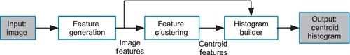
1. Feature generation: The feature generation algorithm we have applied in the BoW model is the speeded up robust features (SURF) algorithm. SURF was first introduced in 2006 by Bay et al. [1], and is a popular algorithm that is invariant to various image transformations. Given an input image, the SURF algorithm returns a list of features illustrated in Figure 9.2. Each feature includes a location in the image and a descriptor vector. The descriptor vector (also referred to as a descriptor) is a 64-dimension vector for each feature. The descriptor contains information about the local color gradients around the feature’s location. In the context of this chapter, feature refers to the 64 element descriptor which is a part of each feature. The remainder of this chapter does not focus on the location information generated as part of the feature.

2. Image clustering: The descriptors generated from the SURF algorithm are usually quantized, typically by k-means clustering, and mapped into clusters. The centroid of each cluster is also known as a visual word.
3. Histogram builder: The goal of this stage is to convert a list of SURF descriptors into a histogram of visual words (centroids). To do this, we need to determine to which centroid each descriptor belongs. In this case, both the descriptors of the SURF features and the centroid have 64 dimensions. We compute the Euclidean distance between the descriptor and all the centroids, and then assign each SURF descriptor to its closest centroid. The histogram is formed by counting the number of SURF descriptors assigned to each centroid.
Using this approach, we can represent images by histograms of the frequency of the centroids (visual words) in a manner similar to document classification. Machine learning algorithms such as a support vector machine can then be used for classification. A diagram of this execution pipeline is shown in Figure 9.1.
In this chapter, we explore the parallelization of the histogram-building stage in Figure 9.1. We first introduce the sequential central processing unit (CPU) implementation and its parallelized version using OpenMP. Then we move to multiple parallel implementations using OpenCL that are targeted toward a graphics processing unit (GPU) architecture. Several implementations are discussed, including a naive implementation, a version that uses more optimal accesses to global memory, and additional versions that utilize local memory. At the end of the chapter, an evaluation of performance is provided using an AMD Radeon HD 7970 GPU.
9.2 The Feature Histogram on the CPU
In this section, we first introduce the algorithm for converting SURF features into a histogram and implement a sequential version for execution on a CPU. We then parallelize the algorithm using OpenMP to target a multicore CPU.
9.2.1 Sequential Implementation
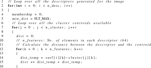
Listing 9.1 shows the procedure for converting the array of SURF features into a histogram of cluster centroids (visual words). Line 3 loops through the SURF descriptors and line 8 loops through the cluster centroids. Line 13 loops through the 64 elements of the current descriptor to compute the Euclidean distance between the SURF feature and the cluster centroid. Line 19 finds the closest cluster centroid for the SURF descriptor and assigns its membership to the cluster.
9.2.2 OpenMP parallelization
To take advantage of the cores present on a multicore CPU, we use OpenMP to parallelize Listing 9.1. The OpenMP application programming interface supports multiplatform shared-memory parallel programming in C/C++ and Fortran. It defines a portable, scalable model with a simple and flexible interface for developing parallel applications on platforms from desktops to supercomputers [2]. In C/C++, OpenMP uses pragmas (#pragma) to direct the compiler on how to generate the parallel implementation.
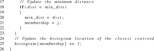
Using OpenMP, we can distribute the histogram-building step across the multiple CPU cores by dividing the task of processing SURF descriptors between multiple threads. Each thread computes the distance from its descriptor to the cluster centroids and assigns membership to a centroid. Although the computation for each descriptor can be done independently, assigning membership to the histogram creates a race condition: if multiple threads try to update the same location simultaneously, the results will be undefined. This race condition can be solved by using an atomic addition operation (line 26). The histogram algorithm using OpenMP parallelization is showing in Listing 9.2.
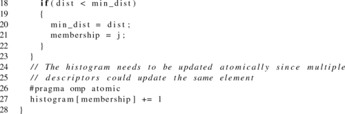
In Listing 9.2, the pragma on line 3 is used to create threads and divide the loop iterations among them. The pragma on line 19 tells the compiler to use an atomic operation when updating the shared memory location.
9.3 OpenCL Implementation
In this section, we discuss the OpenCL implementation of the histogram builder. We first implement a naive OpenCL kernel based on the sequential and OpenMP versions of the algorithm. Then we explain how this naive implementation can be improved for execution on GPUs by applying optimizations such as coalesced memory accesses and using local memory.
9.3.1 Naive GPU Implementation: GPU1
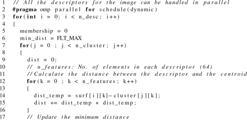
Given the parallel algorithm shown in Listing 9.2, the simplest way to parallelize the algorithm in OpenCL would be to decompose the computation across the outermost loop iterations: where each OpenCL work-item is responsible for computing the membership of a single descriptor.
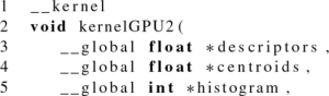
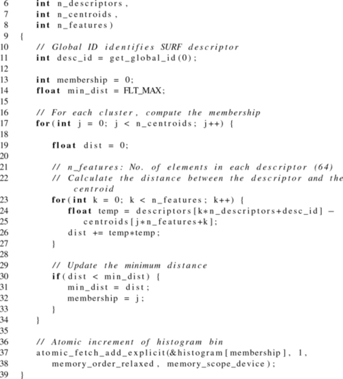
However, as with the OpenMP example, this implementation creates a race condition as multiple work-items update the histogram in global memory. To solve this issue, we use an atomic addition to update the histogram as we did for the OpenMP parallelization. The code for this naive OpenCL kernel is shown in Listing 9.3. We refer to this implementation as GPU1.
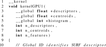
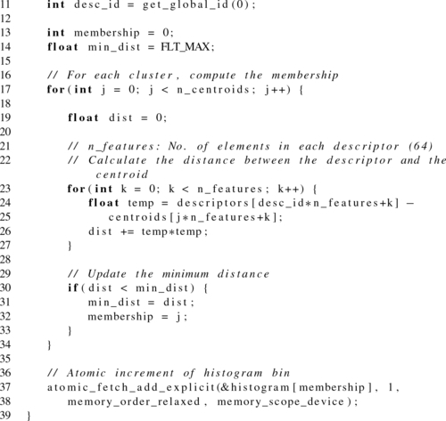
Notice that in Listing 9.3, the atomic increment on line 38 is performed using a relaxed memory order. We chose this option because we are performing only a simple counter update, so enforcing stronger ordering requirements is not needed. See Chapter 7 for more details.
9.3.2 Coalesced Memory Accesses: GPU2
Recall that successive work-items are executed in lockstep when running on GPU single instruction, multiple data (SIMD) hardware. Also recall that SURF descriptors and cluster centroids comprise vectors of 64 consecutive elements. Keeping this information in mind, take a look at line 25 of Listing 9.3, and notice the access to descriptors. Given what we know about GPU hardware, would line 25 result in high-performance access to memory?
Suppose there are four work-items running in parallel with global IDs ranging from 0 to 3. When looping over the features in the innermost loop, these four work-items would be accessing memory at a large stride—in this kernel, the stride will be n_features elements. Assuming that we are processing centroid 0 (j = 0), when computing the distance for feature 0 (k = 0), the work-items would produce accesses to descriptors[0], descriptors[64], descriptors[128], and descriptors[192]. Computing the distance for the next feature would generate accesses to descriptors[1], descriptors[65], descriptors[129], and descriptors[193], and so on.
Recall from Chapter 8 that accesses to consecutive elements can be coalesced into fewer requests to the memory system for higher performance, but that strided accesses generate multiple requests, resulting in lower performance. This strided pattern when accessing the buffers is uncoalesced and suboptimal.
To improve the memory bandwidth utilization by increasing the memory coalescing, we need to adjust the order in which elements are stored in the descriptors buffer. This can be done by using a data layout transformation known as a transpose, which is demonstrated in Figure 9.3. In a transpose, the rows and column positions of each element are exchanged. That is, for an element Ai,j in the original matrix, the corresponding element in the transposed matrix is Aj,i. We create a simple transformation kernel where each thread reads one element of the input matrix from global memory and writes back the same element at its transposed index in the global memory.
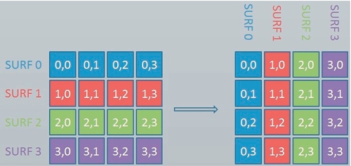
Since we are using a one-dimensional array for the input buffers, an illustration of applying a transpose kernel is shown in Figure 9.4. After the transformation, descriptors[0], descriptors[64], descriptors[128], and descriptors[192] are stored in four consecutive words in memory and can be accessed by four work-items using only one memory transaction.

After the transformation, line 25 of Listing 9.4 shows that descriptors is now indexed by k*n_descriptors+desc_id. As k and n_descriptors have the same value for all work-items executing in lockstep, the work-item accesses will be differentiated solely by their ID (desc_id). In our previous example of four work-items, k = 0 would produce accesses to descriptors[0], descriptors[1], descriptors[2], and descriptors[3]. When k = 1, accesses would be generated for descriptors[64], descriptors[65], descriptors[66], and descriptors[67]. This access pattern is much more favorable, and allows GPU coalescing hardware to generate highly efficient accesses to the memory system.
9.3.3 Vectorizing Computation: GPU3
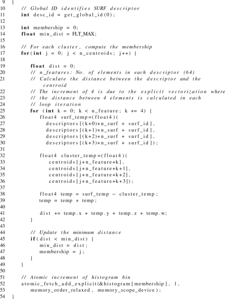
Since each SURF descriptor is a fixed-sized vector with 64 dimensions, vectorization with float4 has the ability to substantially increase the utilization of the processing elements. This type of vectorization on a CPU would allow the compiler to take advantage of Streaming SIMD Extensions instructions for higher-throughput execution. Some families of GPUs (e.g. AMD Radeon 6xxx series) could also take advantage of vectorized operations. Newer GPUs from AMD and NVIDIA do not explicitly execute vector instructions; however, in some scenarios this optimization could lead to high performance from improved memory system utilization or improved code generation.
Vectorization can allow us to generalize operations on scalars transparently to vectors, matrices, and higher-dimensional arrays. This can be done explicitly by the developer in OpenCL using the float4 type. The listing below is an explicit vectorization of the addition operations in the listing above.
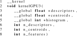
To introduce vectorization into our algorithm, the OpenCL kernel is updated as shown in Listing 9.5, named as implementation GPU3.
9.3.4 Move SURF Features to Local Memory: GPU4
The following snippet shows the memory accesses to descriptors and centroids from Listing 9.4:
Notice that the data in both of these buffers is accessed multiple times. Is it possible to take advantage of one of the other OpenCL memory spaces to improve performance? When centroids are accessed, the address used to index the buffer is independent of the work-item’s ID. This type of access pattern is favorable for constant memory, which we will discuss in the next iteration of the algorithm. For this version, we will focus on optimizing accesses to descriptors. Since addressing descriptors is dependent on the work-item ID, it is not well suited for constant memory. However, can we take advantage of local memory instead?
Recall that when running applications on most GPUs, local memory is a high-bandwidth, low-latency memory used for sharing data among work-items within a work-group. On GPUs with dedicated local memory, access to local memory is usually much faster than accesses to global memory. Also, unlike accesses to global memory, accesses to local memory usually do not require coalescing, and are more forgiving than global memory when having nonideal access patterns (such as patterns that cause large numbers of memory bank conflicts). However, local memory has limited size—on the AMD Radeon HD 7970 GPU there is 64 KB of local memory per compute unit, with the maximum allocation for a single work-group limited to 32 KB. Allocating large amounts of local memory per work-group has the consequence of limiting the number of in-flight threads. On a GPU, this can reduce the scheduler’s ability to hide latency, and potentially leave execution resources vacant.
Initially, this data does not seem to be a good candidate for local memory, as local memory is primarily intended to allow communication of data between work-items, and no data is shared when accessing descriptors. However, for some GPUs such as the Radeon HD 7970, local memory has additional advantages. First, local memory is mapped to the local data store (LDS), which provides four times more storage than the general-purpose level 1 (L1) cache. Therefore, placing this buffer in the LDS may provide low-latency access to data that could otherwise result in cache misses. The second benefit is that even assuming a cache hit, LDS memory has a lower latency than the L1 cache. Therefore, with enough reuse, data resident in the LDS could provide a speedup over the L1 cache even with a high hit rate. The trade-off, of course, is that the use of local memory will limit the number of in-flight work-groups, potentially underutilizing the GPU’s execution units and memory system. This is an optimization that needs to be considered on a per-architecture basis. A version of the kernel utilizing local memory to cache descriptors is shown in Listing 9.6.
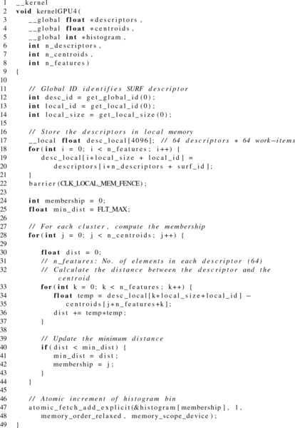
When descriptors are accessed, n_descriptors and desc_id are fixed per work-item for the entire duration of the kernel. The index simply varies on the basis of k. Therefore, each work-item will access the n_feature elements (64) of descriptors a total of n_centroids times (the j iterator). Given the small L1 cache sizes on GPUs, it is very likely that many of these accesses will generate L1 cache misses and cause redundant accesses to global memory.
Moving descriptors to LDS would require 64 × 4 = 256 bytes per descriptor. With a wavefront size of 64 work-items, each wavefront requires 16 KB of LDS to cache its portion of descriptors. This would allow at most four work-groups to be executed at a time per compute unit (one wavefront per work-group). On the Radeon HD 7970, each compute unit comprises four SIMD units, limiting our execution to one work-group per SIMD unit and removing the ability to hide latency on a given SIMD unit. Any benefit we see from performance will be a trade-off between lower-latency memory accesses and decreased parallelism. We refer to this implementation as GPU4.
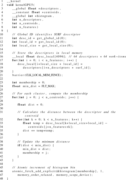
9.3.5 Move Cluster Centroids to Constant Memory: GPU5
As shown in the convolution example in Chapter 4, and the memory model discussion in Chapter 7, constant memory is a memory space that it intended to hold data that is accessed simultaneously by all work-items. Data typically stored in constant memory would include convolution filters and constant variables such as π. In the case of our histogram kernel, the descriptors for each centroid also fit this characteristic. Notice that when centroids are accessed, the address depends on two of the loop iterators, but never on the work-item ID. Therefore, work-items executing in lockstep will generate identical addresses.
The trade-off for mapping centroids to constant memory is that on GPUs constant memory usually maps to specialized caching hardware that is a fixed size. In the case of the Radeon HD 7970, the largest buffer size that can be mapped to constant memory is 64 KB. For this example, the features for each centroid consume 256 bytes. Therefore, we can map at most 256 centroids at a time to constant memory.
Alert readers may also question the effectiveness of mapping centroids to constant memory. If all work-items are accessing the same address, will not the accesses be coalesced and generate only a single request to global memory? On most modern GPUs, the answer is yes: only a single request will be generated. However, similarly to mapping descriptors to LDS, there are additional benefits to mapping centroids to constant memory. The first benefit of utilizing constant memory is to remove pressure from the GPU’s L1 cache. With the small L1 cache capacity, removing up to 64 KB of recurring accesses could lead to a significant performance improvement. The second benefit is that the GPU’s constant cache also has a much lower latency than does accessing the general-purpose L1 cache. As long as our data set has few enough centroids to fit into constant memory, this will likely lead to a significant performance improvement.
Mapping the centroids buffer to constant memory is as simple as changing the parameter declaration from __global to __constant, as shown in Listing 9.7.
9.4 Performance Analysis
To illustrate the performance impact of the various kernel implementations, we executed the kernels on a Radeon HD 7970 GPU. To additionally provide insight into the impact of data sizes on the optimization, we generated inputs with various combinations of SURF descriptors and cluster centroids. We varied the number of SURF descriptors between 4096, 16,384, and 65,536. At the same time, we varied the number of cluster centroids between 16, 64, and 256. We picked large numbers of SURF features because a comprehensive high-resolution images can usually contains thousands of features. However, for cluster centroids, the numbers are relatively small since a large number of clusters could reduce the accuracy of image classification.
The performance experiments described in this section can be carried out using performance profiling tools such as AMD’s CodeXL, which is described in detail in Chapter 10. The performance discussed in this chapter is used only for illustrating the benefits of source code optimization of OpenCL kernels. The performance impact of each optimization will vary depending on the targeted architecture.
9.4.1 GPU Performance
We evaluate performance, and keep in mind that GPU1 requires only a single OpenCL kernel. However, the rest of the implementations require a transpose kernel to be called before execution of the histogram kernel, and thus consist of two kernels. The transpose kernel overhead is based solely on the number of SURF descriptors, and will not be impacted by other changes. Therefore, we separate out the transpose timing in Table 9.1, so that the impact from the other performance results can be viewed in isolation. The execution time for the second kernel from each implementation is shown in Table 9.2.
Table 9.1
The Time Taken for the Transpose Kernel
| No. of Features | Transform Kernel (ms) |
| 4096 | 0.05 |
| 16,384 | 0.50 |
| 65,536 | 2.14 |
All implementations other than GPU1 execute this kernel. To make an accurate comparison between GPU1 and all other kernels, these values should be added to the execution time of the histogram kernel (shown in Table 9.2).
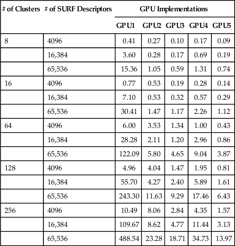
Table 9.2
Kernel Running Time (ms) for Different GPU Implementations
| # of Clusters | # of SURF Descriptors | GPU Implementations | ||||
| GPU1 | GPU2 | GPU3 | GPU4 | GPU5 | ||
| 8 | 4096 | 0.41 | 0.27 | 0.10 | 0.17 | 0.09 |
| 16,384 | 3.60 | 0.28 | 0.17 | 0.69 | 0.19 | |
| 65,536 | 15.36 | 1.05 | 0.59 | 1.31 | 0.74 | |
| 16 | 4096 | 0.77 | 0.53 | 0.19 | 0.28 | 0.14 |
| 16,384 | 7.10 | 0.53 | 0.32 | 0.57 | 0.29 | |
| 65,536 | 30.41 | 1.47 | 1.17 | 2.26 | 1.12 | |
| 64 | 4096 | 6.00 | 3.53 | 1.34 | 1.00 | 0.43 |
| 16,384 | 28.28 | 2.11 | 1.20 | 2.96 | 0.86 | |
| 65,536 | 122.09 | 5.80 | 4.65 | 9.04 | 3.87 | |
| 128 | 4096 | 4.96 | 4.04 | 1.47 | 1.95 | 0.81 |
| 16,384 | 55.70 | 4.27 | 2.40 | 5.89 | 1.61 | |
| 65,536 | 243.30 | 11.63 | 9.29 | 17.46 | 6.43 | |
| 256 | 4096 | 10.49 | 8.06 | 2.84 | 4.35 | 1.57 |
| 16,384 | 109.67 | 8.62 | 4.77 | 11.44 | 3.13 | |
| 65,536 | 488.54 | 23.28 | 18.71 | 34.73 | 13.97 | |
9.5 Conclusion
In this chapter, we performed various source code optimizations on a real-world OpenCL kernel. These optimizations included improving memory accesses using a data transformation, implementing vectorized mathematical operations, and mapping data to local and constant memory for improved performance. We evaluated the implementations on a GPU to observe the performance impact of each optimization.