4

MISCONCEPTION 3: Spending More on R&D Increases Innovation

It seems almost obvious that increasing R&D investment will increase innovation. In fact, this belief is so widely held that when the government wanted to increase innovation in 1981, it implemented R&D tax credits. The government’s goal for innovation is similar to companies’ goal. Both want growth. Companies want growth because it increases their market value; the government wants economic growth because it increases the number of jobs, the level of wages, and accordingly the standard of living for all its citizens. What’s convenient about economic growth is that it’s largely just the collective growth of all the companies in the economy. So the best way for the government to achieve its growth goal is to help companies achieve their growth goals.

THE THEORY LINKING R&D TO GROWTH

The intuition that technological innovation leads to growth has existed since at least Adam Smith’s Wealth of Nations.¹ So it is interesting that the formal theory linking R&D to growth is fairly recent. That theory, called endogenous growth theory, was introduced in a 1990 paper by the economist Paul Romer.² The foundation of that theory is the production function, which links inputs (typically capital and labor) to output. The first extension of the production function linking it to innovation came from another economist, however. Robert Solow, in 1957, observed that U.S. output was growing faster than what you would expect from the growth in capital and labor. He concluded that there must be a missing input. He called this missing input “technological change.”³ Technological change essentially increases the amount of output from any given level of other inputs. A simple example of a technology increasing the output of employees is personal computers. PCs makes employees more efficient (except of course when they’re using them for leisure, such as ordering gifts on Cyber Monday).

Solow’s observation of substantial growth from technological change begs the question of where that technological change comes from. This is where Solow and Romer differ. Solow believes that it occurs “exogenously,” meaning outside the productive activity of companies. In this view, knowledge essentially advances on its own, and companies get to take advantage of that advancing knowledge for free. In contrast, Romer believes that technological change comes from purposeful investment in R&D. In Romer’s theory, R&D activity combines with existing knowledge to create new knowledge. This new knowledge then combines with capital and labor to make them more productive. While Romer was working at the level of the economy, more recent theory has translated his theory into company-level versions that generate similar predictions for growth.⁴

The powerful benefit of having a formal theory (rather than merely intuition) is that it generates predictions you can test empirically. Testing these predictions allows researchers to determine if the theory is valid. What’s exciting about the predictions from endogenous growth theory is that they include an expectation that the economy will grow even in the absence of population growth, so long as there continues to be investment in R&D. Moreover, the theory makes a very specific prediction that the rate of growth is determined by the number of scientists and engineers doing R&D. In particular, the theory holds that doubling R&D labor will double the growth rate of the economy, a prediction called “scale effects.”

THE GROWTH PUZZLE

Here’s the puzzle: R&D labor has increased 250 percent since 1971, yet GDP growth has at best remained stagnant over the same period. In fact, a better characterization is that GDP growth has actually declined 0.03 percent per year! The fact that one of Romer’s predictions doesn’t hold up suggests Romer’s theory might be wrong.

Chad Jones, the economist who first documented the failure of the “scale effects” prediction in 1995, suggested the problem was that R&D has gotten harder, and Romer’s theory doesn’t account for that.⁵ Jones proposed that two mechanisms contributed to this. The first mechanism is something he called the “fishing out effect.” This is the notion that all the good ideas have already been cherry-picked. If you think about recent innovations such as personal computers, the Internet, and smartphones, you might be skeptical about this idea, but we’ll examine it more concretely in a moment. The second mechanism is “diminishing returns to R&D labor,” which is the notion that adding more scientists leads to substantial duplication of effort. Both of these ideas seem plausible. In fact, Robert Gordon, in The Rise and Fall of American Growth, makes similar arguments.⁶ The dismal outcome if Chad Jones and Robert Gordon are correct is that growth will decline to zero (other than for population growth).

I have a more optimistic explanation, which is that companies have gotten worse at R&D. While companies getting worse may not sound more optimistic than R&D getting harder, if it’s true, then we return to Romer’s world of perpetual growth as long as there continues to be R&D. Since Romer’s theory has been extended to the level of the company, this means not only will the economy continue to grow but companies should continue to grow as well. Moreover, if firms restore their prior level of R&D productivity, they should return to their prior levels of growth.

The big question now is whether Chad Jones and Robert Gordon are correct that R&D has gotten harder, or I’m correct that companies have gotten worse at it. We already saw in Chapter 1 that, on average, companies’ RQs have declined 65 percent. This suggests I’m right that companies have gotten worse. However, it will also look like companies have gotten worse if in fact R&D has gotten harder.

So we need a different test of whether R&D has gotten harder. You need to think outside the box to come up with such a test, but one thought is that if R&D has truly gotten harder, it should have gotten harder for everyone. In other words, not only will average RQ decrease each year, but maximum RQ will decrease as well. Thus if I take the best company in each year (the one with the highest RQ) and compare it to the best company the following year, then the later companies will tend to have lower RQs than earlier companies.

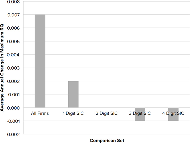
That’s not what I found when I examined 40 years of data. I found instead that maximum RQ was increasing over time! When you think about all the marvelous companies that have been created as part of the Internet economy, that seems plausible, but there is still reason to be skeptical when you’re swimming against the tide. Next, I checked whether the same pattern held if, instead of looking at all public companies, I restricted attention to a particular sector, such as manufacturing or services. I found that maximum RQ was increasing within sectors as well. I then looked at coarse definitions of industry using the U.S. Department of Labor’s Standard Industrial Classification (SIC) codes, such as Measuring Equipment (SIC 38), then successively more narrow definitions, such as Surgical, Medical, and Dental Instruments (SIC 384), then Dental Equipment (SIC 3843). What I found was that as I looked more narrowly, maximum RQ was decreasing over time (Figure 4-1). Thus Chad Jones’s theory might hold at the industry level. Within a given industry, R&D does appear to be getting harder over time. However, what’s exciting is that as some industries are dying off, companies are creating new industries with more technological opportunity. So overall, R&D appears to be getting easier rather than harder! It is easy to think of relevant examples: brick-and-mortar retail is dying, but Internet retail sales are growing; landlines are dying, but smartphone innovation seems to know no bounds.

To summarize where this leaves us with respect to endogenous growth theory, it appears that Romer’s theory is left intact. While his scale effects prediction doesn’t appear to hold (GDP growth is stagnant despite substantial increases in R&D labor), this seems to be due to a decline in companies’ R&D productivity (companies getting worse) rather than from a decline in technological opportunity (R&D getting harder). The encouraging implication from this is that companies and the economy should be able to grow in perpetuity as long as companies continue to conduct R&D. The less encouraging implication is that this won’t happen if RQ continues to decline. The challenge then is to determine why companies have gotten worse. If we understand that, then there’s hope they can regain their prior RQ, and accordingly restore their higher prior growth. If enough companies do that, then the economy should also return to the pre-1970 growth levels that Gordon hails in his book.

Now that I’ve introduced some new theory, it’s of course time for a test. What do you think happened when the U.S. government introduced R&D tax credits as part of the Economic Recovery Tax Act of 1981? In answering the question, it may be helpful to remember that the goal of the act was to reverse the dramatic decline in companies’ R&D investment that began in 1964. The hope was that restoring R&D investment would revive economic growth and bolster U.S. competitiveness against the then rising threat from Japanese manufacturing. Accordingly, this is a two-part question: (1) Did R&D tax credits restore R&D investment? and (2) Did the tax credits revive economic growth?

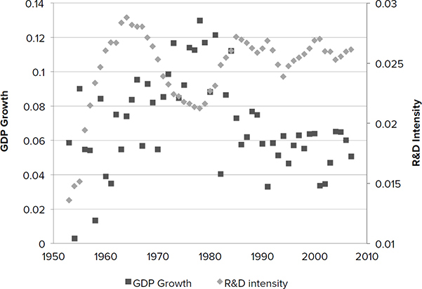
Now for the answers. The answer to question 1 is that the tax credits were extremely effective in increasing R&D. Within four years of implementation, R&D investment (plotted as diamonds in Figure 4-2) was restored to within 10 percent of its 1964 peak (2.9 percent of sales). However, the answer to question 2 is that GDP growth (plotted as squares in Figure 4-2), which used to follow R&D spending with about a three-year lag, never responded to the increase in R&D investment.

Why did tax credits win the battle of restoring R&D, but fail to win the war of restoring growth? For the same reason we just discovered when we investigated the failure of the scale effects prediction: companies were getting worse at R&D—their RQ was declining. Figure 1-1 from the first chapter made this point vividly—the rise and fall in RQ and GDP growth lined up closely with one another. Thus it’s clear that GDP growth tracks R&D productivity rather than R&D spending.

AN ADDITIONAL PROBLEM

The failure of R&D tax credits to achieve their ultimate goal of growth is not the only problem with them, however. An additional problem is that tax credits caused a number of companies to overspend on R&D. What I mean by overspending is levels of R&D that decrease profits because the additional R&D investment exceeds the additional gross profits from that investment. Overspending on R&D continues to be a major problem for companies, for reasons beyond the tax credit. In fact, 63 percent of companies overinvest in R&D! How do we know this?

In Chapter 1 we learned that because RQ is based on economic principles, it is useful for more than benchmarking. One of the things it allows us to do is compute the optimal level of R&D spending for each company. What we mean by optimal R&D is the level of investment that generates the maximum profits. The calculation involves a standard piece of math called a partial derivative (the details are in Chapter 10). In essence, it’s an exercise in marginal returns—determining the point at which an additional dollar spent on R&D begins to reduce profits.

Let’s see how this analysis plays out using the example of Callaway Golf. Callaway Golf is a sporting goods company that grew from Ely Callaway’s acquisition of Hickory Sticks in 1984. From its inception, Callaway was committed to advancing technology that made golf equipment more forgiving. Some notable product introductions were the S2H2 iron (1988) that relocated weight from the hosel to the clubhead for ease of launch, the Big Bertha driver (1991) that increased the distance and accuracy of off-center hits, and the Rule 35 golf ball (2000) that used aerodynamicists hired from Boeing to combine all the performance benefits of distance, control, spin, feel, and durability in one ball. In the past balls specialized in one of these dimensions, so players had to choose a ball that excelled in the dimension they most needed, while giving up performance along the other dimensions.

Callaway’s commitment to technology is reflected in its R&D investment—its R&D intensity is 50 percent higher than the average for the industry. Further, its investment is smarter—its RQ is 16 points above the industry average. Most impressively, and most relevant to our current discussion, Callaway’s R&D investment is very close to optimal. Callaway is among the 4.6 percent of companies whose R&D investment is within 10 percent of its optimum. In short, Dr. Alan Hocknell, senior VP of R&D for Callaway, seems to have great intuition for directing Callaway’s technology efforts—he both generates greater revenues from each dollar of R&D and knows almost precisely when an additional dollar of R&D has insufficient payoff.

Despite that, even Callaway could improve its profits by slightly adjusting its R&D. While 2015 R&D of $31.3 million translated into 2015 net income of $14.6 million, Callaway could have earned even higher profits had it invested $32.7 million in R&D. Note of course this assumes Callaway had $1.4 million in projects of comparable quality that it could add to its portfolio. This might be a stretch for a small company with only a handful of projects, but is much more plausible in large multidivisional companies.

HOW R&D BUDGETS ARE SET CURRENTLY

Using RQ to identify the optimal R&D is how companies should determine their budgets, because it maximizes their profits. In the past, however, companies wouldn’t know their RQ, so it would have been almost impossible to do this. Instead they typically undertake a months-long process each year that matches top-down financial targets from the CFO’s office to bottom-up requests from divisions and central labs to fund specific projects. To oversimplify, these bottom-up requests are rank ordered and approved up to the point where their combined cost crosses the financial target. A key question then is how the financial target is established. In general, the target applies the company’s historical R&D intensity (R&D to sales ratio) to projected revenues for the upcoming year. Thus, if historically a company invests 5 percent of revenues in R&D and if projected revenues are $20 billion, then the R&D target is $1 billion. However, R&D intensity is a metric that is often benchmarked to industry rivals in an “arms race” to ensure that relative positions are maintained. So if a rival begins to increase R&D intensity, there would be pressure for the CFO to increase the company’s own R&D intensity.

The problem with this approach is perceptively captured by George Hartmann, a former principal in the Strategy and Innovation Group at Xerox, who notes, “This approach implicitly assumes that the R&D budget follows revenue and profit growth, rather than driving it.”⁷ The approach treats R&D as an expense rather than an investment. While the bottom-up proposals include projected returns, these are used principally to rank order projects to determine which are funded versus rejected. This treatment of R&D as an expense is interesting because the dominant role of R&D in most organizations is to stimulate future growth.

So we’ve seen two different approaches to R&D budgeting: the rules of thumb approach of applying industry R&D intensity to forecasted sales, and the RQ approach of optimizing R&D. How prevalent are each of these approaches? While this may seem like a silly question given that companies haven’t known their RQ, it’s possible that company executives have very good intuition about when additional R&D will be profitable. In other words, even though they couldn’t calculate the optimal level of R&D, they may have had a sixth sense that allowed them to home in on it. Callaway appears to be a good example of that.

To find out which approach to R&D budgeting companies were following, I created a simple test. To identify when companies establish R&D budgets using rules of thumb, I found the average R&D intensity (R&D divided by sales) in each industry for each year, then translated that into the level of R&D investment a company would have made. This merely multiplies the company’s revenues for the year by the R&D intensity for its industry that year. To identify when companies were establishing R&D budgets by optimizing, I computed their optimal R&D in each year using the formula in Chapter 10. I then tested whether the rule of thumb or optimization was better able to predict the amount companies actually invested in R&D in each year. What I found was that the simple rule of thumb explained 79 percent of companies’ R&D investment, while optimization explained less than 1 percent. (The remaining 20 percent of firms appeared to be using an approach other than rules of thumb or optimizing.) It seems clear that the majority of companies are relying on rules of thumb when setting their R&D budgets.

In principle using rules of thumb is a reasonable approach to tackling the problem of establishing R&D investment—just as it is for tackling a host of other problems. Rules of thumb typically reflect the collective wisdom from trial and error processes by lots of players. The problem with rules of thumb in the R&D context (versus an advertising context, for example) is that feedback from the R&D trial and error process doesn’t occur until a number of years in the future. By that time, other things in the world have changed. Thus the feedback is not very closely linked to the trial.

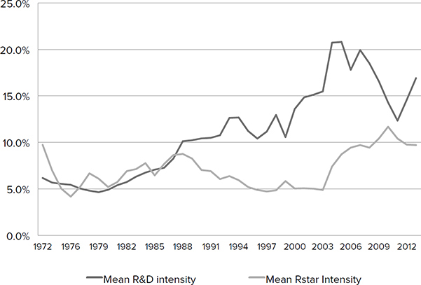
A pertinent example of rules of thumb gone wrong because of long lags between R&D and revenues comes from the pharmaceutical industry. For most of the 1970s, pharmaceutical companies invested roughly 5.5 percent of revenues in R&D, which was near optimal for them (Figure 4-3). Thus they were another example of reliable intuition despite the unavailability of RQ.

After that however, the pharmaceutical world was rocked by four major shifts. The first shift was the Health Maintenance Organization Act of 1973. This led to consolidation of buying power and ultimately the creation of formularies that restricted the set of reimbursable drugs. This enhanced power to restrict reimbursable drugs translated into lower drug prices and/or smaller markets. The second shift was a technological shift in drug discovery from a chemistry foundation to a biological foundation that coincided with the 1982 introduction of Humulin, the first biotech drug to achieve FDA approval. This shift meant that the technical expertise companies had developed over decades would become obsolete. The third shift was the Hatch-Waxman Act of 1984 that paved the way for generic drugs to compete with proprietary drugs immediately after patent expiration. This meant that the commercial life span of drugs and therefore total profits from a given drug were substantially reduced. The fourth and final shift affected marketing. When the FTC lifted its moratorium on direct-to-consumer (DTC) advertising in 1985, marketing emphasis shifted from detailing to doctors to advertising to consumers. Thus, not only were companies’ key technological resources becoming obsolete, so too were their marketing resources.

In response to these changes, pharmaceutical manufacturers began increasing R&D to about 8 percent of revenues. This trend toward increasing R&D intensity continued through 2004, reaching a peak at over 20 percent of revenues, four times what it had been in the 1970s! Unfortunately, pharmaceutical companies’ RQs began declining in 1989, such that firms were overinvesting in R&D. The gap between the actual and optimal R&D over all those years became forgone shareholder returns.

The pharmaceutical industry is an extreme example. In other contexts the world changes more slowly. One slow change that seemed to affect most large public companies was the increasing amount of CEO compensation tied to stock price. This made R&D an easy target when companies faced quarterly earnings pressure. Since R&D is expensed rather than capitalized, cuts yield immediate increases in profit, while the detrimental impact of those cuts isn’t felt for a few years. In marginal trade-offs between investments in physical capital or advertising whose returns are more easily quantified, R&D loses out. Evidence of this comes from companies’ response to the recent recession. On average, companies with revenues greater than $100 million reduced their R&D intensity by 5.6 percent on average, whereas capital intensity fell only 4.8 percent and advertising intensity actually increased 3.4 percent.

How Accurate Are the Rules of Thumb?

The pharmaceutical example and the investor pressure example illustrates what can go wrong with rules of thumb, but four out of five companies still use them, so maybe they’re reasonably effective. To examine that, I computed for each company in fiscal year 2014 what its optimal R&D budget would be, then compared that amount to what the company spent. This is shown in Figure 4-4. Each dot in the figure represents a company. Drawing a vertical line from a company to the x-axis identifies that company’s optimal R&D investment (on a logarithmic scale). Drawing a horizontal line from a company to the y-axis identifies that company’s actual R&D investment (also on a logarithmic scale). Companies that are investing optimally fall on the diagonal line. There are almost no companies on that line! In fact, only 4.6 percent of companies are within 10 percent of that line in either direction. Furthermore, of companies that invest over $100 million in R&D, there were only 16 such companies, which appear on the following list. What’s interesting about this list is that these companies don’t seem to have much in common, with the possible exception that five of them (those in bold) are still run by their founders.

Abbott Laboratories

Alexion Pharmaceuticals

Amazon

CareFusion Corp

First Solar

FMC Corp

Goodyear Tire & Rubber

Halliburton

Johnson Controls

MSCI

Netflix

Rockwell Automation

Sandisk

Schlumberger

Teradata

Waters

How Costly Are the Rules of Thumb?

We now know companies should be establishing their R&D budgets by setting the marginal dollar of R&D equal to the marginal dollar of gross profits generated by the R&D. We also know that only about 4.6 percent of companies are very close to that level of investment. So rather than optimizing their R&D, companies appear to be using rules of thumb, and those rules of thumb are not very good proxies for optimizing. The next question is, how costly is it for companies to use industry rules of thumb when setting their R&D budget?

To examine that I looked at the impact on profits of increasing R&D 10 percent for the 33 percent of companies that were underinvesting in R&D, as well as the impact of cutting R&D to the optimum level for the 63 percent of companies that were overinvesting. For the companies that were underinvesting, a 10 percent increase in R&D would increase profits $36 million on average. (I capped increases at 10 percent because growing R&D beyond 10 percent in a single period typically strains the organization.) For the companies that were overinvesting, reducing R&D by the amount of overinvestment would increase profits $258 million on average (note this average is driven by outliers).

The nice thing about solving the overinvestment problem is that it shows up in profits right away, so it should have an immediate impact on the company’s stock price. For the companies that are underinvesting, the gains from increased R&D won’t be felt as profits for a few years. However, if the market correctly values the expected increase in profits, these companies should also see the gains in stock price immediately.

I first flagged the suboptimal R&D investment problem in a 2012 article in Harvard Business Review (HBR). There I looked only at the top 20 companies and found the combined market value those companies were leaving on the table was one trillion dollars! The claim that companies were investing this poorly was bold, and not surprisingly it received a lot of criticism by bloggers at Atlantic and Forbes as well as in comments on the HBR article itself. The main complaint was that companies couldn’t be that far off.

Were the critics right? Since the article is now a few years old, I was able to rely on the test of time to answer that question. I looked at the performance of those 20 companies two years later (long enough for companies to implement the recommendations and begin to see results). Three of the companies no longer existed under the same name, so I restricted attention to the remaining 17 companies. I interpreted the companies’ decisions in terms of the direction of their R&D investment levels, rather than exact amounts—did they increase or decrease R&D investment? Of the 17 companies, 9 followed my recommendation, while the remaining 8 companies deviated from my recommendation.

The important question however was not what companies did, but rather what happened as a consequence of that. The nine companies that followed my recommendation showed an average profit increase of 16.4 percent. In contrast the eight companies that deviated from my recommendation showed an average profit decrease of 14.1 percent. This is by no means a statistically significant test. It involved only a handful of companies, all of whom have many other factors affecting their profits. However it does suggest the underlying prescriptions have merit.

So we know that underinvestment leaves $36 million of profits on the table each year, which is substantial in its own right. However, there is an even deeper problem with underinvestment. Prolonged underinvestment leads to deterioration in R&D capability. Starving the company of R&D cuts meat as well as fat. We saw this happen with GE and HP, but they are the rule rather than the exception.

THE PEANUT BUTTER PROBLEM

We now know that 80 percent of companies use rules of thumb in setting their R&D budgets. We also know they appear to be leaving shareholder money on the table as a result of doing this. Finally, we know the correct approach is to use RQ to identify the optimal target from the CFO’s office, and then to continue the bottoms-up approach to rank order projects and fund the highest-ranking projects until the target amount is reached.

The rank ordering of projects in this approach should ensure that the most valuable projects are funded. However, in multidivisional companies, one thing that might happen is that this rank ordering might produce a portfolio of R&D projects confined to a single division. This would occur if all projects in that division had higher expected returns than those in other divisions.

Typically the company would reject such a portfolio, since it wants all divisions to grow. Accordingly, in multidivisional companies another layer of targeting takes place. In addition to a single top-level target for the company, the CFO will apply industry specific benchmarks for R&D intensity to each division. This is what one CTO referred to as the “peanut butter approach” to R&D budgets. The problem with the peanut butter approach is that divisions differ in their RQ.

Across the companies I’ve worked with, the range of RQs across divisions has been as high as 30 RQ points (from the bottom sixth to the top sixth of companies). Since these data are highly confidential, let’s create a fictional example of what might happen in such a company (Table 4-1).

TABLE 4-1.  Fictional example of R&D budget in multi-divisional firm

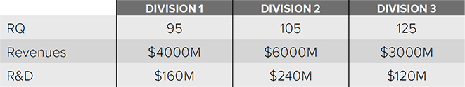
There are three divisions in our fictional company. Division 2, the largest division, has $6 billion in revenues and an above-average RQ of 105; Division 1 has $4 billion in revenues and a below- average RQ of 95; while Division 3, the smallest division, has revenues of $3 billion and a near-genius RQ of 125. Currently, the CFO allocates 4 percent of projected revenues to R&D for each division, so Division 1 gets $160 million, Division 2 gets $240 million, and Division 3 (which has the most productive R&D) gets the smallest amount—$120 million.

Let’s compare two budgeting scenarios for the upcoming year, both of which assume top-level growth of 5 percent, so the R&D budget increases 5 percent ($26 million). In the first scenario, the CFO once again follows the peanut butter approach, so Division 1 gets an additional $8 million in its R&D budget, Division 2 gets an additional $12 million, and Division 3 gets an additional $6 million (the light columns in Figure 4-5a).

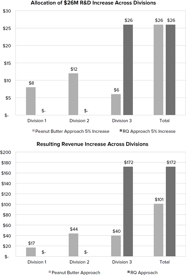
In the second scenario, the CFO allocates the additional R&D based on the marginal returns to R&D in each division, so Division 3 gets the entire $26 million in new R&D (the dark columns in Figure 4-5a).

The big question of course is what impact each of the two approaches has on revenues and profits. Looking first at the peanut butter approach, the additional $8 million in R&D to Division 1 yields $17 million in new revenues, the $12 million to Division 2 yields $44 million in new revenues, and the $6 million to Division 3 yields $40 million in new revenues. The total is an impressive $101 million in new revenues. If we assume gross profit margin is 50 percent, then the net profit from the new R&D is $24.5 million ($50.5 million in new gross margin; minus $26 million in new R&D).

Next let’s examine the RQ approach of allocating the R&D based on the marginal returns. Because there is no new R&D to Division 1 or Division 2, they have no new revenues from R&D. However Division 3, which obtains all the new R&D because of its high RQ, yields new revenues of $172 million. This is 70 percent higher than the revenues from the peanut butter approach! Making the same assumption about margins, the RQ approach yields $60 million in new profits ($86 million in new gross margin; minus $26 million in new R&D). This is two and a half times greater profits than the peanut butter approach!

Thus, one tremendous and immediate benefit of using the RQ approach of allocating R&D to divisions is that it yields substantially higher profits than the peanut butter approach. However, there is also a more important long-term, yet subtle benefit. Once the divisions know they are competing with one another for R&D based on their RQ, they will try to understand the factors contributing to Division 3’s higher RQ. Those efforts should lead to increases in RQ in the other divisions, which will lead to even higher profits.

WORKING THROUGH OPTIMAL INVESTMENT WITH TWO EXAMPLES

Let’s see what optimal investment looks like in two types of companies—an example from the 63 percent of companies that overinvest, AMD, and another example from the 33 percent of companies that underinvest, McKesson. Both companies are interesting examples because they are in the RQ50, the 50 companies with the highest RQs among the set of public companies investing at least $100 million in R&D each year. (We briefly review all the RQ50 firms in the Appendix.) Thus these are R&D exemplars in one sense, and yet even they have trouble identifying the appropriate levels of R&D.

We learned about Advanced Micro Devices (AMD) in the last chapter when we discussed its role in pressuring Intel to innovate. In fiscal year 2015, AMD reported $1.1 billion R&D investment. That’s substantially more than it should be investing. Given AMD’s RQ, a 10 percent increase in R&D should increase revenues to $115 million. This sounds great, but the problem, given AMD’s financials, is that the additional R&D ($107 million) exceeds the expected additional profits from that investment ($34 million). So AMD should shed projects that are ranked just below the $1.1 billion CFO target. If AMD does that, the company’s profits should increase by the amount R&D is reduced.

AMD is a single example, but 63 percent of companies are in the overinvestment boat with it. While getting these companies to spend optimally actually reduces R&D, it generates $215 billion in higher profits that could be redeployed more effectively.

AMD offers insight for the companies that overinvest in R&D. Now let’s look at the opposite problem, which is also prevalent—underinvestment in R&D. Here we’ll use McKesson as an example. McKesson is an outstanding company in many regards, only one of which is being in the RQ50. It is one of the oldest companies in the United States (founded in 1833). Very few companies live that long, and when they do they tend to become lumbering. Instead, McKesson is ranked 11 in the Fortune 500 and is the largest pharmaceutical and medical supplies distributor in North America.

However, for all its virtues, McKesson, like AMD, is investing suboptimally in R&D. The company reported $392 million R&D investment in 2015. This is a decrease of $64 million from 2014, but it should have been moving in the opposite direction. Given its RQ, increasing R&D 10 percent ($39.2 million) should increase revenues $7.5 billion! Even with its relatively slim operating margins (6.1 percent), that still yields $417 million in incremental profits. At the current P/E of 15.7, shareholders would increase their wealth $6.5 billion if McKesson increased its R&D 10 percent. We don’t recommend investing beyond that for two reasons: First, if R&D increases too dramatically, RQ will decrease. In addition, dramatically increasing resources typically leads to adjustment costs as the company tries to bring those resources online and integrate them with existing activities.

Again, McKesson is just one example, but 33 percent of companies are in the underinvestment boat with it. If all publicly traded underinvestors increased their R&D 10 percent, that would yield $16 billion in new profits.

RETURNING TO HP

In Chapter 1, I used the example of HP to demonstrate two problems that arise when companies lack reliable measures of R&D capability: (1) knowing whether HP’s capability had deteriorated and, if so, by how much, and (2) knowing whether 2 percent or 9 percent of sales was closer to the correct level of R&D investment. I addressed the first problem in Chapter 1. I showed that HP’s RQ had deteriorated substantially once neither founder was CEO. However, HP’s RQ began to increase under Mark Hurd.

Now I address the second issue of the correct level of R&D investment. It turns out that because HP’s RQ was declining, its optimal R&D intensity was also declining. Optimal R&D intensity increases with RQ because higher RQ companies get more bang from their R&D buck. Accordingly, it is optimal for them to spend more. In the case of HP, optimal R&D intensity fell from a high of between 5 and 6 percent under Dave Packard to a low of 2 percent when Mark Hurd became CEO. Thus Dave Packard was actually overinvesting in R&D, while Mark Hurd was investing optimally. So it is not the case that Mark Hurd was killing the innovation engine by cutting R&D. Rather, he was appropriately cutting the R&D investment because the engine had already deteriorated.

SUMMARY

Now we understand why tax credits won’t solve the problem of increasing innovation and growth. They are the government’s peanut butter approach to stimulating R&D. First, while the tax credits are very effective at increasing R&D, R&D in and of itself doesn’t increase growth. This is in part because RQ has been declining, but also because 63 percent of companies are already overinvesting in R&D. Increasing their R&D even more will further decrease profits. On the flip side, the 33 percent of companies that are underinvesting shouldn’t need tax credits to increase R&D. Increasing R&D will increase their profits even without tax credits.

We’ve shown that a better way to increase innovation and growth than the peanut butter approach of tax credits is using RQ to identify optimal levels of R&D, then increasing R&D in the companies and divisions that are underinvesting and decreasing R&D in the companies and divisions that are overinvesting.

What’s exciting about this approach is that everyone is better off. Shareholders in companies that are overinvesting increase the value of their stock by having those companies cut overinvestment. Shareholders in companies that are underinvesting increase the value of their stock by having those companies increase their R&D 10 percent. Further, because both corrections increase profits, the government gains corporate income tax on the higher profits and capital gains tax on the additional shareholder wealth. So the government increases revenues and saves the tax credits.