
A Note on Integral Equations
An integral equation contains an unknown function u under the integral sign. Integral equations represent one of the most powerful mathematical tools in mathematical physics and engineering. Integral equations appear in a variety of applications, usually being obtained from a corresponding differential equation as integral formulation often makes solution of the problem easier.
Linear integral equations are often analyzed and can be classified as Fredholm or Volterra equations. The Fredholm equations of the first and second kind can be written in the form:
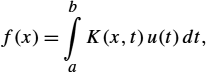
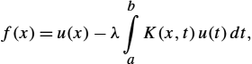
where λ is a parameter, ![]() is a function to be determined,
is a function to be determined, ![]() is the right-hand side and pertains to the excitation, and
is the right-hand side and pertains to the excitation, and ![]() is the integral equation kernel.
is the integral equation kernel.
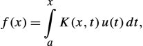
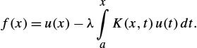
Furthermore, the Volterra equations of the first and second kind, having a variable upper limit of integration, are formulated as follows:
Note that integral equations (B.1) to (B.4) become homogeneous for ![]() . An integral equation is singular when either integration limits or kernel
. An integral equation is singular when either integration limits or kernel ![]() have infinite value. Furthermore, the kernel
have infinite value. Furthermore, the kernel ![]() is symmetric when a condition
is symmetric when a condition ![]() is satisfied.
is satisfied.
There is a close connection between the integral and differential formulation of a given problem. In general, differential equations can be expressed in terms of integral equations, but not vice versa. Whereas boundary conditions are imposed externally in differential equations, they are incorporated within an integral equation.
Thus, if one considers a first order differential equation and related boundary condition (Cauchy problem):
having performed the integration, Eq. (B.5) can be written as the Volterra integral of the second kind,
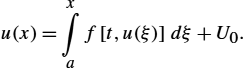
Since Eqs. (B.5) and (B.7) are equivalent, any solution of Eq. (B.7) satisfies both Eq. (B.5) and the prescribed boundary condition (B.6). Therefore, an integral equation formulation includes both the differential equation and the boundary condition(s).
Thus, the corresponding integral formulation contains a complete description of the given problem without necessity of defining additional boundary conditions.
Similarly, when integrating a second order ordinary differential equation (accompanied with corresponding boundary conditions),
the following formulation is obtained:

Integrating Eq. (B.9) by parts provides

Thus, (B.10) finally becomes

Obviously, the integral equation (B.11) represents both the differential equation (B.8) and the boundary conditions. Only one-dimensional integral equations have been discussed, but the approach could be extended to integral equations containing unknowns in two or more dimensions.
It is also worth noting that a majority of integral equations can be solved only by numerical methods.