
Theoretical Background: an Outline of Computational Electromagnetics (CEM)
Abstract
This chapter deals with fundamental concepts in electromagnetic theory and outlines some basics of numerical modeling. Thus, the chapter starts with Maxwell equations, continuity equation and Poynting theorem. Then, electromagnetic wave equations and potentials are derived, and finally, fundamentals of radiation are presented. The first part of the chapter ends with both analytical analysis of dipole antenna and Pocklington integro-differential equation approach. The second part of the chapter yields some introductory aspects of numerical methods. A brief description of finite element method (FEM), boundary element method (BEM) and numerical solution of integral equations over sources is given. Some simple computational examples are given, as well.
Keywords
Maxwell equations; continuity equation; radiation; antennas; finite elements; boundary elements; integral equation modeling
2.1 Fundamentals of Computational Electromagnetics
Rapid progress in the development of digital computers in mid-1960s enabled significant advancement in computational models.
Electromagnetic modeling provides the simulation of an electrical system electromagnetic behavior for a rather wide variety of parameters, for different initial and boundary conditions, excitation types, and different configuration of the system itself. Numerical modeling can be performed within a appreciably shorter time than it would be necessary for building and testing an appropriate prototype via experimental procedures. A basic purpose of a computational model in electromagnetics is to predict an object response to the external excitation generated by a certain EMI source. First, this section outlines some fundamental concepts in electromagnetic theory, then a short introduction to basic numerical methods is presented.
2.1.1 An Outline of Classical Electromagnetic Field Theory
Contributions of Faraday, Maxwell, Heaviside, Hertz and others resulted in the revolutionary concept of a field in classical physics, which was shown to be physically real, not just an abstract mathematical entity. As a consequence, through the notion of a field the actio in distans concept was abandoned [1].
In addition to establishing a rigorous electromagnetic field theory, James Clerk Maxwell managed to achieve a grand unification of electricity, magnetism and light. Namely, almost a quarter century before the Hertz experimental verification, Maxwell theoretically anticipated the existence of electromagnetic waves. Light is just an electromagnetic wave, visible to human eye propagating through ether. After Maxwell, H.A. Lorentz extended Maxwell's theory with electrodynamics of a charged particle.
Maxwell's equations were modified a few times [2] in the last 150 years, since they were originally formulated by Maxwell and published for the first time in [3]. The changes pertain to the physical interpretation, mathematical expression and an approach to the solution methods for different problems. In the mid-1860s, Maxwell originally derived 20 scalar equations, while a set of 4 vector equations was independently derived by Heaviside and Hertz by the end of the 19th century.
Important advancements of Maxwell's theory in the mid-1880s were carried out by Poynting, FitzGerald and Heaviside. Lorentz contribution is related to the development of a microscopic theory by means of Maxwell's equations and inclusion of the force acting on a charged particle arising from the existence of fields.
2.1.2 Maxwell's Equations – Differential and Integral Form
The laws of classical electromagnetism can be expressed in terms of four partial differential equations. There is also an equivalent integral form of these equations.
Originally, the governing equations of electromagnetics were derived in the time domain, but in many practical circumstances, particularly at low frequencies, systems are excited sinusoidally and a time-harmonic variation of electromagnetic fields can be assumed. In such cases it is convenient to represent the variables of interest in a complex phasor form. Thus, an arbitrary time dependent vector field F(r,t)![]() can be expressed as follows [4]:
can be expressed as follows [4]:
→F(→r,t)=Re[→Fs(→r)ejωt]
where Fs(r)![]() is the phasor form of F(r,t)
is the phasor form of F(r,t)![]() , and Fs(r)
, and Fs(r)![]() is in general complex with an amplitude and a phase changing with position. Then Re[] implies taking the real part of the quantity in brackets, and ω is the angular frequency of the sinusoidal excitation.
is in general complex with an amplitude and a phase changing with position. Then Re[] implies taking the real part of the quantity in brackets, and ω is the angular frequency of the sinusoidal excitation.
In addition, using the phasor representation, computing the derivatives with respect to time results in
∂∂t[→Fs(→r)ejωt]=jω→Fs(→r)ejωt.
The first Maxwell equation is the differential form of Faraday law (the time-changing magnetic flux density →B![]() causes the curl of electric field →E
causes the curl of electric field →E![]() ) given by
) given by
∇×→E=−∂→B∂t.
Hence, the time varying magnetic fields are vortex sources of electric fields.
The second Maxwell equation is the differential form of generalized Ampere's law stating that either a current density →J![]() or a time varying electric flux density →D
or a time varying electric flux density →D![]() gives rise to a magnetic field →H
gives rise to a magnetic field →H![]() :
:
∇×→H=→J+∂→D∂t.
It is worth noting that the term ∂→D/∂t![]() (displacement current density) was originally added by Maxwell to the original expression for Ampere's law, thus making the law consistent with the electric charge conservation.
(displacement current density) was originally added by Maxwell to the original expression for Ampere's law, thus making the law consistent with the electric charge conservation.
The third Maxwell equation states that charge densities ρ are the monopole sources of the electric field
∇⋅→D=ρ,
while the fourth Maxwell equation states that magnetic poles always occur in pairs, and are due to electric currents; no free poles can exist. This is expressed by the divergence Maxwell equation:
∇⋅→B=0,
stating that the magnetic field is always solenoidal.
The integral form of the Faraday law states that any change of magnetic flux density →B![]() through any closed loop induces an electromotive force around the loop. Taking the surface integral of (2.3) and applying the Stokes theorem yields
through any closed loop induces an electromotive force around the loop. Taking the surface integral of (2.3) and applying the Stokes theorem yields
∮c→E⋅d→s=−∫S∂→B∂t⋅d→S,
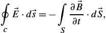
where the line integral is taken around the loop and with d→S=ˆndS![]() .
.
The voltage induced by a varying flux has a polarity such that the induced current in a closed path gives rise to a secondary magnetic flux which opposes the change in the time-varying source magnetic flux.
The integral form of Ampere's law is obtained by integrating (2.4) and applying the Stokes theorem:
∮c→H⋅d→s=∫S→J⋅d→S+∫S∂→D∂t⋅d→S.
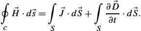
The generalized Ampere's law states that either an electric current or a time-varying electric flux gives rise to a magnetic field. Taking the volume integral of (2.5) and applying the Gauss divergence theorem yields
∮S→D⋅d→S=∫VρdV,
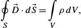
where right-hand side represents the total charge within the volume V.
Eq. (2.5) is the Gauss flux law for the electric field stating that the flux of →D![]() vector corresponds to the total electric charge within the domain.
vector corresponds to the total electric charge within the domain.
The Gauss flux law for the magnetic field can be derived by taking the volume integral of (2.6) and applying the Gauss divergence theorem, i.e.,
∮S→B⋅d→S=0,
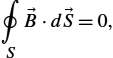
stating that the flux of →B![]() vector over any closed surface S is identically zero.
vector over any closed surface S is identically zero.
In linear, homogeneous and isotropic medium, one deals with the following constitutive equations:
→D=ε→E,
→J=σ→E,
→B=μ→H.
Furthermore, particle classical electromagnetics requires the Lorentz force equation
→F=q(→v×→B),
where q denotes the charged particle, →v![]() is the particle velocity, ε is permittivity, σ is conductivity, and μ is permeability of a medium, respectively.
is the particle velocity, ε is permittivity, σ is conductivity, and μ is permeability of a medium, respectively.
To solve Maxwell's equations for a given problem, the continuity conditions at the interface of two media with different electrical properties must be specified [5]:
ˆn×(→E1−→E2)=0,
ˆn×(→H1−→H2)=→Js,
ˆn⋅(→D1−→D2)=ρs,
ˆn⋅(→B1−→B2)=0,
where →n![]() is a unit normal vector directed from medium 1 to 2, subscripts 1 and 2 denote fields in regions 1 and 2. Eqs. (2.15) and (2.18) state that the tangential components of →E
is a unit normal vector directed from medium 1 to 2, subscripts 1 and 2 denote fields in regions 1 and 2. Eqs. (2.15) and (2.18) state that the tangential components of →E![]() and the normal components of →B
and the normal components of →B![]() are continuous across the boundary. Eq. (2.16) represents that the tangential component of →H
are continuous across the boundary. Eq. (2.16) represents that the tangential component of →H![]() is discontinuous by the surface current density →Js
is discontinuous by the surface current density →Js![]() on the boundary. Eq. (2.17) means that the discontinuity in the normal component of →D
on the boundary. Eq. (2.17) means that the discontinuity in the normal component of →D![]() is the same as the surface charge density ρs
is the same as the surface charge density ρs![]() on the boundary.
on the boundary.
In the case of perfect conductor, the electric field →E![]() and magnetic field →H
and magnetic field →H![]() vanish within the perfectly conducting medium. These fields are replaced by the surface charge density ρs
vanish within the perfectly conducting medium. These fields are replaced by the surface charge density ρs![]() and surface current density →Js
and surface current density →Js![]() . At higher frequencies there is a well-known effect which confines a current largely to surface regions.
. At higher frequencies there is a well-known effect which confines a current largely to surface regions.
As no time-varying field exists in a perfect conductor, the electric flux density is entirely normal to the conductor and supported by a surface charge density at the interface:
Dn=ρs.
The magnetic field is entirely tangential to the perfect conductor and is equilibrated by a surface current density:
Hs=Js.
Conditions at the extremes of the boundary value problem are obtained by extending the interface conditions.
Assuming the time-harmonic variation of fields, curl Maxwell's equations become:
∇×→E=−jω→B,
∇×→H=→J+jω→D.
It should be observed that the assumption of the time-harmonic variation of fields eliminates the time dependence from Maxwell's equations, thereby reducing the space-time dependence to space dependence only.
2.1.3 The Continuity Equation
The equation of continuity couples the electromagnetic field sources (the charges and current densities) and can be readily derived from Maxwell equation (2.4). Taking the divergence of the Maxwell equation (2.4) yields
∇⋅(∇×→H)=∇⋅→J+∇⋅(∂→D∂t).
As the left-hand side of (2.23) vanishes identically, it follows that
∇⋅→J+∂∂t(∇⋅→D)=0.
Invoking Gauss law (2.5), the equation of continuity is obtained, namely
∇⋅→J=−∂ρ∂t,
which for time-harmonic dependencies simplifies into
∇⋅→J=−jωρ.
The rate of charge moving out of a region is equal to the time rate of charge density decrease. The integral form of the continuity equation is obtained by performing the volume integration
∫V∇⋅→JdV=−∂∂t∫VρdV

and applying the Gauss divergence theorem
∫V∇⋅→JdV=∮S→J⋅d→S.

The integral form of the continuity equation is then given by
∮S→J⋅d→S=−∂Q∂t,
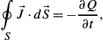
where the unit normal in d→S![]() is the outward-directed normal, and Q is the total charge within the volume
is the outward-directed normal, and Q is the total charge within the volume
Q=∫VρdV.

Eq. (2.29) represents the Kirchhoff conservation law widely used in the circuit theory.
2.1.4 Conservation of Electromagnetic Energy – Poynting Theorem
The general conservation law of energy in the macroscopic electromagnetic field can be readily derived from curl Maxwell equations. Starting from divergence of Poynting vector
∇⋅(→E×→H)=→H⋅∇×→E−→E⋅∇×→H
and combining (2.31) with Maxwell equations yields [1,6]
∇⋅(→E×→H)=−∂∂t(→E⋅→D+→H⋅→B2)−→E⋅→J.

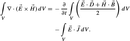
Taking the volume integral of (2.32) gives
∫V∇⋅(→E×→H)dV=−∂∂t∫V(→E⋅→D+→H⋅→B2)dV−∫V→E⋅→JdV.
For a battery with a non-electrostatic field →E′![]() pumping energy both into heat losses and into a magnetic field, the corresponding current density can be written as
pumping energy both into heat losses and into a magnetic field, the corresponding current density can be written as
→J=σ(→E+→E′).
Furthermore, applying the Gauss integral theorem to the left-hand side term, the volume integral transforms to the surface integral over the boundary, where d→S![]() is the outward drawn normal vector surface element, i.e., one obtains
is the outward drawn normal vector surface element, i.e., one obtains
∫V→E′⋅→JdV=∂∂t∫V12(→E⋅→D+→H⋅→B)dV+∫V|→J|σ⋅→JdV′+∮S(→E×→H)⋅d→S.
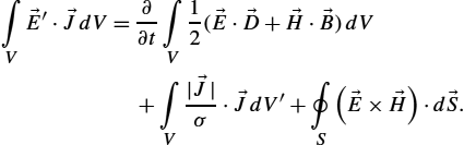
The sources within the volume of interest are balanced with the rate of increase of electromagnetic energy in the domain, the rate of flow of energy in through the domain surface and the Joule heat production in the domain.
The time-harmonic complex Poynting vector is given by
→S=12(→E×→H⁎).
Taking the divergence of Poynting vector yields
∇⋅→S=12(→H⁎⋅∇×→E−→E⋅∇×→H⁎).
The divergence of complex power density can be expressed in terms of a rate of stored energy, power losses and sources
∇⋅→S=−jω2(μ|→H|2−ε|→E|2)−|→J|σ+12σ|→E′|2.
Now the integration over a volume of interest yields
∫V∇⋅→SdV=−jω2∫V(μ|→H|2−ε|→E|2)dV=−12∫V|→Jσ|2dV+12∫Vσ|→E′|2dV.
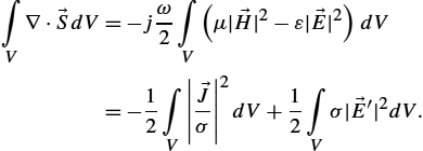
And applying the Gauss theorem, one obtains
12∫V→E×→H⁎⋅d→S=−jω2∫V(μ|→H|2−ε|→E|2)dV=−12∫V|→Jσ|2dV+12∫Vσ|→E′|2dV.

Finally, the real and imaginary parts, respectively, of the Poynting flow can be written as
12Re∫V→E×→H⁎⋅d→S=−12∫V|→Jσ|2dV+12∫Vσ|→E′|2dV,
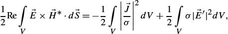
12Im∫V→E×→H⁎⋅d→S=−ω2∫V(μ|→H|2−ε|→E|2)dV.
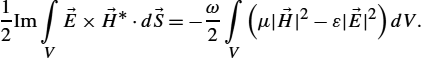
The real part of the integral over Poynting vector represents the total average power while the imaginary part of the integral over Poynting vector is proportional to the difference between average stored magnetic energy in the volume and average stored energy in the electric field.
The 12![]() factor appears because →E
factor appears because →E![]() and →H
and →H![]() fields represent peak values, and it should be omitted for root-mean-square (rms) values. The total average power can, for example, represent the radiated power by an antenna. In addition, the first volume integral on the right-hand side of (2.41) represents a power loss in the conduction currents and is just twice the average power loss.
fields represent peak values, and it should be omitted for root-mean-square (rms) values. The total average power can, for example, represent the radiated power by an antenna. In addition, the first volume integral on the right-hand side of (2.41) represents a power loss in the conduction currents and is just twice the average power loss.
2.1.5 Electromagnetic Wave Equations
The wave equations are readily derived from the Maxwell curl equations, by differentiation and substitution. Taking curl on both sides of (2.4) yields
∇×∇×→H=∇×→J+∂∂t(∇×→D).
Using constitutive equations (2.11) and (2.12) and assuming uniform scalar material properties yields
∇×∇×→H=σ∇×→E+ε∂∂t(∇×→E).
According to the Maxwell equation (2.3), curl of →E![]() is replaced by the rate of change of magnetic flux density:
is replaced by the rate of change of magnetic flux density:
∇×∇×→H=−μσ∂→H∂t−με∂2→H∂t2.

Performing some mathematical manipulations, similar equations can be derived for the electric field. Using the standard vector identity, valid for any vector →E![]() , namely
, namely
∇×∇×→H=∇⋅(∇⋅→H)−∇2→H,
and taking into account solenoidal nature of the magnetic field (2.6), the wave equation is obtained as
∇2→H−μσ∂→H∂t−με∂2→H∂t2=0.

If a linear, isotropic, homogeneous, source-free medium is considered, then the set of equations (2.47) simplifies into
∇2→H−1v2∂2→H∂t2=0,
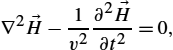
where v denotes the wave propagation velocity in lossless homogeneous medium,
v=1√με.
The velocity of wave propagation in free space is the velocity of light,
c=1√μ0ε0,
where c=3×10⁸![]() m/s, approximately.
m/s, approximately.
The complex phasor representation of the wave equation (2.47) results in the following equation of the Helmholtz type:
∇2→H−γ2→H=0,
where γ is the complex propagation constant given by
γ=√jωμσ−ω2με.
For a linear, isotropic, homogeneous, source-free medium, the Helmholtz equation (2.51) simplifies into
∇2→H+k2→H=0,
where k is a wave number of a lossless medium,
k=ω√με.
The complex form of potential wave equations could be derived similarly.
2.1.6 Electromagnetic Potentials
Instead of using fields, the analysis of classical electromagnetic phenomena can be simplified by using auxiliary potential functions, such as the electric scalar potential φ, or the magnetic vector potential →A![]() , which are readily derived from the Maxwell equations.
, which are readily derived from the Maxwell equations.
Thus, the divergence Maxwell equation (2.6) is satisfied if the flux density →B![]() is expressed in terms of an auxiliary vector function →A
is expressed in terms of an auxiliary vector function →A![]() , i.e.,
, i.e.,
→B=∇×→A.
Maxwell curl equation (2.5) then becomes
∇×→E=−∂∂t(∇×→A),
and, by rearranging (2.56), it follows that
∇×(→E+∂→A∂t)=0.
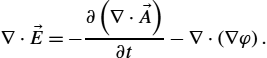
Now, the bracket quantity in (2.57) can be written as the gradient of the scalar potential function φ:
→E+∂→A∂t=−∇φ,
or
→E=−∂→A∂t−∇φ.
By using further mathematical manipulations, potential wave functions can be obtained. Thus, taking the divergence of (2.59), one obtains
∇⋅→E=−∂(∇⋅→A)∂t−∇⋅(∇φ).
Utilizing Gauss law yields
∇2φ+∂(∇⋅→A)∂t=−ρε.

Furthermore, from the second curl Maxwell equation (2.4) with (2.55), it follows that
∇×∇×→A=μ→J+με[−∇(∂φ∂t)−∂→A∂t]=0.

Now, using the vector identity
∇×∇×→A=∇(∇⋅→A)−∇2→A,
expression (2.62) can be written as
∇(∇⋅→A)−∇2→A=μ→J−με∇(∂φ∂t)−με∂2→A∂t2.

Now choosing the divergence of →A![]() as
as
∇⋅→A+με∂φ∂t=0,
expressions (2.61) and (2.64) become
∇2φ−με∂2φ∂t2=−ρε,
∇2→A−με∂2→A∂t2=−μ→J.
The set of Eqs. (2.66)–(2.67) can be regarded as a set of inhomogeneous potential wave equations for lossless media.
Thus, knowing the potential functions →A![]() and φ, the magnetic and electric fields can be determined from Eqs. (2.55) and (2.59).
and φ, the magnetic and electric fields can be determined from Eqs. (2.55) and (2.59).
The potential wave equations can be solved completely in a relatively small number of special cases. Integral solutions to potential wave equations (2.66) and (2.67) are given in the form of so-called retarded potentials [5,6]:
φ(→r,t)=14πε∫V′ρ(→r′,t−R/c)RdV′,

→A(r,t)=μ4π∫V′→J(→r′,t−R/c)RdV′,
where R is a distance from the source point to the observation point.
The solution of Eq. (2.69) is carried out by separating this vector equation into its Cartesian components. The result is a set of equations identical in form to the scalar potential equation. Recombining these components results in the solution (2.69).
If all electromagnetic quantities of interest are varying harmonically in time, the particular integrals for the retarded potentials are given by [5,6]:
φ(→r)=14πε∫V′ρ(→r′)e−jkRRdV′,
→A(r)=μ4π∫V′→J(→r′)e−jkRRdV′,

while the complex notation ejωt![]() is understood and omitted.
is understood and omitted.
2.1.7 Plane Wave Propagation
Plane waves are a satisfactory approximation for many realistic scenarios, e.g., radio waves at large distances from the transmitter, or from scattering obstacles having negligible curvature, and are well represented. Moreover, complicated wave patterns can be considered as a superposition of plane waves. Finally, the basic ideas of propagation, reflection and refraction in the plane wave approach are useful in understanding of more complex wave problems.
Considering the case of source-free homogeneous medium and the x-component of the vector field intensity and assuming there is no variation of the fields in both x and y directions, the corresponding Helmholtz equation for the electric field is given by
∂2Ey∂x2=−k2Ey.
The related solution can be written as
Ey=Ae−jkx+Be+jkx,
where k is the wavenumber of the corresponding lossless medium defined by relation (2.54), A and B are the magnitudes of forward and backward wave, respectively.
There is no variation of the field quantities in the plane perpendicular to the propagation direction, therefore the wave is simply called a plane wave. As a medium is unbounded, only the forward wave exists:
Ey=E0e−jkx,
where E0![]() denotes the magnitude of the electric field.
denotes the magnitude of the electric field.
The corresponding plane wave is shown in Fig. 2.1.

The corresponding magnetic field can be obtained from the time-harmonic curl Maxwell equation
∇×→E=−jωμ→H.
Furthermore, it follows that
→H=−1jωμ|ˆexˆeyˆez∂∂x000Ey0|=−ˆez1jωμ∂Ey∂x,

and the corresponding magnetic field is
Hz=E0Z0e−jkx=H0e−jkx,
where
Z0=E0H0=√με
is the wave impedance of the medium. For free space it is approximately Z0=120π![]() .
.
Now the space-time notation can be used:
Ey(x,t)=Re[E0ej(ωt−kx)],
and the electric and magnetic fields can be written as follows:
Ey(x,t)=E0cos(ωt−kx),
Hz(x,t)=E0Z0cos(ωt−kx).
Note that in circuit theory, contrary to electromagnetism, a sinusoidal dependence, rather than cosinusoidal, is chosen.
2.1.8 Radiation and Hertz Dipole
Electromagnetic radiation is a phenomenon caused due to the acceleration of charged particles. Fields generated by accelerated charges can be analyzed by using microscopic approach, dealing with individual particles, or by using the macroscopic approach within which average fields over the charge distributions are considered [7,8].
The choice of the particular approach depends on whether the observation times and distances are smaller or higher than the characteristic times and distances associated with the sources [7,8].
A macroscopic viewpoint of radiation is provided by Maxwell equations from which the radiated fields due to their sources in terms of charge and current densities are presented. In particular, radiation from thin wires can be rigorously analyzed by a corresponding type of either space-frequency or space-time integral equation, respectively.
Thus, radiation of electromagnetic energy is an undesired leakage phenomenon or a desired process for exciting waves in space. In the case of desired radiation, the goal is to excite waves from the given source in the required direction, as efficiently as possible. The matching unit between the source and waves in space is known as the radiator, antenna or areal. The results developed for radiating or transmitting antennas can be applied to the same antenna when used for receiving applications if antenna does not contain active components (the principle of reciprocity). The relation of the radiating case to the receiving situation can be made rigorously by means of the so-called principle of reciprocity [9].
The simplest radiating system is that of an ideal short linear element (Hertz dipole) with current considered uniform over its entire length. More complex antenna structures can be considered to be composed from infinite number of such elementary antennas with the corresponding magnitudes and phases of their currents.
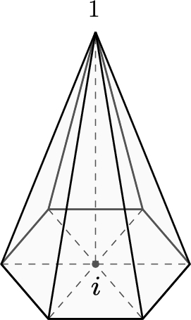
The current element, usually called Hertzian dipole, oriented in the z-direction, with its location at the origin of a set of spherical coordinates, is shown on Fig. 2.2.
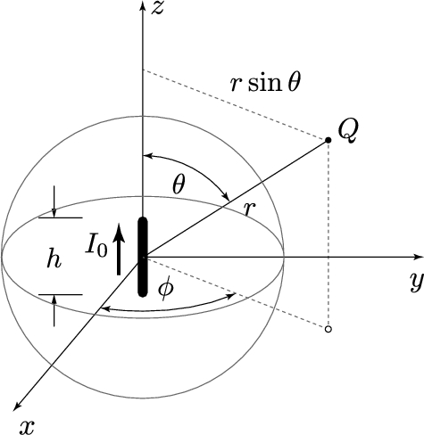
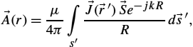
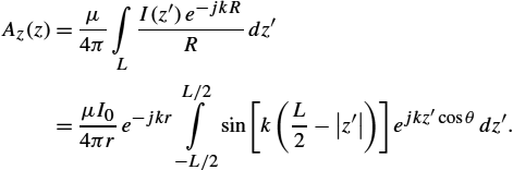
The length h of this electrically short antenna is very small compared to wavelength. As the wire radius a is small compared to the wavelength, the particular integral for retarded potential can be written in the form
→A(r)=μ4π∫s′→J(→r′)→Se−jkRRd→s′,
which results in
→A(z)=μ4π∫LI(z′)e−jkRRˆedz′,

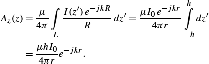
and finally, if the current along the short antenna is assumed to be constant and expressed in the following phasor form:
I(z′)=I0,
one obtains the final expression for the related retarded potential:
Az(z)=μ4π∫LI(z′)e−jkRRdz′=μI0e−jkr4πrh∫−hdz′=μhI04πre−jkr.
If the system of spherical coordinates is considered, then
Ar=Azcosθ=μhI04πre−jkrcosθ,
Aθ=−Azsinθ=−μhI04πre−jkrsinθ.
Combining the complex phasor form of Eqs. (2.59) and (2.65) gives
→E=−jω→A−∇φ,
∇→A=−jωμεφ,
and then the electric field can be expressed as follows:
→E=−jω→A+1jωμε∇(∇⋅→A).
Finally, the field components become:
Hϕ=hI04πe−jkr(jkr+1r2)sinθ,
Er=hI04πe−jkr(2Z0r2+2jωεr3)cosθ,
Eθ=hI04πe−jkr(jωμr+1jωεr3+Z0r2)sinθ.
At large distances from the source (r≫λ![]() ), the only significant terms for E and H are those varying as 1/r
), the only significant terms for E and H are those varying as 1/r![]() . This is the region where the far field is significant and the corresponding components are:
. This is the region where the far field is significant and the corresponding components are:
Hϕ=jkhI04πre−jkrsinθ,
Eθ=jωμhI04πre−jkrsinθ=Z0Hϕ.
The total power collected in the far field can be obtained by using expression (2.41). Namely, the total power is the integral of the time average Poynting vector over any surrounding surface. For simplicity this surface is a sphere of radius r:
P=∮S12Re(→E×→H⁎)d→S=2π∫0π∫012Re(EθH⁎φ)r2sinθdθdφ=Z0k2I20h216ππ∫0sin3θdθ=Z0πI203(hλ)2.
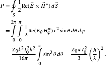
As the power radiated by the electrically short antenna is proportional to the squared value of the ratio h/λ![]() , the Hertzian dipole with the entire length h is rather small compared to wavelength λ and represents a radiator with a very small efficiency.
, the Hertzian dipole with the entire length h is rather small compared to wavelength λ and represents a radiator with a very small efficiency.
2.1.9 Fundamental Antenna Parameters
To describe antenna properties, it is necessary to define various parameters. Some of the parameter definitions specified in [5] are given in this chapter.
2.1.9.1 Radiation Power Density
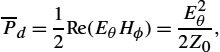
The power density of an antenna corresponds to the real part of the time average Poynting vector, and for the case of a free space it follows that
‾Pd=12Re(EθHϕ)=E2θ2Z0,
where Eθ![]() and Hϕ
and Hϕ![]() are the maximal (peak) values of the electric and magnetic fields, respectively. If the rms values are considered, then (2.97) becomes
are the maximal (peak) values of the electric and magnetic fields, respectively. If the rms values are considered, then (2.97) becomes
‾Pd=E2θZ0.

In the far field region, Eθ![]() and Hϕ
and Hϕ![]() vary as 1/r
vary as 1/r![]() and thus ‾Pd
and thus ‾Pd![]() varies as 1/r2
varies as 1/r2![]() .
.
2.1.9.2 Radiation Intensity
Radiation intensity, or the antenna power pattern, in a given direction is defined as the power radiated from an antenna per unit solid angle. The radiation intensity is a far field parameter which can be obtained by simply multiplying the radiation power density by the square distance, i.e.,
U=r212Re(EθHϕ)=r212EθZ0.
The relationship between the total power and radiation intensity is given by
Prad=∮ΩUdΩ=2π∫0π∫0Usinθdθdϕ,
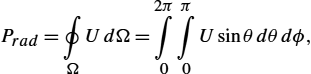
where dΩ=sinθdθdϕ![]() .
.
In particular, for an isotropic source, Eq. (2.100) becomes
Prad=∮ΩU0dΩ=4πU0,

or equivalently, the radiation intensity of an isotropic source is given by
U0=Prad4π.
As is obvious, the radiation intensity U is independent of the angles ϕ and θ.
2.1.9.3 Directivity
Directivity of an antenna is defined as the ratio of the radiation intensity in a given direction from the antenna to the radiation intensity averaged over all directions. The average radiation intensity is equal to the total power radiated by the antenna divided by 4π. If the direction is not strictly specified, the direction of maximum radiation intensity is implied.
Namely, the directivity D of a non-isotropic source is equal to the ratio of its radiation intensity in a given direction over that of an isotropic source:
D=UU0=4πUPrad.
If the direction is not specified, it implies the direction of maximum radiation intensity (maximum directivity) determined as
Dmax=UmaxU0=4πUmaxPrad,
where Dmax![]() is the maximum directivity, U0
is the maximum directivity, U0![]() is radiation intensity of isotropic source and Umax
is radiation intensity of isotropic source and Umax![]() is the maximum radiation intensity. To summarize, directivity is a measure that describes only the directional properties of the antenna, and it is therefore controlled only by the pattern.
is the maximum radiation intensity. To summarize, directivity is a measure that describes only the directional properties of the antenna, and it is therefore controlled only by the pattern.
2.1.9.4 Input Impedance, Radiation and Loss Resistance
Input impedance is defined as the ratio of the voltage and current at the pair of the input antenna terminals:
Za=Ra+jXa,
where Ra![]() is the resistance at antenna terminals and Xa
is the resistance at antenna terminals and Xa![]() is the reactance at antenna terminals.
is the reactance at antenna terminals.
In addition, the resistive part of (2.105) consists of two components:
Ra=Rr+RL,
where Rr![]() is the radiation resistance, and RL
is the radiation resistance, and RL![]() is the loss resistance of the antenna.
is the loss resistance of the antenna.
The radiation resistance Rr![]() is defined as the ratio of the total power radiated by the antenna P0
is defined as the ratio of the total power radiated by the antenna P0![]() and the square of the rms antenna input current I:
and the square of the rms antenna input current I:
Rr=P0I2.
If the peak value of the current is considered, then
Rr=P02I2m.
This is an equivalent resistance that would dissipate a power equal to the total radiated power when the current through it were equal to the antenna input current.
2.1.9.5 Gain and Radiation Efficiency
Antenna gain is closely related to the directivity, but it is also a measure that takes into account the efficiency of the antenna. The gain of an antenna in a given direction is defined as the ratio of the intensity, in a given direction, and the radiation intensity that would be obtained if the power accepted by the antenna were radiated isotropically. This is called the absolute gain. The radiation intensity corresponding to the isotropically radiated power is equal to the power input by the antenna divided by 4π. Thus,
G(ϕ,θ)=4πU(ϕ,θ)Pin,
where Pin![]() is the total input power.
is the total input power.
However, in most cases, one deals with a relative gain which is often defined as the ratio of the power gain in a given direction and the power gain of a reference in its referenced direction. The power input has to be the same for both antennas. The reference antenna is usually a dipole, horn, or any other antenna whose gain can be determined or is known.
In most cases, however, the reference antenna is a lossless isotropic source.
When the direction is not stated, the power gain is usually taken in the direction of maximum radiation.
In addition, the total radiated power Prad![]() is related to the total input power Pin
is related to the total input power Pin![]() , hence, it follows that
, hence, it follows that
Prad=ePin,
where e is the antenna radiation efficiency defined as the ratio of the power delivered to the radiation resistance Rr![]() and radiation losses RL
and radiation losses RL![]() :
:
e=RrRr+RL.
Radiation efficiency can be considered as a measure of the dissipative or heat losses in an antenna. It is worth noting that impedance mismatch losses at the input port of the antenna are not included in the radiation efficiency.
Taking into account (2.110), Eq. (2.111) becomes
G(ϕ,θ)=e[4πU(ϕ,θ)Prad],
which is related to the directivity by the expression
G(ϕ,θ)=eD(ϕ,θ).
In many applications, partial gains Gϕ![]() and Gθ
and Gθ![]() are used. These partial gains are defined as:
are used. These partial gains are defined as:
Gϕ=4πUϕPin,
Gθ=4πUθPin,
where Uϕ![]() is the radiation intensity in a given direction contained in the ϕ-field component, Uθ
is the radiation intensity in a given direction contained in the ϕ-field component, Uθ![]() is the radiation intensity in a given direction contained in the θ-field component, and Pin
is the radiation intensity in a given direction contained in the θ-field component, and Pin![]() is total input power.
is total input power.
Usually, the gain is given in terms of decibels instead of the dimensionless quantity.
2.1.10 Dipole Antennas
The finite length wire antennas (linear antennas) can be modeled as a superposition of infinitesimal radiation sources. Antenna problem can be considered in two different modes: radiation (transmitting) mode and scattering (receiving) mode.
The key to understanding the behavior of radiated or scattered fields is the knowledge of the current distribution induced along the antenna. For the case of electrically short wires where the length is small compared to the wavelength, the current can be approximated as a constant (as in the case of Hertz dipole) or linear function. On the other hand, if the wire length or frequency increases, the current distribution changes significantly. There are several approaches to determine the current distribution of a linear antenna. The simplest way is to assume the current waveform. Even though such an approach could provide satisfactory results in many applications, if thin wires are considered, there are situations where an accurate current distribution calculation is necessary. A more rigorous approach to this problem is to obtain the current distribution by solving the corresponding integral equation, which is discussed in details in Sect. 2.1.11. This section deals with the approximate current distributions.
One of the simplest antennas most commonly used in practice and also as an EMC model is the center-fed dipole antenna shown in Fig. 2.3. The entire length of the wire is L.
At high frequencies the reasonable and traditionally widely used approximation for the antenna current is the sinusoidal distribution defined as
I(z)=I0sin[k(L2−|z|)].
At sufficiently low frequencies where λ>L/2![]() , i.e., k(L/2−|z|)≪1
, i.e., k(L/2−|z|)≪1![]() , Eq. (2.116) becomes
, Eq. (2.116) becomes
I(z)=I0(1−2|z|L).
Approximating the distance from the source to the observation point gives
R=r−z′cosθ.
The radiated far field Eθ![]() , where the following condition is satisfied:
, where the following condition is satisfied:
kr=2πrλ≫1,
can be determined from the magnetic vector potential
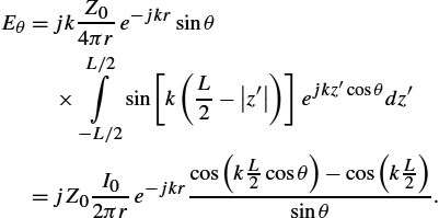
Eθ=−jωAθ=jωAzsinθ,
where the magnetic vector potential for the case of sinusoidal current distribution is given by
Az(z)=μ4π∫LI(z′)e−jkRRdz′=μI04πre−jkrL/2∫−L/2sin[k(L2−|z′|)]ejkz′cosθdz′.
Combining Eqs. (2.120) and (2.121) yields
Eθ=jkZ04πre−jkrsinθ×L/2∫−L/2sin[k(L2−|z′|)]ejkz′cosθdz′=jZ0I02πre−jkrcos(kL2cosθ)−cos(kL2)sinθ.
In the far-field region, the magnetic and electric field are related, and one obtains
Hϕ=EZ0=jI02πre−jkrcos(kL2cosθ)−cos(kL2)sinθ.

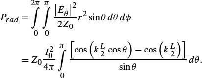
Finally, the total power radiated by the dipole antenna can be obtained from integral (2.41), i.e.,
Prad=2π∫0π∫0|Eθ|22Z0r2sinθdθdϕ=Z0I204ππ∫0[cos(kL2cosθ)−cos(kL2)]sinθdθ.
The radiation resistance is defined by relation (2.108). For the case of half-length dipole, the total power is
Prad=Z0I204ππ∫0cos2(kL2cosθ)sinθdθ.
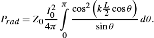
The radiation resistance of half-length dipole is approximately equal 73Ω.
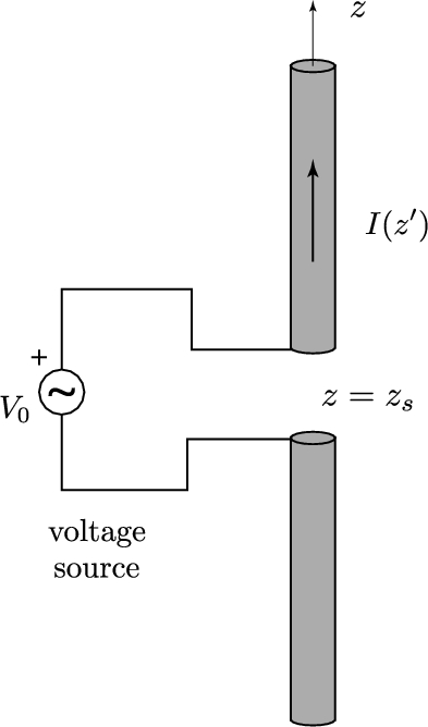
2.1.11 Pocklington Integro-Differential Equation for a Straight Thin Wire
Henry Cabourn Pocklington was the first who formulated the frequency domain integro-differential equation for a total current flowing along a straight thin wire antenna in 1897 [10]. He also presented the first approximate solution of this equation. During the last 120 years, many outstanding researchers have investigated both the formulation and the numerical solution of the Pocklington equation. Maybe the most important advance in the formulation was carried out by Erik Hallén in the late 1930s. Having started from Pocklington integro-differential equation in the frequency domain, Hallén managed to derive a new type of integral equation for thin wire configurations. Since than, many numerical techniques for solving the Pocklington and Hallén equation, respectively, were reported by different authors [6].
Numerical modeling of the wire antennas and scatterers started in 1965 with the classical paper by K.K. Mei [11]. Mei derived certain types of Pocklington and Hallén equation, having also reported a related numerical technique for solving these equations. Today his technique could be referred to as the point-matching technique. A number of important contributions to the numerical solution of Pocklington and Hallén integral equations were given in the 1970s: Silvester and Chan (1972, 1973) [12,13], proposed the use of the strong finite element formulation to the Hallén and Pocklington equations, while Butler and Wilton (1975, 1976) [14,15], proposed several moment method techniques for solving these equations.
In addition to the improvement in development of numerical solution methods, there have been important achievements in the formulation of the problem. Thus, the most important outcome is the extension of the original Pocklington formulation to the wires radiating in the presence of an imperfectly conducting half-space. This was worked out by E.K. Miller et al. (1972) [16], T. Sarkar (1977) [17] and by Parhami and Mittra [18]. The numerical solution of Pocklington equation via Galerkin–Bubnov Indirect Boundary Element Method (GB-IBEM) was reported elsewhere, e.g., in [6].
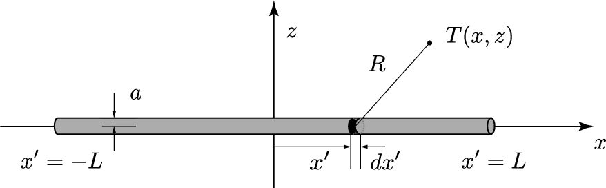
Consider a dipole antenna insulated in free-space having length L and radius a, as shown in Fig. 2.4.
The dipole antenna parameters of interest describing its radiating behavior can be determined, provided its axial current distribution is known. This current flowing along the thin wire antenna is governed by the frequency domain Pocklington integro-differential equation. The Pocklington equation can be derived in a few ways starting from Maxwell equation for time harmonic fields.
The thin wire approximation requires wire dimensions to satisfy the conditions:
a≪λ0anda≪L,
where λ0![]() is the wavelength of a plane wave in free-space.
is the wavelength of a plane wave in free-space.
Consequently, only axial component of →A![]() exists along the wire, and (2.92) can be written as
exists along the wire, and (2.92) can be written as
Ex=1jωμε0[∂2Ax∂x2+k2Ax].

The magnetic vector potential Ax![]() is expressed by a particular integral over the unknown axial current I(x)
is expressed by a particular integral over the unknown axial current I(x)![]() along the wire:
along the wire:
Ax=μ4πL∫−LI(x′)e−jkRRdx′,
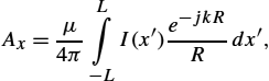
where R is a distance from the source point to the observation point and k is the wave number of free-space.
Assuming the wire to be perfectly conducting (PEC), and according to the continuity conditions for the tangential electric field components, the total tangential electric field vanishes on the PEC wire surface:
Eincx+Esctx=0,
where Eincx![]() is the incident field and Esctx
is the incident field and Esctx![]() is the scattered field due to the presence of the PEC surface. Inserting (2.128) into (2.127), the electric field scattered from the antenna surface becomes
is the scattered field due to the presence of the PEC surface. Inserting (2.128) into (2.127), the electric field scattered from the antenna surface becomes
Escax=1j4πωε0L∫−L(∂2∂x2+k2)g0(x,x′)I(x′)dx′.

Combining (2.129) and (2.130) leads to the Pocklington integro-differential equation for the unknown current distribution along the single straight wire antenna insulated in free-space:
Eincx=−1j4πωε0L∫−L(∂2∂x2+k2)g0(x,x′)I(x′)dx′,
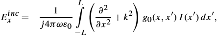
where g0(x,x′)![]() is the free-space Green function,
is the free-space Green function,
g0(x,x′)=e−jkRR,
while the distance R from the source to the observation point is
R=√(x−x′)2+a2.
Once the axial current on the antenna is determined, other important antenna parameters, such as radiated field, radiation pattern, or input impedance, can be calculated. The details can be found elsewhere, e.g., in [6].
Very similar derivation could be undertaken for imperfectly conducting wires. Studies for thin wires in the presence of inhomogeneous media could be found elsewhere, e.g., in [1] and [6]. Numerical solution of integro-differential equation (2.131) is discussed in Sect. 2.2.
2.2 Introduction to Numerical Methods in Electromagnetics
Problems arising in electromagnetics can be formulated in terms of differential, integral or variational equations. Generally, there are two basic approaches to solve problems in electromagnetics; the differential, or the field approach, and integral, or the source approach.
The field approach deals with a solution of a corresponding differential equation with associated boundary conditions, specified at a boundary of a computational domain. Such an approach is rather useful for handling the interior field problems; see Fig. 2.5.

A standard boundary-value problem can be formulated in terms of the operator equation
L(u)=p
on the domain Ω with conditions F(u)=q|Γ![]() prescribed on the boundary Γ (see Fig. 2.5), where L
prescribed on the boundary Γ (see Fig. 2.5), where L![]() is a linear differential operator, u solution of the problem, and p is the excitation function representing the known sources inside the domain. Methods for the solution of the interior field problem are generally referred to as differential methods, or field methods.
is a linear differential operator, u solution of the problem, and p is the excitation function representing the known sources inside the domain. Methods for the solution of the interior field problem are generally referred to as differential methods, or field methods.
The source, or the integral approach, is based on the solution of a corresponding integral equation. The source approach is convenient for the treatment of the exterior field problems, see Fig. 2.6.

The integral formulation can be generally written as follows:
g(u)=h,
where g represents an integral operator, unknowns u are related to field sources, i.e., charge densities or current densities distributed along the boundary Γ′![]() , while h is an excitation function (see Fig. 2.6), e.g., the electric field illuminating the metallic object, thus inducing the charge density. Once the sources are determined, the field at an arbitrary point, inside or outside the domain, can be obtained by integrating the sources.
, while h is an excitation function (see Fig. 2.6), e.g., the electric field illuminating the metallic object, thus inducing the charge density. Once the sources are determined, the field at an arbitrary point, inside or outside the domain, can be obtained by integrating the sources.
The methods of solutions for the exterior field problems are referred to as the integral methods, or methods of sources.
The boundary conditions used in electromagnetic field problems are usually of the Dirichlet (forced) and Neumann (natural) type, or their combination (mixed boundary conditions) [6,19]. These boundary conditions can be either homogeneous or inhomogeneous.
Operator equations can be handled analytically and/or numerically. Analytical solution methods yield exact solutions, but are limited to a narrow range of applications, mostly related to canonical problems. There are few practical engineering problems that can be solved in closed form. Numerical methods are applicable to almost all scientific engineering problems, with the main drawbacks pertaining to the approximation limit in the model itself, space and time discretization. Moreover, the criteria for accuracy, stability and convergence are not always straightforward and clear to the researcher. The most commonly used methods in computational electromagnetics (CEM), among others, are the Finite Difference Method (FDM), Finite Element Method (FEM), Boundary Element Method (BEM), and Method of Moments (MoM).
The problems being analyzed can be regarded as steady state or transient, and the solution methods are usually classified as frequency or time domain. The frequency and time domain techniques for solving transient electromagnetic phenomena have been fully documented in [6].
A frequency domain solution is commonly applied for many sources and a single frequency, whereas with the time domain, it is for a single source and many frequencies [6].
The time domain solution obtained is specific to the temporal variation of the excitation source. The transient response of a structure when subjected to different excitations, for example, a step-function or a Gaussian voltage source, will require the computation process to be repeated for the respective solutions, whereas in the frequency domain approach, the solution from one set of computations can be applied to obtain transient results from different sources if the geometry of the structure is unchanged. This difference is a significant factor when considering the relative merits of the two approaches.
Generally, a deeper physical insight is obtained when using the time domain approach. However, an understanding of the resonant characteristic can only be obtained from the frequency spectrum. Furthermore, nonlinearities are more conveniently handled in the time domain. Frequency domain formulation is definitely simpler and easier to use, thus allowing more complex structures to be analyzed more conveniently as for such geometries larger computing effort is required in the time domain approach.
According to the differential and integral formulation, numerical methods per se can be classified as domain, boundary or source simulation methods.
It is important to clarify some principles and ideas of how to describe field problems via partial differential or integral equations. Namely, there are some basic differences between domain methods (e.g., finite element method), boundary methods (e.g., boundary element method) and source simulation methods (charge or current simulation method). This section outlines some basics of Finite Element Method (FEM), as well as direct and indirect Boundary Element Method (BEM). Some basics regarding modeling via the Finite Difference Method (FDM) could be found elsewhere, e.g., in [6].
Finite element method (FEM) modeling of partial differential equations is undertaken by discretizing the entire calculation domain Ω, and integrating any known sources Ωs![]() (if any) within the domain, see Fig. 2.7A. Dirichlet and Neumann boundary conditions are specified along the boundary Γ for both FDM and FEM. Finally, an algebraic equation system provides a sparse matrix, usually banded and in many cases symmetric.
(if any) within the domain, see Fig. 2.7A. Dirichlet and Neumann boundary conditions are specified along the boundary Γ for both FDM and FEM. Finally, an algebraic equation system provides a sparse matrix, usually banded and in many cases symmetric.

Modeling via the Boundary Integral Equation Method involves direct and indirect approach. Integral formulations of partial differential equations along the boundary are carried out using the Green integral theorem. The resulting equations are modeled discretizing only the boundary and by integrating any known sources Ωs![]() within a given subdomain. Typically, modeling of partial differential equations in terms of related boundary integral formulations results in less unknowns but dense matrices [6].
within a given subdomain. Typically, modeling of partial differential equations in terms of related boundary integral formulations results in less unknowns but dense matrices [6].
The boundary element approach method using field and potential quantities rather than field sources is usually referred to as the direct BEM formulation. However, there are many applications in computational electromagnetics of boundary integral formulation for which it is more convenient to deal with sources. Such an approach is known as direct BEM, and related integral equations are posed in terms of sources distributed over the boundary. This method can be considered as a special case of the direct BEM approach involving integration over unknown charge density or current density. Integral equations over unknown sources Ω′s![]() (see Fig. 2.7B) can also be derived from the Green integral theorem, and the solution method can be referred to as a special variant of the boundary element method – indirect boundary element method.
(see Fig. 2.7B) can also be derived from the Green integral theorem, and the solution method can be referred to as a special variant of the boundary element method – indirect boundary element method.
However, as classic BEM uses potential or field on the domain boundary and this integral equation approach deals with unknown sources, some authors use the term finite elements for integral operators [19]. On the other hand, in order to stress the integration over sources, the term source element method (SEM) or source integration method (SIM) is suggested [6].
2.2.1 Weighted Residual Approach
Partial differential equations (PDEs), integral equations (IEs) and integro-differential equations (IDEs) are modeled using the weighted residual approach, also referred to as a projection approach [19].
Assume one seeks a solution of an operator differential equation
L(q,t)=0,
where L![]() is a corresponding differential operator.
is a corresponding differential operator.
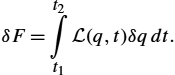
Now, within the variational formalism, differential (operator) equation can be regarded as a Lagrange equation, thus it can be written as
δF=t2∫t1L(q,t)δqdt.
On the other hand, in the framework of Galerkin procedure, construction of a corresponding functional is not required, therefore, it is of interest to write the variation of the functional in a way that the differential equation is multiplied by an arbitrary function and integrated.
Provided that the variation of the functional is zero, it can be written as
t2∫t1L(q,t)ψ(t)dt=0,

where the expression
t2∫t1L(q,t)ψ(t)dt

is regarded as a scalar product of functions L![]() and ψ.
and ψ.
It is worth noting that the requirement for the integral to vanish is equivalent to the orthogonality of these functions. The first step is to derive the formulation for an approximation of functions.
2.2.1.1 Fundamental Lemma of Variational Calculus
The fundamental lemma of variational calculus can be outlined as follows: scalar product of functions u and W in an n-dimensional Hilbert space is defined by the integral
〈u,W〉=∫Ωu(x)⋅W⁎(x)dΩ,x∈Ω,

where W⁎(x)![]() stands for the complex conjugate of W(x)
stands for the complex conjugate of W(x)![]() . If for a given function u and an arbitrary function W, the scalar product vanishes
. If for a given function u and an arbitrary function W, the scalar product vanishes
∫Ωu(x)⋅W⁎(x)dΩ=0,x∈Ω,

then it follows that
u(x)≡0,x∈Ω.
Defining u(x)![]() as a residual (difference between an exact function f and approximate function ˜f
as a residual (difference between an exact function f and approximate function ˜f![]() ),
),
u(x)=f−˜f,
according to the fundamental lemma of variational calculus, the residual integral vanishes
∫Ω(f−˜f)WdΩ=0

for an arbitrary function W only if f=˜f![]() .
.
An approximate function can be expressed in terms of a linear combination
˜f=n∑i=1αiNi(x).

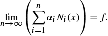
Note that the series converges only in the case
limn→∞(n∑i=1αiNi(x))=f.
The residual integral can be written in the following form:
∫Ω[f−n∑i=1αiNi(x)]WjdΩ=0,j=1,2,…,n,

where Wj![]() stands for a set of test (weighting) functions.
stands for a set of test (weighting) functions.
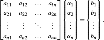
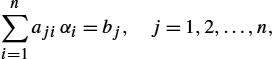
The weighted residual integral is transformed into a set of linear equations:
n∑i=1ajiαi=bj,j=1,2,…,n.

In matrix notation one has
[a11a12…aina21a22…a2n⋮⋮⋱⋮an1an2…ann]{α1α2⋮αn}={b1b2⋮bn}.
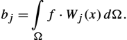
The general term of the system matrix and the right-hand side vector are given by:
aji=∫ΩNi(x)Wj(x)dΩ,
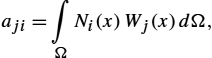
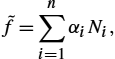
bj=∫Ωf⋅Wj(x)dΩ.
Choosing different base and test functions, respectively, one deals with different approximations of the original functions.
The presented formalism of approximation of functions can be readily applied to the approximate solution of differential equations.
Any differential equation can be considered in the general implicit form of
A(u)=0,
where
A(u)≡L(u)−p.
Therefore, an operator differential equation can be written as
L(u)−p=0,
while the boundary conditions are
M(u)−r=0.
Therefore, the corresponding residuals are given by:
ξΩ=L(˜u)−p,
ξΓ=M(˜u)−r.
And the error due to approximate solution is taken into account by satisfying the fundamental lemma of the variational calculus.
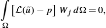
Thus, weighted residual integrals over the domain Ω and boundary Γ vanish, i.e.,
∫Ω[L(˜u)−p]WjdΩ+∫Γ[M(˜u)−r]WjdΓ=0.

In principle, without loss of generality, it is possible to choose base functions to automatically satisfy
M(u)−r=0.
Thus, one has
∫Ω[L(˜u)−p]WjdΩ=0,
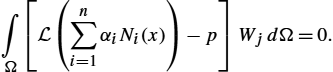
and writing an approximate solution in the form
˜u(x)=n∑i=1αiNi(x),

it follows that
∫Ω[L(n∑i=1αiNi(x))−p]WjdΩ=0.
Finally, an original operator (differential) equation is transformed into a linear equation system:
n∑i=1αi∫ΩL(Ni(x))WjdΩ=∫ΩpWjdΩ,j=1,2,…,n,

which can be written as
n∑i=1ajiαi=bj,j=1,2,…,n,
or in matrix notation,
[a]{α}={b},
where the general matrix term and the right-hand side vector are:
aji=∫ΩL(Ni)WjdΩ,

bj=∫ΩpWjdΩ.
Choosing certain type of base and test functions, one deals with different numerical techniques for the solution of partial differential equations (PDEs).
2.2.2 The Finite Element Method (FEM)
The Finite Element Method (FEM) is one of the most commonly used numerical methods in science and engineering. The method is highly automatized and rather suitable for computer implementation based on step by step algorithms. The special features of FEM are related to efficient modeling of complex shape geometries and inhomogeneous domains, and also to the relatively simple mathematical formulation providing a highly banded and symmetric matrix, same accuracy refinement as by a higher order approximation. The method also provides automatic inclusion of natural (Neumann) boundary conditions. This method generally gives better results than highly robust Finite Difference Method (FDM) approaches [5] in modeling complicated boundaries and is particularly suited for problems with closed boundaries.
2.2.2.1 Basic Concepts of FEM
The calculation domain is discretized into sufficiently small segments – finite elements. The unknown solution over a finite element is expressed in terms of a linear combination of local interpolation functions (shape functions), for 1D problem, as it is shown in Fig. 2.8.

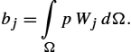
The global base functions assigned to nodes are assembled from local shape functions, assigned to elements, as it is shown in Fig. 2.9 for the case of linear approximation.
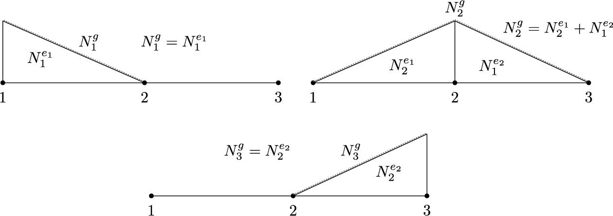
The approximate solution of a problem of interest can be written as
˜f=n∑i=1αiNi,
where coefficients ![]() represent the solution at the global nodes, while n denotes the total number of nodes.
represent the solution at the global nodes, while n denotes the total number of nodes.
The approximate solution along two finite elements is shown in Fig. 2.10.

Elements of local and global nodes and linear approximation of the unknown solution over a domain of interest are shown in Fig. 2.11.

The accuracy can be improved by a finer discretization, or by implementation of higher order approximation.
2.2.2.2 One-Dimensional FEM
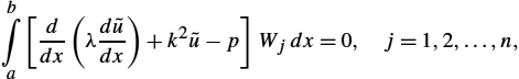
Many problems in science and engineering can be formulated in terms of second-order differential equations of the following form:
where λ and k depend on the properties of a medium and p represents the excitation function, i.e., the sources within the domain of interest. For the one-dimensional case, the domain is related to interval ![]() .
.
Substituting an approximate solution ![]() into the differential equation (2.169) and integrating over the calculation domain according to the weighted residual approach [6], we get
into the differential equation (2.169) and integrating over the calculation domain according to the weighted residual approach [6], we get
which can also be written as

Eq. (2.171) represents the strong formulation of the problem. Within strong formulation, the base functions must be in the domain of the differential operator, and automatically satisfy the prescribed boundary conditions. The strong requirements can be avoided moving to the weak formulation of the problem.
The order of differentiation can be decreased by carefully performing integration by parts. Differentiation of a product of two functions can be written as
Somewhat rearranging Eq. (2.172) and integrating along the interval yields
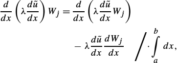
and so one obtains
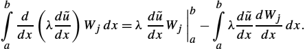
Substituting expression (2.174) into (2.171), the weak formulation is obtained as

The second term on the right-hand side of Eq. (2.175) is the natural boundary (Neumann) condition, thus being directly included into the weak formulation and representing the flux density at the ends of the interval.
Applying the finite element algorithm, the unknown solution ![]() is expanded into a linear combination of basis functions. Implementing the Galerkin–Bubnov procedure (the same choice of base and test functions) yields the following matrix equation:
is expanded into a linear combination of basis functions. Implementing the Galerkin–Bubnov procedure (the same choice of base and test functions) yields the following matrix equation:
where ![]() is the global matrix of the system,
is the global matrix of the system, ![]() is the solution vector,
is the solution vector, ![]() represents the excitation vector, and
represents the excitation vector, and ![]() denotes the flux density.
denotes the flux density.
A local approximation for the unknown function over a finite element is given by
where ![]() and
and ![]() are the linear shape functions.
are the linear shape functions.
Finite element matrix and vector are given by the following integrals:


and the form of the local matrix equation is then

The resulting global matrix system is assembled from the local ones and it is given by

Note that the flux densities vanish at internal nodes, and only the values related to the domain boundary (in the 1D case, interval ends) are not equal zero.
2.2.2.3 Incorporation of Boundary Conditions
Contrary to the Neumann boundary conditions which are automatically included into the weak formulation of the finite element method, the Dirichlet (forced) boundary conditions are incorporated into the matrix system subsequently, i.e.,
thus decreasing the number of unknowns, i.e., the first and last rows of the matrix equations are omitted, and the global matrix equation results in a matrix system of ![]() unknowns:
unknowns:

Once the unknown coefficients, ![]() to
to ![]() , are determined, it is possible from the first and last rows (equations) to obtain the flux densities at the ends of the interval:
, are determined, it is possible from the first and last rows (equations) to obtain the flux densities at the ends of the interval:
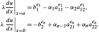
If the Dirichlet condition is prescribed at one end of the interval, and the Neumann condition at the other, then the global system consists of ![]() unknowns and is given by a combination of system (2.181) and (2.183).
unknowns and is given by a combination of system (2.181) and (2.183).
2.2.2.4 Computational Example: 1D Problem
Determine the distribution of time harmonic magnetic field within a slab of length h (h is negligible compared to other dimensions, Fig. 2.12) by discretizing the domain into 2 linear finite elements. The known values are: ![]() ,
, ![]() m,
m, ![]() A/m.
A/m.

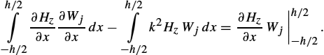
For the 1D wave problem, the time harmonic magnetic field is governed by the following Helmholtz equation:
Applying the weighted residual approach gives

and, having performed integration by parts, one obtains the weak formulation
Now, discretizing the domain to finite elements with Galerkin–Bubnov procedure, ![]() , the general term of FEM matrix is obtained:
, the general term of FEM matrix is obtained:

Provided the linear shape functions are chosen as
the terms of FEM matrix become:

The global matrix, assembled from local matrices, is of the form

and, for the given problem geometry, the global matrix system is given by
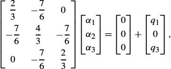
where the corresponding flux densities are:
Finally, inserting the actual boundary conditions gives
and, solving the matrix system
the following value of magnetic field strength is obtained:
Now, the flux densities ![]() and
and ![]() can be determined from the first and third rows of the matrix equation.
can be determined from the first and third rows of the matrix equation.
2.2.2.5 Two-Dimensional FEM
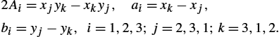
The simplest discretization of a 2D domain can be performed using the so-called triangular elements; see Fig. 2.13. The shape functions are given by equations of planes in 3D space. An approximate solution is shown in Fig. 2.14, while the corresponding shape functions over a triangle are shown in Fig. 2.15. Fig. 2.16 shows the global functions assigned to the ith node, assembled from neighboring shape functions. Note that in the 1D case, global bases always consist of two neighboring shape functions only.


According to Fig. 2.15, the solution on a triangular element is given by
where ![]() ,
, ![]() ,
, ![]() are 2D shape functions determined by:
are 2D shape functions determined by:
Thus, the ith shape function can be written as
where A denotes the area of a triangle,
and ![]() –
–![]() ,
, ![]() –
–![]() and
and ![]() –
–![]() are auxiliary variables:
are auxiliary variables:
or it can be simply written as
Combining relations (2.185)–(2.186c), the solution on a triangle is

where ![]() .
.
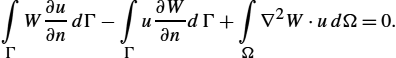
2.2.2.6 The Weak Formulation for Generalized Helmholtz Equation
Many problems in science and engineering can be formulated via the generalized Helmholtz equation. As in the 1D case, FEM is implemented through the weak formulation of the problem.
The generalized inhomogeneous Helmholtz equation can be written in the following form:
where u is the unknown solution, k and r depend on the material properties, while p represents the sources inside the domain of interest.
Applying the weighted residual approach yields
i.e., one obtains

Applying the simple differentiation rule,
and generalized Gauss integral theorem,
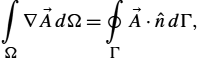
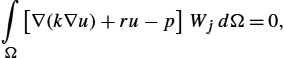
the weak formulation of the Helmholtz equation (2.192) is obtained as
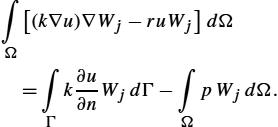
Expression (2.197) is usually referred to as the variational equation [6].
The term on the left-hand side gives rise to the finite element matrix while the first term on the right-hand side is the flux through the part of the domain boundary in which the Neumann boundary condition (flux density) is prescribed. The second term on the right-hand side contains the known sources in the domain if such sources exist.
Applying the finite element algorithm, the unknown solution over an element is expressed in terms of a linear combination of shape functions.
In the matrix form, the approximate solution can be written as follows:

where ![]() denotes the unknown solution coefficients.
denotes the unknown solution coefficients.
The gradient of scalar function u in 2D is simply determined by the relation
Inserting (2.198) into (2.199) yields

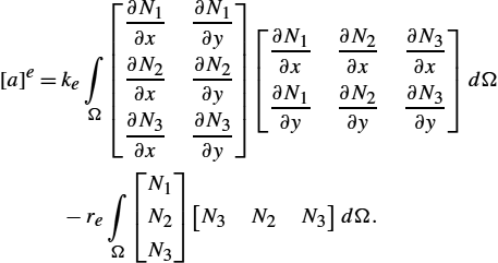
Implementation of the Galerkin–Bubnov procedure (![]() ) leads to the following finite element matrix:
) leads to the following finite element matrix:
Note that it is necessary to discretize the domain into sufficiently small elements thus ensuring the constant quantities over an element. Otherwise, parameters k and r become spatially dependent, which increases the complexity of integration.
The derivatives of shape functions are simply given by:
Performing certain mathematical manipulations yields

The related global matrix is obtained by assembling the contributions from the local ones.
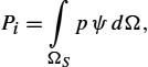
2.2.2.7 Computation of Fluxes on the Domain Boundary
When determining the entire solution for a scalar potential (all coefficients ![]() are known), it is possible to compute
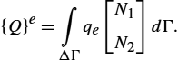
are known), it is possible to compute ![]() , which stem from the potentials. The total flux Q on the part of the domain boundary is defined by the integral
, which stem from the potentials. The total flux Q on the part of the domain boundary is defined by the integral

Quantity ![]() represents the flux density, i.e., the Neumann or natural boundary condition.
represents the flux density, i.e., the Neumann or natural boundary condition.
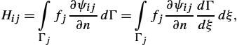
On the finite element located on a part of the boundary, the flux can be expressed by the integral

The flux density q generally varies, but can be assumed constant over an element, provided the element is sufficiently small. Usually, the value of the flux density on the center of the element is taken as the average flux value for the whole element. Note that within the finite element algorithm, the flux Q represents the concentrated value of the flux assigned to the node.
The flux on a finite element located on a part of the boundary can be written as
On the other hand, the concentrated flux on the ith node consists of contributions from neighboring (adjacent) elements, as indicated in Fig. 2.17, is given by the expression
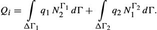
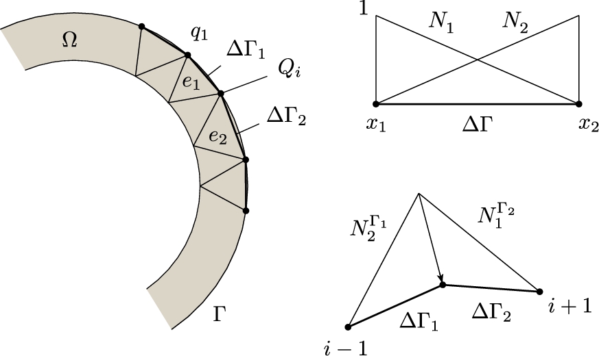
Assuming constant densities ![]() and
and ![]() , one obtains
, one obtains
For the case when ![]() , Eq. (2.208) simplifies into
, Eq. (2.208) simplifies into
For example, if the boundary consists of 3 finite elements with constant flux density, i.e., ![]() , the contributions in nodes are as follows:
, the contributions in nodes are as follows:
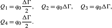
Therefore, only the first and last contributions represent half the value of the other nodes.
2.2.2.8 Computation of Sources on a Finite Element
Contribution of the source on a 2D finite element requires the evaluation of the integral
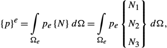
where p denotes the source density inside the domain Ω.
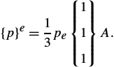
Again, performing sufficiently fine domain discretization, the constant value of the source density over a triangle can be assumed. According to the Galerkin procedure where ![]() , the right-hand side is then
, the right-hand side is then

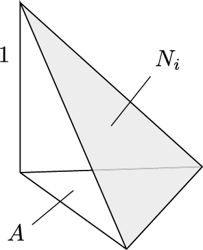
The integral of the shape functions over a triangular element is then

corresponding to the volume of the pyramid with the height equal to 1 and the area of the base (triangle) being A, as depicted in Fig. 2.18.
The right-hand side is now given by the local vector
The assembling of the global system is carried out by using standard FEM algorithm.
2.2.2.9 Three-Dimensional Elements
Similarly as a 2D finite element is constructed from a 1D element, a 3D finite element can be obtained from a 2D element. Thus, by triangle expansion, a three-sided tetrahedral element is obtained, as the simplest 3D element, shown in Fig. 2.19 [20,21].

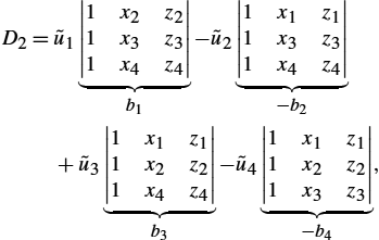
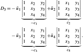
Shape functions can be derived through the same procedure as in the case of 2D triangle elements. The solution on the tetrahedral element is approximated linearly as
Elements ![]() ,
, ![]() ,
, ![]() and
and ![]() are determined from the criterion of function collocation on the vertices of tetrahedron, resulting in the following linear equation system:
are determined from the criterion of function collocation on the vertices of tetrahedron, resulting in the following linear equation system:

Cramer's rule yields
where


Interpolating expressions (2.218)–(2.219d) into (2.217) yields the solution over the considered element:

where the shape functions are
Finally, the solution on the element is expressed as follows:

The derivatives of the shape functions are simply given by:
Note that a consistent order of numbering should be used, often in anti-clockwise direction, as it is indicated in Fig. 2.19.
2.2.3 The Boundary Element Method (BEM)
Since the middle of the 1980s, the boundary element method (BEM) has been used to model a variety of problems in electromagnetics. The basic idea of BEM is to discretize the integral equation using boundary elements [6]. BEM can be regarded as a combination of classical boundary integral equation method and the discretization concepts originated from FEM.
2.2.3.1 Integral Equation Formulation
The first step in solving a problem via BEM is deriving the integral equation formulation of the differential equation governing the problem.
The governing differential equation for the static field problem, either electrostatic or magnetostatic, for source-free domains is defined by the Laplace equation
or the Poisson equation if sources p are present within the domain
A typical calculation domain Ω with the related boundary Γ is shown in Fig. 2.20A, where ![]() is the external normal vector to the boundary, and R denotes the distance from the source to the observation point.
is the external normal vector to the boundary, and R denotes the distance from the source to the observation point.

It is worth mentioning that the observation point P can be also located on the boundary itself, as shown in Fig. 2.20B.
The boundary conditions associated with these problems can be divided into essential condition (Dirichlet), where ![]() , defined on
, defined on ![]() , and natural condition (Neumann),
, and natural condition (Neumann), ![]() , defined on
, defined on ![]() , as shown in Fig. 2.21. The total boundary is then given by
, as shown in Fig. 2.21. The total boundary is then given by ![]() .
.

For simplicity, the case of Laplace equation (2.224) is considered first, and afterwards the procedure can be extended to the solution of Poisson equation (2.225).
Applying the weighted residual approach, Eq. (2.224) can be integrated over the calculation domain Ω:

where W is the weighting function.
Performing some mathematical manipulations and applying the generalized Gauss theorem, Eq. (2.226) becomes
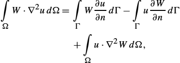
which can be also rewritten as follows:
The weighting function W can be chosen to be the solution of the differential equation, i.e.,
where δ is the Dirac delta function, ![]() denotes the observation points, and
denotes the observation points, and ![]() denotes the source points.
denotes the source points.
The solution of (2.229) represents the fundamental solution, or Green function.
Thus, the domain integral in (2.228) becomes

and, combining Eqs. (2.228)–(2.230), the following integral relation is obtained:
The integral expression (2.231) is the Green representation of function u, where W can be replaced by function ψ.
Function ψ is the fundamental solution of (2.229). For two-dimensional problems, it is given by
while for the three-dimensional case it is
where ![]() denotes the distance from the source point (boundary point) to the observation point.
denotes the distance from the source point (boundary point) to the observation point.
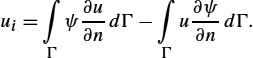
The corresponding Green integral representation of Poisson equation (2.225) can be obtained starting from the weighted residual integral

and performing similar mathematical manipulations, i.e.,
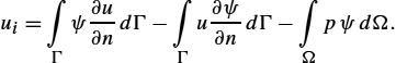
When the observation point P is located on the boundary Γ, the boundary integral becomes singular as R approaches zero. Performing certain procedures to extract the singularity, relation (2.235) can be written as

where

For a well-posed static field problem, either u or ![]() on the boundary Γ must be known, which is described by the forced (Dirichlet), natural (Neumann) or mixed (Cauchy) boundary condition.
on the boundary Γ must be known, which is described by the forced (Dirichlet), natural (Neumann) or mixed (Cauchy) boundary condition.
Knowing all values of potential u and its normal derivative ![]() on the boundary, the potential at an arbitrary point of the domain can be calculated.
on the boundary, the potential at an arbitrary point of the domain can be calculated.
2.2.3.2 Boundary Element Discretization
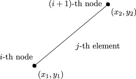
The boundary can be discretized into a series of constant, linear or quadratic elements; see Fig. 2.22.

2.2.3.3 Constant Boundary Elements
The simplest solution can be obtained by using constant boundary elements. The geometry of the constant boundary element for two-dimensional problems is shown in Fig. 2.23.
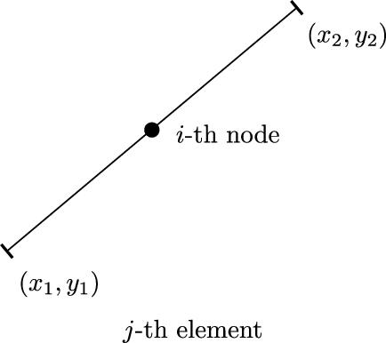
The next step in the boundary element solution procedure is the transformation of the global coordinates into the local ones; see Fig. 2.24.

This transformation of coordinates is given by the following set of ![]() and
and ![]() :
:
where ![]() and
and ![]() are the global coordinates of the element.
are the global coordinates of the element.
In addition, it follows that

where ΔΓ is the segment length defined by
Using the constant boundary element approximation, the integral equation formulation becomes

where i denotes the ith boundary node and j stands for the jth, and p is the constant value of the source on the segment of the domain containing sources.
The resulting algebraic equation system is

or in the matrix form,
where

The matrix system (2.243) can be solved once the set of boundary conditions is prescribed. If the domain of interest contains unknown sources, then a coupling of BEM with some domain discretization method, such as FEM, is required, which leads to hybrid methods.
2.2.3.4 Linear and Quadratic Elements
A higher accuracy and faster convergence can be achieved by applying linear or quadratic elements. Note that the geometry of the elements is also modeled by means or quadratic functions. Such elements are then referred to as isoparametric elements [6]. When using isoparametric elements, the global coordinate x is a function of the local parametric coordinate ξ on the element.
Function x(ξ) can be written as

where approximating functions ![]() are usually polynomials.
are usually polynomials.
Furthermore, the unknowns along elements are interpolated as follows:

where ![]() denotes the unknown coefficients of the potential distribution, and
denotes the unknown coefficients of the potential distribution, and ![]() is the value of the normal derivative at the jth node.
is the value of the normal derivative at the jth node.
Hence, for a linear approximation, it follows that
where ![]() ,
, ![]() ,
, ![]() ,
, ![]() are the values of the vector potential and its normal derivative on the nodes
are the values of the vector potential and its normal derivative on the nodes ![]() and
and ![]() , respectively.
, respectively.
The linear shape functions are given by:
For linear elements (see Fig. 2.25), the geometry is a linear function of the coordinates, i.e.,
For a quadratic interpolation, it follows that
where the shape functions are defined as:
and ![]() and
and ![]() are the values of the vector potential and its normal derivative at the given node j, respectively.
are the values of the vector potential and its normal derivative at the given node j, respectively.
For the case of quadratic elements (see Fig. 2.26), the geometry is represented by following functions:

The resulting matrix equation is
while the corresponding coefficients are now given by

where ![]() denotes the corresponding vector of linear or quadratic shape functions.
denotes the corresponding vector of linear or quadratic shape functions.
The BEM procedures presented so far pertain to the solution of two-dimensional potential problems. If three-dimensional problems are analyzed, then triangular or quadrilateral surface elements have to be applied [19].
2.2.4 Numerical Solution of Integral Equations Over Unknown Sources
The solution of integral equations over unknown sources (indirect boundary element approach) is illustrated on the treatment of Pocklington integro-differential equation (2.131). More mathematical details on the subject can be found elsewhere, e.g., in [6,19]. For simplicity, the integral equation (2.131) can be written in an operator form
where ![]() is a linear operator, I is the unknown current to be found for a given excitation E.
is a linear operator, I is the unknown current to be found for a given excitation E.
The Galerkin–Bubnov Indirect Boundary Element Method (GB-IBEM) of solution starts by expanding the unknown current ![]() into a finite sum of linearly independent basis functions
into a finite sum of linearly independent basis functions ![]() with unknown complex coefficients
with unknown complex coefficients ![]() , i.e.,
, i.e.,

where ![]() is the linear elements shape function, and
is the linear elements shape function, and ![]() stands for the unknown coefficients of the solution,
stands for the unknown coefficients of the solution, ![]() denotes the total number of basis functions. Substituting (2.269) into (2.268) yields
denotes the total number of basis functions. Substituting (2.269) into (2.268) yields
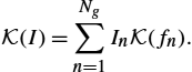
The residual ![]() is given by
is given by

According to the definition of the scalar product of functions in a Hilbert function space, the error ![]() is weighted to zero with respect to certain weighting functions
is weighted to zero with respect to certain weighting functions ![]() , i.e.,
, i.e.,

where ![]() means complex conjugate.
means complex conjugate.
As the operator ![]() is linear, performing some mathematical manipulation and by choosing
is linear, performing some mathematical manipulation and by choosing ![]() (the Galerkin–Bubnov procedure), the system of algebraic equations is obtained:
(the Galerkin–Bubnov procedure), the system of algebraic equations is obtained:

Featuring the weak formulation by carefully performing integration by parts yields
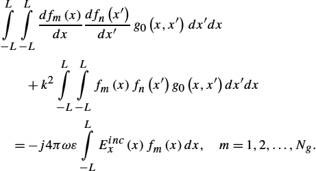
Eq. (2.274) represents the weak Galerkin–Bubnov formulation of the integral equation (2.131). The second order differential operator is replaced by trivial differentiation over basis and weight functions which must be chosen from the class of once differentiable functions.
This formulation is convenient for implementation of GB-IBEM, and boundary conditions are subsequently incorporated into the global matrix of the linear equation system.
Applying the GB-IBEM algorithm and discretizing the wire to segments yields the global system of equations assembled from local ones in a manner similar to finite element step-by-step procedures:

where M is the total number of segments, ![]() is the mutual impedance matrix representing the interaction of the ith source to the j the observation segment, and
is the mutual impedance matrix representing the interaction of the ith source to the j the observation segment, and ![]() is the right-side voltage vector for the jth observation segment.
is the right-side voltage vector for the jth observation segment.
As functions ![]() are required to be once differentiable, a reasonable choice for the shape functions over the segments is the family of Lagrange's polynomials
are required to be once differentiable, a reasonable choice for the shape functions over the segments is the family of Lagrange's polynomials
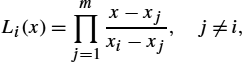
and one has
where ![]() and
and ![]() are the coordinates of the segment nodes and
are the coordinates of the segment nodes and ![]() is the segment length.
is the segment length.
Now ![]() and
and ![]() are given by
are given by
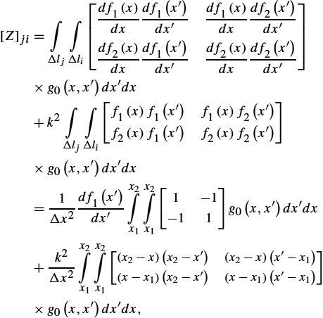
where ![]() represents the right-hand side voltage vector for the jth observation segment,
represents the right-hand side voltage vector for the jth observation segment,

where ![]() ,
, ![]() assign the widths of the ith and jth segments, respectively.
assign the widths of the ith and jth segments, respectively.
The evaluation of the right-hand side vector can be undertaken in closed form if the delta-function voltage generator is used (antenna mode), or the plane wave excitation (scatterer mode). In the radiation mode, the right-hand side vector is different from zero only in the feed gap area. The x-component of the impressed (incident) electric field is given by
where ![]() is the feed voltage and
is the feed voltage and ![]() (for convenience) is the feed-gap width.
(for convenience) is the feed-gap width.
Using the linear shape functions, we obtain

If the scattering mode for the simple case of normal incidence is considered, the wire is illuminated by the plane wave, i.e.,
and then the right-hand side vector differs from zero on an each segment and the local voltage vector is
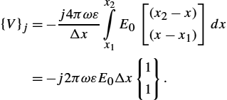
More mathematical details on the method could be found elsewhere, e.g., in [6].
A computational example deals with a classical radiation problem of a dipole antenna radiating in free-space [22] with several applications in computational electromagnetics (CEM).
The wire radius is ![]() mm, operating frequency is
mm, operating frequency is ![]() MHz and length is
MHz and length is ![]() , and 1.25 m which actually corresponds to
, and 1.25 m which actually corresponds to ![]() ,
, ![]() and
and ![]() , where λ is the actual wavelength. The dipole is excited by the unit voltage at its center.
, where λ is the actual wavelength. The dipole is excited by the unit voltage at its center.
Fig. 2.27 shows the corresponding current distribution along the wire.

Once the current distribution along the dipole is obtained, all other parameters of interest could be calculated.