Chapter 3. Describing IPv6
Perfection, of a kind, was what he was after.
Epitaph on a Tyrant, W.H. Auden
In this chapter we’ll cover the features of IPv6 and the basics of its design. This will be a quick tour, addressing the topics of immediate relevance to those using or about to use IPv6. Our intention is to present the information in an easy-to-understand overview format first, and then to get down to the juicy details later in Chapter 4 and Chapter 6.
Designed for Today and Tomorrow
When we talk about networking protocols in general it’s important to understand the difference between specification and implementation. Specifications are written in IETF RFCs and are hotly debated. Implementations are prepared to those specifications, generally by coders or systems people. If you had to choose which one of these to get right, it should of course be the specifications. Broken implementations that misbehave or don’t interoperate can always be rewritten, or even gradually refined; but if your design is inherently broken, you might as well throw away all your work and start again. Since (at the time of writing) we are in a relatively early stage of adoption, we expect that implementation quality will vary across different stacks, but the design is definitely right. Lessons learned during the last few decades of networking have been incorporated into the architecture of the protocol, and so the existing problems with IPv4 have been addressed. In fact, some of the problems with IPv4 will only grow worse over time, and if IPv6 didn’t take them into account, it might flounder even before IPv4 reaches the end of its life.
Perhaps the biggest and most important problem facing IPv4, which will only grow over time, is address space exhaustion.
Address Space Exhaustion
Address space is, with both IPv4 and IPv6, a finite resource. There are only so many addresses that can be allocated from any fixed range. Furthermore it’s a hard limit, pending a change in the meaning of addresses as they are currently understood; one day, you will reach into your “address bag” to assign some new addresses, and there won’t be any more there. Perhaps this won’t be a problem for you immediately—who can say when you might need to grow your network—but it will certainly be a problem for the people you need to communicate with, so it thereby becomes everybody’s problem.
So what’s the scale of this risk? Well, prior to CIDR,[1] IPv4 address allocation, based on class A, B and C addresses, had been over-generous to some users, and address space allocation was running out of control. Today, allocation policies are much stricter, and address space is assigned more frugally. So, the end has not been deferred indefinitely, but the process is definitely under much better control. However, time is inevitably running out: only 36% of the total IPv4 address space remained in 2002, and, depending on whose extrapolations you believe, the remaining space runs out some time between 2005 and 2035. Recent measurements by Geoff Huston suggest that stricter policies have helped considerably, and we may be looking at the upper end of that range. However, even if IPv4 addresses remain available for the next 200 years, but obtaining them requires you to write longer and increasingly baroque essays on why you deserve them, that’s little good to anyone.
Figure 3-1 shows the Internet Systems Consortium’s host count. This count is based on DNS records, which gives data only loosely related to the actual number of live hosts,[2] but does grow proportionally to the amount of address space that has been allocated. We can see that even though growth stalled a little in the last few years, the clock is still ticking.

Optimization
Optimization in this context means two things. First, the design of IPv6 takes into account the problems of IPv4, focusing, in particular, on the consequences for the end user. In other words, the lack of certain desired features is addressed. Management features are one thread in this part of IPv6 tapestry that we choose to isolate for attention. There are serious problems with the way that IPv4 is managed today in enterprises, and IPv6 has the potential to fix those problems. Potential, mind you; no one is pretending that immediate benefits will accrue to any organization implementing IPv6 right now. We shall explain more about this later.
The second aspect of optimization in IPv6’s design is to simplify the mechanisms on which IP is built; for example, the basic IP headers have all been slimmed down to the necessary minimum. This should, in theory, lead to higher performance and lower cost routers, since less processing needs to be done to forward an IPv6 packet than an IPv4 packet. This should also help in areas such as header compression.
Packets and Structures
The IPv6 packet structure is, in most ways, very similar to the IPv4 packet structure. Some fields have been removed and some have been added, but the most obvious change is the size of the addresses. While the IPv4 source and destination addresses are 32 bits each, IPv6 addresses are 128 bits each. The reason for 128 bits is discussed in the following sidebar, Is 128 Bits Enough?
People who remember the second law of thermodynamics (or who have worked in large organizations) know that it is impossible to have a perfectly efficient system. As it is with heat exchangers, so it is with network protocols.
In particular, when addressing endpoints in a real network, from any limited pool, there is a certain amount of the addresses that will be “lost,” or inefficiently allocated. This is not simply due to factors in the protocol itself (for example, wasting addresses on the broadcast address in point to point links) but is also due to real world concerns like administrative error, customer churn, aggregation, and so on. It turns out that this error is actually measurable, and we do it using a metric called the host density ratio, or HD ratio. This is a number that increases from zero to one as the address space fills. For reference, it’s defined as:
Empirical calculations for telephone number allocation and network address assignment show that a HD value of 0.8 is reasonable but a HD value of 0.85 is overcrowded. RFC 3194 goes into more detail.
Having examined common real-world ratios, let’s ask how well can IPv6 do by comparison. One might think that although the size of the address is so much larger, perhaps the inefficiency is larger too, and we might well be back in an IPv4-type address crunch in 10 years time.
Well, let’s look at the numbers. For IPv4 a HD ratio of 0.8 corresponds to 232 * 0.8, or about 50 million hosts. The Internet Domain Survey, http://www.isc.org/ds/, suggests that we passed this point some time ago and are now at a point where HD > 0.85. A comfortable density of 0.8 for IPv6 would correspond to 2128*0.8, or about 1,000 hosts for every gram of the Earth!
We can see that even with relatively mediocre allocation policies, IPv6 can still number all the projected end devices for at least the next few decades. After that, it’s either time for a new protocol, or time to ship people off to another planet (with, of course, a non-bridging firewall).
Basic Header Structure
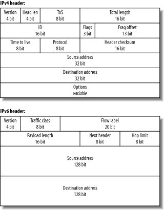
Overall IPv6 actually simplifies the basic header, by including only the information needed for forwarding a packet. This results in a fixed-length header, unlike IPv4. Fixed-length headers are important for router designers and for coders, because it allows more efficient memory allocation strategies and algorithm implementation. Other information, which might traditionally have been stored in the IPv4 header or as IPv4 options, is now stored within a chain of subsequent headers, identified by the next header field. The final header will usually be a TCP, UDP or ICMPv6 header. This way the task of forwarding can be accomplished by dealing with the first few bits of the packet that you have received. Figure 3-2 compares IPv4 and IPv6 headers.
Many familiar fields have equivalents in IPv6: Version, ToS/Traffic Class, Total Length/Payload Length, Time to Live/Hop Limit, Protocol/Next Header, source address and destination addresses. Note the removal of IPv4 fragmentation fields (ID, Flags, Offset), and header checksum. The Traffic Class field is also augmented by the presence of Flow Label field, both used for quality of service, discussed in the Section 3.10 section later in this chapter.
TCP and UDP remain unchanged from IPv4, although individual application protocols that hard-code address sizes may have unpleasant surprises waiting for them in the new world. (We deal with that specific topic in Chapters Chapter 7 and Chapter 8.)
Addressing Concepts
The use of IPv6 addresses is covered in RFC 3513. To begin with, you need to know that IPv6 addresses come in different types (Unicast, multicast, anycast) and different scopes (link, global, and so on). The type of the address determines if packets are destined for one or for many machines. The scope of the address determines which contexts the address makes sense in. We’ll explain more about types and scopes shortly.
RFC 3513 also makes the point that IPv6 addresses are assigned to interfaces on nodes, not to the nodes themselves. This is a big change from IPv4, where very often the address associated with a machine’s interface is that machine. Instead, IPv6 interfaces commonly and usefully have more than one IPv6 address.
In fact, IPv6 allows scoped addresses,
which only have meaning within a certain context. For
example, most interfaces have a link-local address which is only
unique on that specific link. This means that two interfaces on a node could have the
same link-local address if they were attached
to different links! If all of this seems confusing, just think of
the IPv4 loopback address. It is an example of a scoped address
because 127.0.0.1 indicates a
different destination on each host.
Another important concept in IPv6, covered in the RFC, is that of an interface
identifier. In the IPv4 world, we split addresses into a
network part and a host part; an example in CIDR notation is
137.43.0.0/16. In the IPv6 world
the host part is now called the interface ID,
and is used to pick out a particular interface within the specified
network, in the same way that the host part of an IPv4 address picks
out that host on a particular subnet.
The separation has a number of useful properties. Perhaps the most interesting is the potential for automatic assignment of interface IDs. This is one of the nicer features of IPv6, discussed in the Section 3.4.2 later in this chapter. Naturally, manually configuring interface IDs and addresses or using DHCPv6 is still an option, and indeed might be preferable for certain kinds of services.[3]
RFC 3513 also covers the notation used for IPv6 addresses, which we’ll now explain.
Notation
The notation for IPv6 addresses has changed greatly from IPv4. Given a greatly enlarged address space, using or describing IPv6 addresses efficiently becomes much more important than in IPv4, where you are never more than 16 keystrokes from the end of an address. The main differences are outlined below.
Hex digit notation
Instead of ordinary decimal, IPv6 addresses are encoded in hexadecimal, a base-16 numbering
system common in computing and networking. (See the following
sidebar, Decimal, Binary, and Hexadecimal, for more
details). For the moment, it is sufficient to note that the
individual “digits” of an IPv6 address can range not only from
0-9, but also from A-F. Hence an address could begin 2002, for example, and also 20FE or even BD59. Though RFC 3513 uses capitalized
addresses in its examples, IPv6 addresses are
case-insensitive.
Grouping and separation
In IPv4 notation, addresses are “grouped” typographically on octet
boundaries with a dot (.). In IPv6, addresses are grouped
typographically on 16 bit boundaries with a colon (:). Since
addresses are 128 bits long, this means there are 8 groups, every
group using 4 hexadecimal digits. For example, 2001:0DB8:5002:2019:1111:76ff:FEAC:E8A6.
Elision
A lot of IPv6 addresses will contain repetitious elements, particularly zeros. There are ways provided to avoid writing, or elide these in order to speed up the description of these addresses. You can avoid writing all of the elements of an address under the following conditions:
Whenever an address element in a grouping begins with one or more zeros
Wherever there is one or more groups of zeros
In the first case, the leading zeros may be dropped providing at least one
hexadecimal digit is left in the group. In the second case, a run
of groups of zeros may be replaced with a ::. This second elision can only be
performed once, otherwise the address becomes ambiguous.
For example, we can write:
0237:0000:ABCD:0000:0000:0000:0000:0010 |
as 237:0:ABCD::10. How?
First remove the leading zero from 0237. Then remove the leading zeros from
the next group giving 0. Next,
compress the run of zero groups into :: and finally remove two leading zeros
from 0010. We could also have
written the address as 237::ABCD:0:0:0:0:10. Like most things,
reading and writing these addresses gets easier with
practice.
There are certain classes of address space for which it makes sense to return to the old IPv4 ways, but we’ll talk more about those shortly. Suffice it to say that:
::137.43.4.16 |
is also a valid IPv6 address, and could be written:
0000:0000:0000:0000:0000:0000:892b:0410 |
Example 3-1 shows some perl code that uses these rules and expands IPv6 addresses to their full form. Example 3-2 shows example inputs and this program which you might want to compare to the expanded forms in Example 3-3 to see this compression in action.
#!/usr/local/bin/perl

while(<>) { print &expandv6($_), "
"; }

sub expandv6 {
        local ($_) = @_;
        local (@parts, @newparts, $part);

        s/s+//g; # Get rid of white space.
        s/%.*//g; # Get rid of MS/KAME scope ID, if there is one.
        if (/:(d+).(d+).(d+).(d+)$/) { # Expand trailing IPv4 address.
                $part = sprintf ":%02x%02x:%02x%02x", $1, $2, $3, $4;
                s/:d+.d+.d+.d+$/$part/;
        }

        @parts = split(/:/, $_, -1);
        $short = 8 - $#parts;
        @newparts = ( );

        foreach $part (@parts) {
                if ($part eq "" && $short >; 0) {
                        while ($short-- >; 0) { push @newparts, "0000"; }
                } else {
                        push @newparts, (sprintf "%04x", hex($part));
                }
        }

        return join ":", @newparts;
}

1;:: 237:0:ABCD::10 ::137.43.4.16 2001:770:10:: ::0 ::ffff:0.0.0.0 200:: 2000:: fe80:: fec0:: ff00:: 2001:1200:: ff05::1:3 ff02::1:ffab:cdef ff02::2 fe80::134.226.81.10 2001:770:10:300::134.226.81.11
0000:0000:0000:0000:0000:0000:0000:0000
0237:0000:abcd:0000:0000:0000:0000:0010
0000:0000:0000:0000:0000:0000:892b:0410
2001:0770:0010:0000:0000:0000:0000:0000
0000:0000:0000:0000:0000:0000:0000:0000
0000:0000:0000:0000:0000:ffff:0000:0000
0200:0000:0000:0000:0000:0000:0000:0000
2000:0000:0000:0000:0000:0000:0000:0000
fe80:0000:0000:0000:0000:0000:0000:0000
fec0:0000:0000:0000:0000:0000:0000:0000
ff00:0000:0000:0000:0000:0000:0000:0000
2001:1200:0000:0000:0000:0000:0000:0000
ff05:0000:0000:0000:0000:0000:0001:0003
ff02:0000:0000:0000:0000:0001:ffab:cdef
ff02:0000:0000:0000:0000:0000:0000:0002
fe80:0000:0000:0000:0000:0000:86e2:510a
2001:0770:0010:0300:0000:0000:86e2:510b
Scope identifiers
As mentioned in the Section
3.2.2 earlier in this chapter, IPv6 allows scoped addresses
which are only meaningful in a particular context. The most common
of these addresses is the link-local address, which is only
meaningful on a particular network link. Suppose you want to ping
a link-local address like fe80::1, and your computer is connected
to several links. The address fe80::1 could be on any one of those
links, so how does IPv6 know which one to use?
One way to solve this problem is to add a flag to programs
like ping, to allow the
specification of an interface. For example, the KAME and Microsoft
stacks allow the specification of link as part of the address, by
including a scope identifier. On a
KAME-derived stack, as found on BSD systems, fe80::1%en0 means the address fe80::1 on the network attached to
interface en0. On Microsoft
derived stacks the scope-id is usually given as a number, so
fe80::1%7 means address
fe80::1 on IPv6 interface
7.
Subnetting
In IPv4, subnetting allows you to
take pieces of your existing address space and divide
it, to provide either more networks or to make more addresses
available to certain people. One common example of using subnetting
to provide more networks is an ISP assigning a subnet of their
address space to a customer. An example of using subnetting to make
more addresses available is when a company finds that its sales team
have run out of addresses, but R&D have some spare. If R&D
are using less than half of the 256 addresses in their /24 say, then a /25 could be reclaimed and assigned to
sales.
IPv6 can subnet too. It uses the CIDR notation developed for IPv4 as well, which is a way of
specifying the size of a network in addition to the actual network
number. An example from IPv4 is 137.43.0.0/16, which is the old “class B”
network of University College Dublin. Similarly, 2001:770:10::/48 is the IPv6 network of
Trinity College Dublin. In IPv6 these blocks of addresses are often
referred to as prefixes. Single hosts in IPv4 are called /32’s, and
consequently single hosts in IPv6 are /128’s. (A calculator that can
do CIDR calculations on IPv4 and IPv6 addresses is available at
http://www.routemeister.net/projects/sipcalc/;
you might find it useful for getting up to speed on IPv6 network
numbering.)
In IPv6, subnets are supposed to be at least 64 bits wide,
even for point-to-point links. Since an individual /64 has space for over a billion hosts, it
is expected that re-subnetting to provide more addresses for an
individual network will no longer be necessary. This is an important
point: possibly the best way to understand it is to take the example
of an IPv4 server farm that has outgrown the 256 addresses (only 254
of them being usable of course) in its /24. With IPv4 you have no choice but to
subnet, creating another piece of network either contiguous or
discontiguous to the original addresses, and add your new servers
there, with consequent impact on the routing within your
organization. In contrast, with IPv6, since the servers can all have
a different interface ID, they can all live in the same subnet. This
would allow large groups of machines, say Beowulf clusters, to
happily fit within any subnet.
Therefore, the main reason for subnetting becomes the
assignment of networks for different administrative or technical
purposes, such as security or routing. To try to simplify this
process, it is expected that organizations requiring internal
subnetting will always be assigned a /48.[4] This means that everyone has 16 “network” bits to work
with, or 65536 different subnets. This should be enough for
anybody.[5]
Address Architecture
Those of you who are familiar with IPv4 networks may have encountered the notion of private versus public address space. Private address space is address space used within an organization’s network, and in theory it cannot be reached from the outside world (often people like to pretend that this gives them additional security, see “NAT” in Chapter 1). These addresses are an example of address spaces with special properties—and often (but not always) these types of address space can be inferred by glancing at the address.
Examples of special addresses from the IPv4 world include the
private class A space 10.0.0.0/8,
which is discussed in the “Addressing Model” section in Chapter 1, and would be familiar to
those building enterprise networks. Similarly 127.0.0.0/8 is the “localhost” space, which
hosts use to contact themselves.
Warning
One interesting IPv4 special address is the “broadcast” address in IPv4, 255.255.255.255, because it has no direct equivalent in IPv6. Broadcasts no longer exist in IPv6, and multicast is used as the transport for contacting multiple hosts simultaneously.
Similarly in IPv6 there are a number of address spaces, usually expressed as a prefix with CIDR network length. The official breakup of this space is documented on the IANA web site http://www.iana.org/, but we summarize the allocations in Table 3-1.
Prefix | Intended use |
| Unspecified/loopback/compatible-IPv4 address |
| Mapped IPv4 addresses |
| Reserved for NSAP Allocation (RFC 1888) |
| Reserved for IPS Allocation |
| Global Unicast (RFC 3587) |
| Link-Local Unicast |
| Site-Local Unicast (deprecated in RFC 3879) |
| Local IPv6 Unicast addresses (proposed) |
| Multicast |
A few of these types of addresses are worth explaining in more detail.
Global Unicast Addressing
These addresses are the analogue of the normal public IPv4 address space. Most of these addresses are still reserved, but the allocation of this space to users has begun. The blocks that have been allocated are listed in Table 3-2.
Prefix | Intended use | RFC |
| Production via Regional Internet Registries | RFC 2450 |
| 6to4transition mechanism (see Chapter 4) | RFC 3056 |
| 6bonetest network | RFC 2471, RFC 3701 |
Some of the production address space is being allocated to Regional Internet Registries[6] in large chunks. The RIRs are in turn then responsible for allocating smaller blocks to Local Internet Registries, who are usually Internet Service Providers. Finally, ISPs assign addresses directly to their customers.
This hierarchical address allocation scheme is expected to be the normal way that end users get IPv6 addresses.
Link-Local Addressing
The link-local prefix contains addresses that are only meaningful on a
single link. In fact, this prefix is used for on almost
every link that IPv6 is configured on. This
means the link-local address fe80::feed will refer to a different
computer depending on which network you are using, much like
127.0.0.1 refers to a different
computer depending on which one you’re using.
In this context, a link is a group of machines who may communicate directly without requiring an IPv6 router. This link may be a point-to-point, a broadcast link or something more esoteric, but packets addressed using link-local addressing will never pass through a router.[7] Addresses that are only valid on the local link may not seem very useful, but they form a part of the IPv6 autoconfiguration process.
It’s important to note that hosts generate link-local addresses by virtue of being connected to a link; no router or involvement by any outside agency is necessary for these addresses to be generated and used. So, a small office with one switch and a few computers connected can use link-local addressing for simple networking.[8] This is one of the major contributions of IPv6 to ease of management, especially for small organizations. (We’ll get to how link-local addresses are actually generated in a moment.)
It is also possible to use link-local addresses when “real” addresses are not strictly required. For example, a point-to-point link between two routers could operate with only link-local addresses, without having to allocate any global Unicast addresses. However, IPv6 has been designed so that there should be no shortage of addresses and this sort of address conservation should be unnecessary. Also, routers may require real addresses for sending ICMP error messages or for remote management.
Automatically configured link-local addresses are in some ways
quite similar to the IPv4 169.254.0.0/16 addresses that are
sometimes used if no DHCP server is available or if only link-local
communication is required. IPv6 autoconfigured addresses differ here
in that they are intended to be unique and constant, whereas the
IPv4 addresses are prone to collision and may vary as a consequence
of collision resolution.
Site-Local Addressing
Site-local addressing is an interesting idea somewhat reminiscent of the IPv4 private address spaces discussed above. These addresses are meant to be used within a site,[9] but are not necessarily routable or valid outside of your organization. Opinions vary as to the definition of a site, but think of it as being an organization to which an address space allocation might be made. The reason for this is that as the use of site-local addressing mirrors the use of global addressing, it should simplify management of addresses and encourage sensible use of both.
Unlike link-local addresses, which are only required to be unique on a link, these site-local addresses require a router to be configured to avoid duplication of site-local addresses within a site.
At the moment the practical details of if and how site-local addressing should be deployed are still being discussed. There is a general wish to avoid the sort of problems associated with merging private networks (as discussed in “NAT” in Chapter 1). What this probably means is that there will be “site-local” addresses that are globally unique. However, it seems that site-local addresses, as originally considered for IPv6, have been abandoned and the details of this new “unique local IPv6 Unicast addressing” are being finalized. Given the clear need for stable in-site addressing in the face of provider allocated global addresses, considerable effort is being invested in getting the replacement for site-local addresses right. (We’ll comment more on the future of site-local addresses in Chapter 9.)
Enough address space has actually been dedicated to site-local and unique local addressing to assign unique addresses to most organizations in the world. Thus it is possible that these addresses could actually end up being globally valid and routable! The main problem with this is that it is not clear how to solve the technical problems associated with routing such a large, unstructured address space.
For now, the best thing to do with local addressing is to ignore it. Once its future is clearer it may be useful to some people, but for now most people can survive with a combination of link-local and global addressing.
Multicast
Let’s consider applications where conversing with many hosts at once is the norm. How can you make this happen as efficiently as possible? Unicasting data to many hosts is inefficient, because you have to send the data once for each host. Broadcasting to many hosts is also inefficient, because many hosts will not be interested in the data you are sending, and will waste resources processing the packet. Multicast is the solution allowing you to send a packet efficiently to an arbitrary collection of machines. It aims to be a compromise between Unicast and broadcast; hosts can sign up to receive messages destined to specific groups, and these multicast groups are identified by multicast addresses.
The usual example of a multicast application is streaming multimedia; lots of end stations need to receive the same rock video/party political broadcast from a single source. From an application point of view you send packets to a single group address, but everyone who has registered as being in that group receives the data. Naturally this requires the cooperation of routers and switches within the network.
Multicast exists in the IPv4 world; IGMP, defined in RFC 3376, is used to manage IPv4 multicast groups. However, multicast, although useful, has never really had wide deployment. By contrast, in IPv6, multicast is compulsory. Indeed, multicast is central to the operation of IPv6; IGMP has been merged into ICMPv6 (RFC 2710) and multicast is used to implement IPv6’s equivalent of ARP. We talk more about this in the Section 3.4 section later in this chapter.
Multicast requires no configuration if it is confined to a single network (i.e., a single link). However, for multicast traffic to cross routers a multicast routing daemon must be configured. For now we’ll concentrate on link-local multicast.
Multicast addressing in IPv6
The IPv6 multicast address space described in Table 3-1 is split up into
into chunks mirroring the different types of Unicast addresses.
Multicast addresses are of the form ffXY:... where X is 4 bits of flags and Y is the scope of the multicast.
The top bit of the flags are currently reserved and should be zero. The final bit is 1 if the multicast address is a transient multicast address, rather than a well-known one.[10] For well-known addresses the other flags must be set to 0, the other values being reserved for later use.
The situation for transient addresses is a little more complex, but we only need to review it briefly. Here the value of the two middle flags is important. A middle flags value of 00 indicates an arbitrary assignment of addresses, where the addresses are assigned by those operating the link/site/network matching the scope of the address. Middle flags of 01 indicates assignment based on Unicast prefix, where by virtue of using a block (prefix) of IPv6 addresses, there is automatically a block of IPv6 multicast addresses available. Finally, middle flags of 11 is another assignment based Unicast addresses, but this time the address of a rendezvous point is also encoded in the multicast address. A rendezvous point is a place in a multicast network that acts as a distribution point for a particular multicast stream. Locating a rendezvous point is a tricky problem in some types of multicast routing, so including it in the address makes life easier.
The scope values are shown in Table 3-3, as are prefixes for well-known and simple transient addresses with this scope. There are similar blocks of addresses for the other flags values too.
Scope | Value | Well-known | Transient |
reserved | 0 | | |
node-local | 1 | | |
link-local | 2 | | |
site-local | 5 | | |
organization-local | 8 | | |
global | E | | |
reserved | F | | |
Within each of the well-known ranges, some addresses have
been assigned for specific uses. Some assignments are variable scope, meaning
that they are assigned for any valid scope value. For example,
ff0X::101 is assigned to NTP
servers with scope X.
Other assignments are only valid within certain scopes, for
example DHCPv6 servers are assigned the site-local scope address
ff05::1:3.
In some cases, ranges of addresses have been assigned. In
particular, ff02::1:ff00:0/104
is the range for solicited node multicast.
If a node has a Unicast address ending in, say ab:cdef, then it must be part of the
multicast group ff02::1:ffab:cdef. Since an interface
can have several Unicast addresses, this may mean several
solicited node multicast addresses on that interface. However, if
the interface ID is the same for all the Unicast addresses, then
the interface will only need to join one solicited node multicast
group.
The list of assigned multicast addresses is available on the
IANA web site http://www.iana.org/, and is relatively
long. However, there are two multicast address everyone should
know about: ff02::1 and
ff02::2. The first is the
link-local all-nodes address, the rough equivalent of the
non-routed broadcast address 255.255.255.255 in IPv4. The second is
the link-local all-routers address, which is important in the IPv6
autoconfiguration process.
Hardware support
One final thing to note is that some sort of support is required in the end
networks to support multicast. For example, in Ethernet networks
certain destination MAC addresses are set aside for multicast. For
IPv6 these addresses have the two high bytes set to 33:33 and the remaining four bytes taken
from the low four bytes of the IPv6 multicast address.
This means that to receive multicast you need an Ethernet card that can pass up packets addressed to the relevant layer two address. Modern cards often have a facility called multicast filters, which allow only relevant multicast packets to be passed up to the driver, which means that the driver can avoid processing every multicast packet that the card receives.
If the card doesn’t have this hardware support, the necessary filtering can be done in the Ethernet driver. Some hosts may actually want to receive all multicast packets. This is implemented with multicast promiscuous support that passes up all Ethernet frames that have a multicast destination address. If your Ethernet driver has to process all multicast frames, either because it does not support multicast filters or because it is operating in multicast promiscuous mode, it will obviously consume more of the computer’s resources.
All this configuration of Ethernet multicast filters should automatically be done by the IP stack and Ethernet drivers, so you shouldn’t have to worry about it. However, occasionally it doesn’t work. We talk about what can go wrong with Ethernet multicast support in Section 5.7 of Chapter 5.
Anycast
An anycast address is an address half way between a Unicast address and a multicast address. Unicast addresses are assigned to one machine and each packet is delivered to that machine. Multicast addresses are assigned to many machines and each packet is delivered to all such machines. Anycast addresses are assigned to many machines, but each packet is delivered to only one of these machines. The use of anycast is still settling down, so we discuss it in Chapter 9.
ICMPv6
TCP and UDP have both remained unchanged from IPv4 to IPv6. ICMP is a very different story, as ICMPv6 encompasses the roles filled by ICMP, IGMP and ARP in the IPv4 world. Some aspects of ICPMv6 will be familiar to those who have worked with their IPv4 equivalents: ICMP Echoes and Errors, for example. However, the most important changes are in the area of neighbor discovery, which will be unfamiliar to IPv6 newcomers. We discuss this in the Section 3.4.2 section later in this chapter.
ICMP Echoes and Errors
RFC 2463 covers the part of ICMPv6 that is most similar to the familiar parts of ICMPv4. It covers ICMP Echo Requests and Replies, which are used to implement the well-known ping program. It also covers ICMP errors, which are returned when there is a problem with a packet: Destination Unreachable (because of routing, packet filtering or other unavailability), Packet Too Big, Time Exceeded (when the packet has travelled too many hops) and Parameter Problem (unknown or bad headers).
ICMP messages have often been filtered out in the IPv4 world, which usually results in the failure of tools such as ping and traceroute or delays while waiting for the arrival of discarded “destination unreachable” messages. IPv6 will be even less forgiving in this respect, as correctly operating ICMP is absolutely essential to the protocol. In particular, Packet Too Big messages are now necessary for the valid operation of TCP and UDP because IPv6 routers are not permitted to fragment packets. Nodes need to be told to reduce the size of a packet if it will not fit within the MTU of a link. The process of figuring out the largest packet that can be sent to a particular destination is called path MTU discovery. IPv6 path MTU discovery is described in RFC 1981. IPv6 nodes are not required to use path MTU discovery, but if they don’t, they must not send packets larger than 1280 bytes, the minimum permitted IPv6 MTU.
ICMP error messages are also explicitly rate-limited by the stack. This will usually restrict the number of error messages sent either per-period-of-time or to a fraction of link bandwidth (there are details of some suggested schemes in RFC 2463). This avoids repeating some mistakes IPv4 made with respect to overzealous, or overly-compliant, ICMP message generation.
Neighborhood Watch
Address resolution in IPv4 uses ARP, but in IPv6 a mechanism known as neighbor discovery is used. Neighbor discovery also provides additional features that are not provided in IPv4. Neighbor discovery is defined in RFC 2461.
Unlike ARP, ICMP neighbor discovery is an IP protocol, which means that it can be secured with IPsec (the Section 3.9 later in this chapter introduces IPsec). As a precaution, most neighbor discovery packets are also only acted on if they have not been forwarded by a router. This is achieved by checking the hop-limit field has its maximum value and makes it difficult to inject them into remote networks.
Like ARP, neighbor discovery explicitly includes the link-layer addresses within the body of messages, rather than peeking at the packet’s link-layer header. This makes for easier implementation and also leaves the option of proxy neighbor discovery open for situations such as Mobile IP.
Address resolution
Neighbor Solicitation and Neighbor Advertisement are two types of ICMPv6 neighbor discovery packets. They have several uses, but the one that we will mention here is the equivalent of ARP in IPv4.
A neighbor solicitation packet is very similar to an ARP request packet. It is sent when a node wants to translate a target IPv6 Unicast address into a link-layer address. Basically it says, “Can the owner of this IPv6 address please get in touch?” Since we don’t actually know the link-layer address of the target host, the neighbor solicitation packet is sent to the solicited-node multicast address[11] corresponding to the target address, and the target address is included in the ICMP message. The sending node will also usually include its link-layer address, to make replying easier.
A neighbor advertisement packet is the logical response to these solicitations. It is sent back to the requesting system, including the source address of the solicitation, the link-layer address of the target system and some flags.
An example of neighbor solicitation between two hosts is
shown in Figure 3-3.
Host 1 wants to talk to address 2001:db8::a00:2 on host 2, so it
calculates the solicited node multicast address ff02::1:ff00:2 and sends the packet to
the corresponding Ethernet multicast address. It includes its own
Ethernet address in the packet. Host 2 responds with a neighbor
advertisement sent directly to host 1’s Ethernet address.

In the same way that hosts had an ARP table in IPv4, there is a table of neighbors maintained on a node in IPv6 called the neighbor cache. This cache manages the results of previous queries to avoid repeating requests too often.
Unlike ARP, ICMPv6 avoids broadcasts. The use of a whole range of solicited node multicast addresses means that nodes will usually only have to process Neighbor Solicitation packets that are actually of interest to them. This means that the interrupt load on IPv6 hosts should be much lower than on the equivalent IPv4 network.
DAD
Duplicate Address Detection (DAD) is a feature which is useful for network operation. It is used when an address is assigned to an interface and is a way of checking that no node on the link is already using that address. It can be used for any address type (e.g., Unicast or link-local) but can only detect duplicates that share a link with you. DAD is defined in RFC 2462.
When an interface is manually or automatically configured, the address is marked as tentative. The Duplicate Address Detection procedure then sends a Neighbor Solicitation message to the address that has just been configured. The idea is simple: you wait a certain amount of time, and if you have not received a reply, then you conclude the address is not in use and proceed merrily on your way. If you do receive a reply, it is in the form of a Neighbor Advertisement, so you mark the tentative address unusable and operator intervention is required.[12]
The Neighbor Solicitation message is addressed to the appropriate solicited-node
multicast address, and the address that is being checked as unique
is sent as the target. Since we do not want to use the tentative
address yet, the source address is set to the all-zeros
unspecified address ::. If a
node replies to such a solicitation, the advertisement must be
sent to the all-nodes link-local address ff02::1 because the host doing DAD may
not yet have any addresses. If a duplicate address is discovered
then the tentative address must not be used.
Unfortunately DAD is not a completely reliable mechanism; you might wait a long time but not long enough, or the reply could be lost or discarded for a variety of reasons. Compared to IPv4, DAD is a better approach to minimizing the chaos that ensues when addresses are unwillingly shared. If nothing else, mandatory DAD helps you as an innocent bystander and hinders you as a malicious attacker!
NUD
A host can fall off a network at any time, with reasons ranging from sudden power loss to malicious intent. Neighbor Unreachability Detection is a way of checking that we are still in bidirectional contact with a neighbor. Usually this can be inferred by what RFC 2461 refers to as “forward progress” of a high level protocol, such as TCP. However, if a neighbor seems to have gone missing, a Neighbor Solicitation can be sent to them to see if they are still available.
What good is determining if a neighbor has become unreachable? Well, in the case where the neighbor has become unreachable because of a change of layer 2 address (perhaps because of some hot-standby system), the Neighbor Solicitation will then discover the new layer 2 address corresponding to the original IPv6 address. If the system that has become unavailable is a router, then we may be able to choose another router. In cases where the unreachable neighbor was an end-host that has been powered off, then there probably isn’t much we can do to restore useful communication.
Redirection
As in IPv4, sometimes a node makes a bad decision about the best router to receive a particular packet. Again, as with IPv4, a router can signal to a host and indicate a better choice of next hop. IPv6 does add some extra features to ICMPv4 redirection; it can indicate the link-layer address of the next hop and can let a node know that an address thought to be remote is actually local. One quirk of IPv6 redirection is that redirection uses link-local addresses, which means that routers need to know one another’s link-local addresses.
Router/prefix advertisement
The remaining two packet types in the neighbor discovery suite are the Router
Solicitation and Router Advertisement packets. Router
solicitations are like neighbor solicitations, but rather than
asking about other nodes, they are seeking information from local
routers. Consequently, these are sent to the all-routers multicast
address ff02::2.
Router solicitations are not strictly necessary, as router advertisements are sent automatically every so often. For example, a laptop that awakes from hibernation might not send a router solicitation, but it could refresh the prefix information after a few minutes when the router next sends an advertisement. The time between these announcements is configurable, but is usually randomized to prevent undesirable synchronization effects.
Router advertisements contain all sort of useful goodies that a host may want to know about: prefixes, link MTUs, and so on. Unless you are anxious to preserve the practice of manual configuration in your network, the router discovery mechanism will be the primary mechanism by which default gateways are learned for hosts. Essentially a host has to do very little other than listen to quasi-periodic announcements to configure itself. The announcements are issued per router per link. Each announcement contains information about the specific address prefixes that the host can contact on this link. Some of these prefixes may be marked as suitable for use in autoconfiguration. Router advertisements also indicate that the router is available as a default router to hosts on the link, and may even carry information about what routers are close to specific prefixes.
How does a host resolve the problem of hearing about multiple routers? In the absence of the routers advertising specific routing preferences, a host can pick any suitable router. Redirection and Neighbor Unreachability Detection will ensure that the traffic is directed in the correct way.
There are a number of parameters that enable the router administrator to influence the behavior of hosts who receive the messages. They can:
Specify that hosts must do stateful autoconfiguration (e.g., DHCPv6)
Specify that hosts must do stateless autoconfiguration
Specify the link MTU
Specify the default hop limit
Specify the length of time for which hosts are considered reachable
From the network managers’ point of view, it is very useful to be able to control parameters like this centrally and with so little effort. This is part of why IPv6, when properly deployed, should save us money and time.
Of course there are security tradeoffs—if you were a host on a network, and able to fake router advertisements, the fun things you could do range from nasty but traceable (advertising the prefix for some important web site) to nasty and impossible to guess (changing the hop limit to two or three so that connecting to local servers would succeed, but long range connections would fail mysteriously). Again, because all this takes place at the IP layer, in principle it can be secured with IPsec, however key distribution issues make this tricky. In light of this, a secure neighbor discovery protocol called SEND has been proposed for networks where untrusted nodes are connected. In IPv4 there are simply no complete solutions to this kind of problem.
Stateless autoconfiguration
Stateless autoconfiguration is a long name for an extremely desirable thing: being able to get devices working—hence, configuration—without any manual intervention—hence, auto—and without requiring server infrastructure to support it—hence, stateless.
This is to contrast it with stateful autoconfiguration, exemplified by protocols such as DHCP. DHCP is extremely useful and is very flexible about delivering information that a host requires to use network resources, but it requires a server and someone to maintain it, and these are not things that every deployment of computers can expect to have—or indeed should need to have.
In stateless autoconfiguration on Ethernet, a host uses the following pieces of information:
MAC addresses
Network prefixes
in order to generate valid addresses.
To form the complete set of addresses, a host first applies a rule, which we describe below, to the MAC address of each of the network interfaces it has. MAC addresses are of course, unique, and it is this property which makes autoconfiguration as practical as it is. (If the uniqueness of the addresses were in question, then a host could just randomly formulate an address, but the lack of a tight coupling between node and address would create havoc for network managers. In fact, the use of the MAC address, which may be tied to a removable Ethernet card rather than the node itself, is one of the downsides of the scheme.)
The rule that is applied transforms the MAC address into an
interface ID is shown in Figure
3-4. It works in the following way. Suppose you have a MAC
address on your Ethernet card of 00:50:8B:C8:E6:76. First, the seventh
bit of the address (which is defined by the Ethernet standard to
be the “universal/local” bit), is set giving 02:50:8B:C8:E6:76. Then this is split
into two halves, 02:50:8B and
C8:E6:76. Finally, FF:FE is inserted between them. In this
case it would form 02:50:8B:FF:FE:C8:E6:76.

These 64 bits are called an EUI-64 identifier, after the
globally unique IEEE identifier, and are used as the interface
identifier in stateless autoconfiguration. Initially, the
link-local prefix fe80:: will
have these 64 bits appended to form a tentative link-local
address.
These newly-formed addresses, once they are tested for duplication via DAD, can thereafter be used for network communication with the node’s neighbors. When router advertisements are received, the host can perform the process of concatenating the advertised prefixes with the interface identifier to produce other addresses. Thus link-local addresses can be generated without any connection to the outside world—perfect for an accountant’s office, or other small-office/home-office scenario where internal network resources are more important. In this situation, name resolution can be done via broadcasts or similar mechanisms that do not require Internet access or a server. (Addressing in networks containing more than one link is more complex and really requires either global addresses or unique local addressing.)
The advertisements of prefixes also include information to say how long the prefix is valid for. As long as the router continues to re-advertise the prefix, then the address will remain valid. If a router stops advertising a prefix then the address can become deprecated after the prefix’s valid lifetime elapses. Deprecated addresses can still be used, but other addresses are preferred for new communication. For this reason, addresses that have not been deprecated are sometimes called preferred addresses.
It is important to understand that the address generation ability of stateless autoconfiguration does not have to be invoked unless the administrator, should there be one, decides so. Some people, upon hearing of the mechanism, imagine it being applied to their servers and firewalls and so on, and the thought of them changing addresses arbitrarily if a network card fails and has to be replaced is unsettling. Thankfully, addresses in IPv6 can be statically defined just as IPv4 addresses are today, and neighbor discovery will take care of everything.
Privacy is another concern raised by autoconfiguration. If a laptop moves from network to network, using autoconfigured addresses, it will use the same interface ID on each network. This could allow the tracking of that laptop as its owner moves from work, to home, to the airport and so on. RFC 3041 proposes a extension to autoconfiguration where extra temporary addresses are generated, which can be used for outgoing connections to preserve the users privacy. These addresses are generated using MD5 and some random data associated with the node, and are disposed of periodically to make tracking impractical.
ICMP name resolution
There is a proposed mechanism for doing discovery of node names and addresses using ICMPv6. The usual mechanism for this is, of course, DNS. However, the IPv6 mechanism provides for name translation in serverless networks and also allows the querying of all of a node’s addresses without having to hope that DNS is up to date or, indeed, in use at all.
The mechanism involves a Node Information Query packet, which can ask for the names or IP addresses of a node and a Node Information Reply packet, which is the corresponding response. These queries can be directed to any node, not just your neighbors, but a node can choose not to provide information if it wishes.
It also defines a new set of link-local multicast groups
ff02::2:0:0/96, known as the
node information groups. This allows a node to efficiently query
the names and addresses of all nodes with a particular name
without sending a broadcast, by calculating the correct multicast
group based on a hash of that name.
The standardization of node information queries isn’t in the near future, however a number of stacks implement it and it seems to be working well on KAME-derived implementations.
Router Renumbering
Autoconfiguration of IPv6 addresses makes it relatively simple to change the addresses assigned to groups of machines, by changing the prefixes advertised by routers. This reassignment of address is commonly referred to as renumbering. Hosts are easy, but what about routers themselves? An automatic way to renumber these also is required, since otherwise large networks[13] would require significant manual intervention to renumber anyway. Thankfully RFC 2894 provides a solution to the problem.
RFC 2894 defines a router renumbering ICMP message. These messages act like a search-and-replace operation on the existing prefixes used by the router, and can also change parameters like the prefix lifetime. The three operations that can be performed are ADD (adds new prefixes based on matching existing prefixes), CHANGE (adds new prefixes, but also deletes existing matching prefixes) and SET-GLOBAL (like change, but removes all global scope addresses, rather than just matching ones). Each of these operations can match a single prefix and produce several new prefixes from it.
To take an example, suppose we are moving a customer from the
prefix 2001:db8:dead:/48 to
2001:db8:babe:/48, but otherwise
want to leave the structure of their network intact. We first send a
message to all routers, telling them that if the router has a prefix
2001:db8:dead:XXXX/64, then to
add a new prefix 2001:db8:babe:XXXX/64, where the XXXX bits are copied from the old prefix
to the new one. Then we can send a message to shrink the lifetime
associated with prefixes under 2001:db8:dead:/48, so deprecation will
occur more quickly. Finally, we can send out another change request
to remove all prefixes under 2001:db8:dead:/48.
Router renumbering has serious implications for security, so updates need to be authenticated with IPsec. Furthermore, for ease of operation it would be desirable to have the site-local all-routers address listening for updates. Of course, while router renumbering provides a good way to renumber the routing infrastructure, it doesn’t obviously extend to renumbering servers that may have manually configured IPv6 addresses on interfaces or stored in configuration files. These factors mean that renumbering is not as simple as one would like in the IPv6 world.
Multicast Listener Discovery
Most of the aspects of multicast that we have discussed in this section relate to link-local multicast, which doesn’t involve the forwarding of packets across networks. When multicast groupings organizations, or the whole Internet, routers need to be involved. One of the basic things a router needs to know is the list of multicast groups in which the nodes it routes for are interested. This is where Multicast Listener Discovery (MLD) is used.
MLD (RFC 2710) has three message types. The first, Multicast Listener Query, allows a router to find a specific multicast address or all that nodes have joined. The second, Multicast Listener Report, announces that someone is listening on a specific group. The final, Multicast Listener Done, lets a router know that all the listeners on an address may be finished and it should send a query to make sure. The specifics of the protocol ensure that only a small number of these messages need to be sent to keep the local routers up to date.
Routers will usually use multicast promiscuous mode for MLD (see the Section 3.3.4 earlier in this chapter). The routing of multicast traffic between routers is a more complex issue, addressed by protocols such as PIM. There are two types of PIM, sparse mode and dense mode. Sparse mode was described in RFC 2362, but http://www.ietf.org/internet-drafts/draft-ietf-pim-sm-v2-new-11.txt is the draft that describes the current state of sparse mode PIM. Likewise, http://www.ietf.org/internet-drafts/draft-ietf-pim-dm-new-v2-05.txt describes dense mode PIM.
Summary of ICMPv6 Types
Figure 3-1 shows the ICMPv6 message types that have been formalized by IANA. We’ve ordered these messages by the value of the ICMPv6 type field, and grouped them by function.
Type | Description/subtype | RFC |
Error messages | ||
1 | Destination Unreachable 0—no route 1—administratively prohibited 2—(not assigned) 3—address unreachable 4—port unreachable | RFC 2463 (rfc section 3.1) |
2 | Packet Too Big | RFC 2463 (rfc section 3.2) |
3 | Time Exceeded 0—hop limit exceeded 1—fragment reassembly time exceeded | RFC 2463 (rfc section 3.3) |
4 | Parameter Problem 0—erroneous header field 1—unrecognized Next Header type 2—unrecognized IPv6 option | RFC 2463 (rfc section 3.4) |
Information messages: | ||
128 | Echo Request | RTC 2463 (rfc section 4.1) |
129 | Echo Reply | RTC 2463 (rfc section 4.2) |
MLD: | ||
130 | Multicast Listener Query | RFC 2710 |
131 | Multicast Listener Report | RFC 2710 |
132 | Multicast Listener Done | RFC 2710 |
Neighbor discovery: | ||
133 | Router Solicitation | RFC 2461 (rfc section 4.1) |
134 | Router Advertisement | RFC 2461 (rfc section 4.2) |
135 | Neighbor Solicitation | RFC 2461 (rfc section 4.3) |
136 | Neighbor Advertisement | RFC 2461 (rfc section 4.4) |
137 | Redirect | RFC 2461 (rfc section 4.5) |
Router renumbering: | ||
138 | Router Renumbering 0—Router Renumbering Command 1—Router Renumbering Result 255—Sequence Number Reset | RFC 2894 (rfc 2894 (rfc section 3.1) |
Node information: | ||
139 | Node Information Query | (ICMP name lookup draft) |
140 | Node Information Reply | (ICMP name lookup draft) |
Inverse neighbor discovery: | ||
141 | Inverse Neighbor Solicitation | RFC 3122 (rfc section 2.1) |
142 | Inverse Neighbor Advertisement | RFC 3122 (rfc section 2.2 |
MLDv6: | ||
143 | Multicast Listener Report v2 | RFC 3810 (rfc section 5.2) |
Mobile IPv6: | ||
144 | Home Agent Request | RFC 3775 (rfc section 6.5) |
145 | Home Agent Reply | RFC 3775 (rfc section 6.6) |
146 | Mobile Prefix Solicitation | RFC 3775 (rfc section 6.7) |
147 | Mobile Prefix Advertisement | RFC 3775 (rfc section 6.8) |
Secure neighbor discovery | ||
148 | Cert Path Solicitation | (SEND draft) |
149 | Cert Path Advertisement | (SEND draft) |
Address Selection
At this stage, it’s clear the typical IPv6 node can, and very probably will, have many addresses. Some may be manually configured, others may be automatically configured via router announcements; some may be link-local and others may be global; some may be permanent and others temporary. From this plethora of addresses, a node must make a choice of which address to use. Depending on the criteria used, the choice could change many times over the course of the uptime of a host. In some cases addresses will be explicitly chosen by users or applications, say where a user types telnet ::1, or where a server is bound to a single IP address. For other situations, there needs to be some predictable mechanism for guiding the selection of addresses by a host; these are the default address selection rules, dealt with in RFC 3484.
In any given two-ended communication, there are obviously two addresses that would potentially have to be decided on; the source, and the destination. Source address selection determines which of a node’s addresses will be used to originate a connection to a given destination address. Destination address selection would be typically applied to a list of addresses returned by DNS, sorting them in order of preference.
The selection process is given in terms of a sequence of rules that compare two addresses. You start with rule 1, and if it doesn’t tell you which address to prefer then you move on to rule 2, and so on. The rules for source address selection are shown in Table 3-5 and the rules for destination address selection are shown in Table 3-6. Curiously, the rules for destination address selection depend on the source address selection rules, because they involve calculating what the preferred source address would be, given that a particular destination address was chosen! Once a destination address has been chosen, a suitable source address can be selected.
Priority | Description |
1 | Prefer if source matches destination. |
2 | Prefer if appropriate scope. |
3 | Avoid if addresses are deprecated. |
4a | Prefer addresses that are simultaneously home and care-of. |
4b | Prefer home addresses over care-of (may have sense reversed by configurable setting). |
5 | Prefer address on interface closest to destination. |
6 | Prefer if policy label of source matches destination. |
7 | Prefer public addresses (may have sense reversed by configurable setting). |
8 | Use longest matching prefix. |
Priority | Description |
1 | Avoid destination addresses known to be unreachable. |
2 | Prefer if scope of destination and corresponding source match. |
3 | Avoid if corresponding source is deprecated. |
4a | Prefer if corresponding source is simultaneously home and care-of. |
4b | Prefer if corresponding source is home rather than care-of. |
5 | Prefer if policy label of destination and corresponding source match. |
6 | Prefer higher policy precedence of destination address. |
7 | Prefer native transport. |
8 | Prefer destination address with smaller scope. |
9 | Use longest matching prefix. |
10 | Prefer higher preference indicated by name service (e.g., DNS). |
Let’s take a moment to clarify some of the terms used in the rules. Scope refers to whether an address is a link-local/.../global address. Home and care-of address are to do with IPv6’s mobility features, covered in Section 3.7, later in this chapter. We’ll discuss policy label and policy precedence in a moment.
Most interesting from an ISP perspective is the “longest matching prefix” rule. Very simply, the longest matching prefix of a source and destination pair is the number of bits that the addresses have in common, if you start counting from the left-hand end. The reasoning behind this is the hierarchical routing model[14] pursued by IPv6; an address that has lots of bits in common with your address is likely to be close to you in the network.
Address selection optionally includes a way to express some user or administrator defined policies. These include “labels” on addresses (a source and destination pair will be preferred if their labels match) and precedence (a destination with higher precedence is preferred).
Not a lot of operational experience exists yet with address selection and with the associated policies. The full implementation of address selection, not only according to the specification but also in a usable form, could actually be rather tricky, so only time will tell what aspects of address selection will have a practical impact on the configuration of IPv6.
Warning
In IPv4, we often assume that the order DNS returns addresses in is important; for example, it often determines the order in which clients will go to hosts to access services. This changes in IPv6, and is a potential “gotcha.” The ordering of addresses returned by the DNS is the weakest tie-breaker for the address selection rules. This means that the way that certain load-balancing services work may have to change.
More About Headers
Let’s consider some of the implications of the design of the IPv6 header. There is no field equivalent to the IPv4 options field, so the equivalent facilities are now provided by extension headers. These headers, and the fact that the IPv6 header has no checksum, have some influence on how upper level checksums are calculated. Also, the larger addresses used mean that more of a packet is taken up with headers, so header compression is correspondingly more important.
Extension Headers
In Section 3.2.1 earlier in this chapter, we observed that the IPv4 notion of including options directly within the main header had been abandoned. However, IP options did serve a purpose, and that purpose is now achieved in IPv6 using extension headers. These headers are chained together. Within the IPv6 header the Next Header field tells you the type of the next extension header, which in turn has a Next Header and so on. The basic types of header discussed in RFC 2460 are the Hop-by-Hop Options header (type 0), the Routing header (type 43), the Fragment header (type 44), and the Destination Options header (type 60).
To make sure this process of chaining headers together terminates, there are a few special types of Next Header that do not themselves have a Next Header field. These include 6 = TCP, 17 = UDP, 58 = ICMPv6 and the rather odd 59, which means “there is no next header.”
For example, Figure 3-5 shows an IPv6 packet containing an IPv6 header, followed by a routing header, followed by TCP header and data.
Aside from the Hop-by-Hop header, none of these headers are processed by a node simply forwarding a packet. If there is a Hop-by-Hop Options header, it must be immediately after the IPv6 header. This means that in the usual case a router won’t have to look beyond the IPv6 header and doesn’t have to go far to analyze the Hop-by-Hop header.
Another feature of extension headers is that although they can be variable sized, they must be a multiple of eight bytes in length, and fields within them must be suitably aligned for efficient access.
All IPv6 nodes should understand the extension headers discussed in RFC 2460, and also the authentication and ESP headers related to IPsec. If a node comes across a header it does not understand, then the packet will be dropped and an ICMPv6 parameter problem message will be generated. Note that since intermediate routers do not look beyond the Hop-by-Hop header they don’t have to understand all the headers that they forward.
What happens if you want to send some option, and it doesn’t matter if the node processing it understands it? This is provided for in the Hop-by-Hop and Destination Options headers. The options included within these headers fall into different four classes, according to what happens if they are not understood. The actions corresponding to these classes are “skip me and keep processing,” “drop the packet,” “drop the packet and send a ICMPv6 parameter problem message,” and “drop the packet and send a ICMPv6 parameter problem message providing the packet is not a multicast packet.” This provides enough flexibility to allow options to be either hints that can be ignored or made essential to the correct processing of the packet. In the latter case you can test if the option is supported by sending it and waiting for an ICMP response.
So, what can we actually do with these extension headers and the options they may contain? Table 3-7 shows a summary, but let us run through them briefly.
Header type | Subtype | RFC |
Hop-by-Hop options | ||
Padding | RFC 2460 | |
Router alert | RFC 2711 | |
Jumbo payload | RFC 2675 | |
Destination options | ||
Padding | RFC 2460 | |
Binding update | RFC 3775 | |
Binding acknowledgement | RFC 3775 | |
Binding request | RFC 3775 | |
Home address | RFC 3775 | |
Routing header | ||
Type 0 | RFC 2460 | |
Fragment header | RFC 2460 | |
Authentication header | RFC 2402 | |
ESP header | RFC 2406 |
Probably the most exciting of the Hop-by-Hop options is the Jumbo Payload option defined in RFC 2675. This implements one of the oft-hailed improvements of IPv6 over IPv4; to wit, more efficient handling of high-speed data. Usually IP packets are limited in size to 64KB, but this option permits the sending of IP packets of potentially up to 4GB in size! By sending larger packets, you reduce the fraction of the time sending header information. Naturally, this option will be most useful in networks where the maximum physical packet size is bigger than the old limit of 64KB.[15]
The other important Hop-by-Hop option is the Router alert option, which means a router should process this packet as well as forwarding it, and might be used in a multicast packet. The least interesting of the Hop-by-Hop and Destination options are the padding options, which allow the options header to be padded to the right size and the options therein to be aligned correctly. The other destination options relate to IPv6 mobility, which we describe in Section 3.7 later in this chapter.
The IPv6 routing header can specify variants of the usual routing procedure. The type 0 variant of this implements source routing, in the sense that the packets must go via a number of prescribed intermediate routers. In the IPv4 world, this would be described as loose source routing.[16]
The Fragmentation header allows a source node to fragment packets, fulfilling much the same role as, and containing similar fields to the IPv4 header. This means it is still possible to send IP packets larger than the MTU of a link, but that the hard work must be done by end-nodes rather than the routers.
The authentication and ESP headers relate to IPsec, which we discuss in Section 3.9 later in this chapter.
Checksums
With no checksum in the IPv6 header, catching errors in transit is left to upper layer checksums in IPv6. Also, extension headers mean that between the IPv6 header and the TCP/UDP/ICMPv6 header there may be arbitrary data. Consequently, upper layer checksums, that would have traditionally included the IP header, are instead defined to be calculated using a pseudo-header, which includes the source address, final destination address, the length of the upper-layer packet and the type of upper-layer packet. This is to avoid any confusion that might arise from Routing headers or Hop-by-Hop options which might change in transit.
Header Compression
The basic IPv6 header is quite a bit larger than the IPv4 header,[17] and with extension headers could add up to a significant portion of the MTU. Header compression is a technique already in use in the IPv4 world and has been extended to cover IPv6. In fact, header compression in IPv6 can actually reduce headers to an overall proportion of packet size smaller than IPv4, thanks to the removal of frequently changing fields such as the IPv4 header checksum. Hence this is an ideal mechanism for link-expensive hosts to use, such as dial-up hosts and cellular devices.
The basic idea in header compression is that the non-payload data in a given data flow generally don’t change very much. In other words, if you are downloading a large file using ftp for example, the packets that flow back and forth are mostly composed of application data (the contents of the file) and the bits of the headers that describe how much data must be acknowledged, and so on. Most of the header bits don’t change at all in a given communication, and hence we can optimize for the common case by sending full length headers at the start of packet exchanges, with periodic updates, and only send “the differences” in between.[18]
There are two proposals on how to do header compression worth noting. First, there is a scheme defined in RFC 2507, published in February 1999, which has been around for a long time. Unfortunately it appears that this scheme does not deal tremendously well with high-loss links (as used by cellular/3Gdevices) so it, together with its supporting materials, are being reworked by the ROHC (RObust Header Compression) working group of the IETF. This work is taking place in a long series of RFCs, the most immediately relevant ones being RFC 3096 and RFC 3095. ROHC is not just addressing standard IP/TCP headers, they are also working on compressing headers for higher level application protocols like RTP[19] that will find themselves running over wireless links more and more.
Introduction to Mobile IPv6
In these days of cellphones and wireless networking of all kinds, mobility for equipment now carries the expectation that you can take your laptop and use it for email, web, and so on more or less anywhere. By default, full mobility is not catered for—in other words, you cannot be on a wireless LAN in one office, put a machine to sleep, take it to another office, and wake it, and expect all existing connections to be preserved and everything to “just work.” Furthermore, there are roaming issues with multiple points of access to a given network, address assignment issues and so on. The mobility problems that Mobile IPv6 attempts to solve are a very well-defined subset of these, and have to do specifically with your layer 3 point of attachment to the network, and hence to your address, routing table, and other network infrastructure resources.
So how do we solve the problem of using a laptop in another person’s network but still being able to get to your usual, within-home-network resources, as well as maintaining existing connections? The usual mechanisms invoked by the IPv6 stack on a link change, like stateless autoconfiguration, effectively kill existing TCP connections because TCP connections have a fixed address at either end of the connection. Furthermore, RAs in managed networks will have the same effect, and it would be inappropriate to suppress these mechanisms simply for this purpose.
The approach that Mobile IPv6 takes is as follows. Nodes are said to have a home network, which is the network to which they belong to in a logical or organizational sense. This could be a corporate network, in the case of a business laptop, a residential network, in the case of a personal laptop or a particular mobile phone network, in the case of a phone/PDA.
On this home network you will have a home address. While attached directly to the home network, you use this address normally. However, with Mobile IPv6 you can continue to use this address if you move to another network. This requires some infrastructural support.
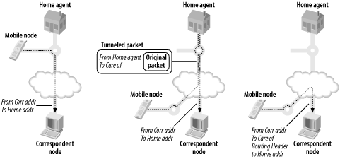
In order to support this, another router is placed on this home network. Its job is to maintain a list of all known mobile nodes; it’s called a Home Agent. The mobile nodes, when they move out of home network, register their changing addresses with the Home Agent. The address that a mobile node gets when it is on a different (“foreign”) link is called a care-of address. The mobile node establishes a binding between the care-of address and the home address by communicating with the Home Agent.
This is fine for correspondent nodes who want to send packets to the mobile host, but what about for communication in the other direction? The mobile node can’t just send packets with its home address, as these are likely to be blocked by ingress or egress filtering. Tunnelling back to the home agent might be possible, but could introduce significant latency or be prevented by firewalls. Thus, the approach taken is to send the packet from the care-of address, with a Destination option header saying what the source address should have been. This Destination header option is called the Home Address option.
Consequently, this means that the correspondent nodes must understand the Home Address option, and if they receive a packet with the home address option, the source address of that packet must be replaced with the home address when it is processed. A correspondent node can also support the same sort of binding between home-address and care-of address that Home Agents support, which allows them to send replies directly to the mobile node, without the intermediate step of sending them to the Home Agent.
So, the steps for sending a packet when mobile IP is in operation are:
Am I a mobile node replying to another node? If so, create reply packet with care-of address as the source address and add home address options header.
Am I a node replying to a mobile node and is its current care-of address in my binding cache? If so, create reply packet to care-of address as destination and add in home address as a part of routing extensions header.
Figure 3-6 shows the path that packets take from a mobile node to a correspondent node in various situations. Note that the packets always take a direct route. Figure 3-7 shows the path going in the opposite direction. Keep in mind that it is possible for the correspondent node to also be mobile. Before a mobile node uses any of these route optimizations, it will perform tests to ensure that they work correctly from the foreign network it is connected to.

In addition Mobile IPv6 defines additional ICMPv6 messages and options for home agent discovery and Destination options for maintenance of home address and care-of address binding. Like Router Renumbering, Mobile IPv6 also has serious security implications and must be used in combination with IPsec. Mobile IPv6 is described in considerable detail in RFC 3775.
Surprisingly, mobile phone networks do not plan to use Mobile IP at least in their first incarnations. This is because GPRS and 3G networks behave like a gigantic seamless layer 2 network. That is, there are no intermediate layer 3 nodes; every node is connected via tunnels back to the main router, the GGSN. Thus, there’s no real need for Mobile IP in this scenario.
At the time of writing IPv6 stacks have various degrees of support for Mobile IPv6. Support is not generally very complete, especially in release versions of software, though many vendors are monitoring the standard closely as has been finalized. For this reason we won’t say much about mobile IPv6 in the rest of this book, as it is just a little early to deploy on the platforms we consider. However, for those of you who are interested in playing around, various stacks are available; in particular, Microsoft have one available, but you currently have to sign an NDA to gain access to it. Contact Microsoft at [email protected] or through your usual support channel. Similarly Cisco mobile IPv6 is currently available as a technology preview; contact your Cisco representative for details.
Routing
Routing protocols are clearly very important to the operation of the Internet, but in a sense they are a separate issue from the problems of how low-level IP should operate.
So, how has IPv6 changed routing protocols? Well, the most obvious change you need to make is to allow IPv6 prefixes to be included, rather than IPv4 addresses. In fact, this is generally the only significant change between the IPv4 and IPv6 versions of well-known routing protocols.
Perhaps the most interesting changes in routing caused by IPv6
are in routing policy—in other words, not
affecting the prefix processing per se, but affecting the
administrative acquisition and control of prefixes. The routes that
can be advertised into the IPv6 Internet’s global routing table are to
be much more strictly controlled than in IPv4. For example, it is
hoped that people will not advertise individual /48 prefixes, because (remember!) these
should be aggregated into a bigger block advertised by their ISP.
We’ll talk more about the impact of this in Chapter 4.
For now, let’s have a quick look at the routing protocols you’re likely to encounter. First we’ll deal with IGPs (Interior Gateway Protocols). An IGP is used to route within an organization. IGPs include protocols such as RIP, OSPF, and IS-IS. After IGPs we’ll take a look at BGP, which is the main Exterior Gateway Protocol currently in use on the IPv6 Internet.
RIPng
RIPng is defined in RFC 2080 and is very similar to its IPv4 forebear. It is designed for use in small to medium organizations that don’t have a complicated routing setup. How does it work?
Well, each router sends messages (in UDP packets, port 521) that tell its neighbors what prefixes it knows how to reach and the metric associated with each prefix. A router may see a prefix advertised with several different metrics, so to choose the best one it adds a link related cost to each and then chooses the smallest. The cost assigned to each link is usually 1, so that the metric is actually a count of the number of links you must cross to reach that prefix.
Once a router has calculated the best available prefix and metric, it then advertises these new metrics and on to its neighbors. It also advertises prefixes that it can reach directly.
To stop routes hanging around forever, RIP expires routes that it hasn’t seen advertised recently and also considers a metric of 16 to be so big that the route isn’t worth considering.
Furthermore, it includes mechanisms for reducing the chance of routing loops, to only advertise changes and to avoid flooding the network in the case of frequent updates.
So, other than allowing IPv6 addresses in the protocol, what
are the IPv6 specific details in RIPng? Well, RIPng uses the
link-scope multicast address FF02::9 when it wants to send a message to
all its neighbors. Also, routers are expected to specify their
addresses as link-local addresses in RIP packets. Link-local
addresses are good (in this case) for routing because you know they
won’t change if the network is renumbered.
OSPF
With RIP, all you learn about a prefix is its metric, which tells you how many hops away it is. For this reason RIP is sometimes called a distance vector protocol. Sometimes the distance to a prefix isn’t enough to make a good routing decision.
OSPF has a different take on the problem. Rather than transmitting a prefix and a metric, each router transmits the information about the links attached to it, making it a link state protocol. This information is propagated through the network (in other words, routers pass this information on) and means that all routers have a full picture of the network. Then each router can make a decision based on the global situation about what routes it should use. The rule used is to choose the shortest path, where shortest is defined in terms of a combination of weights associated with each link.
Since OSPF routers have a full picture of the network, they don’t have the same problems with loops or maximum hop counts that RIP has. However, there is a significant amount of complexity required to make OSPF practical and stable, and much of the OSPF protocol deals with this. To understand the details of OSPF takes more space than we have here, and for more details we refer you to John Moy’s books on the protocol: OSPF: Anatomy of an Internet Routing Protocol and OSPF Complete Implementation (both published by Addison-Wesley).
OSPF for IPv6 is defined in RFC 2740, and it basically operates like a fully-featured IPv4 OSPF that understands IPv6 addresses instead of IPv4 addresses. Section 2 of the RFC is dedicated to describing the differences between OSPFv2 (RFC 2328) and and OSPF for IPv6. Perhaps the most interesting of these from an operational point of view are:
IPv6 interfaces typically have several addresses belonging to different IPv6 subnets. OSPF used to work on a per-subnet basis, but to fit in better with the idea of multiple subnets per link, it now works on a per-link basis.
Router IDs remain 32 bits wide and are written like IPv4 addresses. As your router may not actually have an IPv4 address, these can be assigned independently of IPv4 addressing. Router IDs are now always used to identify neighbors, rather than using IP addresses.
Like RIP, OSPF uses link-local addresses for the next routing hop. The
FF02::5andFF02::6multicast addresses are also used. Unlike RIP, OSPF isn’t run over TCP or UDP, but is a protocol of its own (using a Next Header value of 89).Authentication, if required, must now be done with IPsec. This means no more md5.
Integrated IS-IS
IS-IS is a routing protocol very similar in idea to OSPF: it is also a link-state protocol and uses shortest-path routing, again based on metrics assigned to links. The main difference between IS-IS and OSPF is that IS-IS is part of the OSI protocol suite and turns out to be slightly more protocol agnostic than OSPF. The original additions to IS-IS for routing IPv4 are described in RFC 1195 and the minor extras for IPv6 are now being finalized at the IETF.
IS-IS, when used to route IP, is sometimes referred to as integrated IS-IS. Here “integrated” refers to the fact that you could run a single IS-IS instance on a router to route IP and ISO protocols. The advantages of this include reduced processing overhead on routers, and also a single routing protocol for network management staff to worry about.
With the appearance of IPv6, a single IS-IS instance can now route IPv4, IPv6 and ISO protocols. This has appeal for some network operators, and they have moved to IS-IS so that they can route their IPv4 and IPv6 traffic with a single protocol. Others have chosen IS-IS just for IPv6, so that they have a degree of protocol redundancy within their network (or maybe just to get a feel for a different IGP). Possibly for these reasons, it seems that IS-IS may end up being the most popular IGP for IPv6.
Interestingly, from a protocol point of view, IS-IS doesn’t use TCP, UDP, IPv4 or IPv6, but instead uses its own ISO protocol for the exchange of routing information. This means that configuring IS-IS involves assigning ISO addresses to the routers in your network that will speak IS-IS.
BGP-4+
The BGP protocol is different from the previous routing protocols we’ve discussed for a few reasons. First, it is designed for routing between many independent networks, rather than routing within an organization. It is the protocol that determines the routes between all the networks in the Internet. To make things manageable, each network is treated as a black box: BGP can see where the networks connect to each other, but it can’t see inside the networks. These black boxes are called autonomous systems (ASs).
Even still, the number of networks that BGP has to deal with is large and the number of links even larger. For this reason, using a link-state protocol isn’t feasible. A distance-vector protocol isn’t practical either because there are just too many hops and loops in the Internet.
BGP operates in a hybrid area between distance-vector and link-state. As in distance-vector, a router only tells its neighbors about the best route it has to a network, but rather than just telling them the metric of this route, it also communicates other information, including the list of ASs the best route goes through. This means that BGP may not know the state of all the links in the Internet, but it does at least know the hops along the routes it wants to use. This information can be used to avoid routing loops by discarding routes that would go through an AS twice.
As well as this AS path information, a BGP router also communicates a selection of information about how desirable various routes are. There are a dizzying array of rules and configuration knobs that can be used to get BGP to route traffic in particular ways. A lot of the operational complexity of BGP arises from these parameters.
In terms of low-level details, BGP-4 (RFC 1771) has a set of extensions to deal routing information for arbitrary protocols (RFC 2858). The details for IPv6 are made explicit in RFC 2545.
BGP actually runs over TCP (port 179), which means it can use IPv4 or IPv6 for transport. However, the address of the remote router can be important for calculating next hops, so if you are transporting IPv6 routing information over an IPv4 TCP session you may need to explicitly configure information about the next hop. (Typically, one would bring up two BGP sessions in parallel—one over IPv4, one over IPv6—and over each session one would exchange only the routing information specific to that protocol.)
Like OSPF, BGP also uses a router ID in the protocol, which remains a 32-bit number. For routers with IPv4 addresses, this ID is usually one of those addresses. If you have an IPv6-only router, the Router ID has to be configured manually.
BGP does have limitations that may become a problem as time progresses. For example, ASs are identified by 16 bit numbers, so some day we’ll run out of AS numbers, just like IPv4 addresses. A protocol called IDRPv2 was supposed to address these, and other more complex issues. Today, however, BGP remains the routing protocol of the IPv6 backbone.
Security
IPv6 enhances network security considerably. Probably the most important contribution it makes is not a technical contribution, but rather a matter of policy—the standard mandates that an IPv6 stack must not be implemented without supporting some form of encryption. It’s important to note that this encryption is not at an application layer; that is, it’s not a separate ad-hoc mechanism which is differently configured in mail programs than in web browsers than in video streaming applets—it is at a lower layer and can also secure things like neighbor discovery.
This was quite an achievement by the IETF. There are certainly very many jurisdictions in the world that use computers; many of them have severe anti-encryption laws; some of them prohibit its use entirely.
The form of security, IPsec, is already familiar to many as it is the basis of many VPN (virtual private network) systems that are already deployed. IPsec is quite a complicated architecture; see RFC 2401 for more details. In IPv6 it is implemented using extension headers that say that the remainder of the packer is encrypted (the ESP header of RFC 2406) or cryptographically signed (the AH header of RFC 2402). These are basically the same techniques as used in IPv4.
IPsec does, however, come with some downsides. For example, if traffic is regularly encrypted within your network, then debugging or security-related packet-content sniffing is impossible, unless you have the key. For that reason alone, some network administrators insist on configuring a static key for intra-site communication between machines, for ease of debugging. There have been efforts made, however, to ensure that header encryption (as opposed to content encryption) is not mandatory under all circumstances.
Quality of Service
Quality of service, henceforth referred to as QoS, is a complicated area. The core concept is quite simple: we, both as network administrators and as users, want to ensure that a certain application can have guaranteed performance on a certain network. When desired by a user, this often translates to statements such as “I wish I could download that ISO before I’ve got to catch my bus...” and, when desired by a network administrator, generally translates as “How can I stop those ISO downloaders killing the rest of the network?”
Generally, the kind of application we want to guarantee performance for is a multimedia application, not the standard HTTP or SMTP transactions that take place billions of times a day (although in some cases we may want to guarantee that a certain portion of the network will be set aside for critical services). This is because multimedia applications are amongst the most sensitive to packet loss and jitter, given the necessity to have data arrive at the right time for reassembly and display. There are various theories regarding how this should be done:
Smart network, stupid end hosts
Stupid network, smart end hosts
Overdimensioning
The first two schemes differ over where to place the intelligence involved in making QoS decisions, while the last attempts to avoid the problem entirely. Exactly what scheme will provide the best QoS under all circumstances is unclear. Different schemes require different facilities to be available. Rather than make a call on how QoS should work, IPv6 provides some generic facilities that should help QoS designers. These include some fields in the IPv6 header and, of course, extension headers.
There are two ways in which the IPv6 header provides for manipulable QoS. One is the traffic class field, the other is the 20 bit flow label in the IPv6 header. Note, that these fields are available in the base IPv6 header, and so are immediately available to routers, regardless of the Extension Headers that may follow.
The traffic class field is discussed in RFC 2460, but leaves the classes to be defined after future research. Differentiated Services, one of the existing mechanisms used to provide QoS, provides its interpretation of the traffic class field in RFC 2474. In a network providing QoS via DiffServ routers would decide to give packets preferential treatment based on RFC 2474’s interpretation of the traffic class field.
To explain what a flow label is, we must say what a flow is. A flow is some specified subset of the traffic making its way from one part of a network to another. Usually the flow is defined in terms of all the traffic from a particular running application, host or network to another.
In IPv6, a flow is envisaged as a one way association between an application on one host and another application, usually elsewhere in the network. A packet is identified as belonging to a particular flow by its source and destination IPv6 addresses and the flow label. The only special value for the flow label is zero, which indicates that the packet doesn’t belong to any flow in particular.
The flow label mechanism makes flows easily identifiable, so an application or the OS can request particular handling of packets within a flow by the intervening routers and the end host(s).[20] The request for special treatment could be made using a protocol like RSVP. The idea of RSVP is that a message can be sent to the routers a flow passes through describing the special treatment that the flow requires.
Flow labels will usually be selected randomly to allow for efficient usage of hash tables, though routers aren’t supposed to depend on this. There are even proposals to allow routers to rewrite flow labels to allow their use for MPLS-like routing. The description of the flow label’s usage is described in RFC 3697.
Because of the general flexibility of IPv6, there are also other ways that QoS could be provided for, say by using the Routing header or Hop-by-hop options header. However, all these techniques are still areas of active research and deployment is still limited to relatively special situations. Whatever QoS system prevails, IPv6 should have the features to support it.
Today, in the real world™, the most common and perhaps the simplest approach has been to overdimension. In other words, making the capacity of links substantially more than your total projected traffic volume, so that you never experience the congestion and network performance deterioration that QoS is supposed to help you manage. It may not be cheap, but it does tend to work. Unfortunately if there are any low capacity links in your organization at all, chances are someone will want to do something exotic with them sooner or later.
The Promise of IPv6
Let’s finish off this chapter with a quick review of what the features offered by the design of IPv6 are.
Simplicity and Flexibility
IPv6’s scalability, the darling of many press releases, is perhaps best broken into two capabilities. First, the capability of the protocol to rise to the task of addressing and routing both the existing and the future Internet. We think everyone can agree that IPv6 has been engineered with this in mind, by allowing lots of address space for hosts and countering the routing problems with a more hierarchical address space, while being flexible enough for future developments. Second, the ability of the protocol to be extended naturally to meet future, as yet unknown, requirements. A very important component of this is the Extension Headers facility.
Mobility and Security
IPv6 offers significant mobility and security features which, unfortunately, by their nature, are not as simple as might be desired. While support for IPsec is widely available, configuring for interoperability can be tricky. Mobility is at an earlier stage of development, and while implementations are available, full implementations are not yet widely shipped.
[2] There are large numbers of hosts hidden behind NAT and it does not account for hosts without DNS records, of which there are a sizable number.
[3] With DHCPv6 it is possible for a client to request non-address-related configuration information (such as DNS resolvers) while obtaining their addresses via the autoconfiguration of interface IDs.
[4] See RFC 3177 for further details.
[5] As Bill Gates is alleged to have said, `’640k should be enough for anybody.”
[6] We’ll talk about the RIRs and their address allocation policies in Section 4.2.5 of Chapter 4.
[7] Of course, the link may involve tunnelled or encapsulated traffic, using MPLS or some other mechanism, but these operate in the layers below IPv6.
[8] Note well that IPv6 NetBIOS is not possible with Windows—which means your hostname resolution may well have to be done by Active Directory, Dynamic DNS or IPv6’s node information queries. Complications in naming and addressing mean that link-local addressing alone is a bad idea for more complex networks.
[9] Like a business campus or university, not a web site!
[10] A well-known multicast address is one for some well-known service, like “all DHCPv6 servers.” A transient address is one that is created dynamically, for example to send a specific audio stream to a group of users.
[11] Solicited node multicast addresses are explained in Section 3.3.4.1 earlier in this chapter.
[12] The security implications of this are not unlike the security implications of duplicate addresses in IPv4 networks, with the key difference being that machines won’t “fight it out” between themselves for the address.
[13] Large being defined as having enough routers to make it worthwhile doing automatically.
[14] The hierarchical routing model stems from the policy of only assigning provider aggregate addressing in IPv6. The IPv4 address space is assigned discontiguously, and machines that are close within a network often have radically different IPv4 addresses.
[15] As an example, the MTU on Myrinet is, in theory, unlimited. In practice, you’d probably want to think twice about making the MTU unusually large.
[16] This used to be a security hot button in IPv4, when authentication based on source IPv4 address was common and packet filtering was not.
[17] The smallest IPv4 header is 20 bytes, compared to a fixed size of 40 bytes for IPv6.
[18] In fact this is only one of many ways of doing it. The complexity comes in attempting to compensate for protocols that do not retransmit in the case of error.
[19] RFC 3242 reports they can get these headers down to one (!) octet in certain circumstances.
[20] Yep—the destination address can be a multicast address.