Chapter 4: Creating Animations
Animations and interactive visualizations can tell stories that static plots cannot. Also, both are more engaging for the final audience. As shown in the previous chapter, interactive visualization can let us interact with a variable to visualize its impact, among other things. Instead, animations use the time dimension to encode that variable. The encoded variable can be time since animations are well suited to show how a process evolves through time. Another advantage of animations is that they are much easier to distribute than interactive visualizations.
In this chapter, we are going to learn how to create animations using Plots and Makie. We will also introduce Javis, a drawing library, which we will use to generate animations with Julia. Then, we will learn about the Animations package, which will help us move objects in our canvas. By the end of this chapter, you will know how to create and distribute simple animations using Plots, Makie, and Javis.
In this chapter, we're going to cover the following main topics:
- Easy animation using Plots
- Animating Makie plots
- Getting started with Javis
Technical requirements
For this chapter, you will need Julia, Pluto, and IJulia installed. You will also need a web browser with an internet connection. The Pluto and Jupyter notebooks for this chapter can be found in the Chapter04 folder of this book's GitHub repository: https://github.com/PacktPublishing/Interactive-Visualization-and-Plotting-with-Julia. You will also need to install the Plots package. This chapter also requires GLMakie, Animations, and Javis, but Pluto will automatically install them as required.
Easy animation using Plots
In this section, we will learn what animations are and how we can create them with Plots. We will also discuss the Animations package, which will help us interpolate between positions. We are also going to take advantage of Animations when working with Makie and Javis. But let's start with the most straightforward animation tool available in Julia: Plots.
Animations are simply a succession of slightly similar images in time that give the sensation of movement. Each of those images is a frame of the animation. The Plots package does precisely that; it provides an Animation object that you can add one frame at a time to. Each frame is a static PNG image that's created using Plots. It's up to us to generate each frame with the slight change that's needed to create a pleasant animation.
We can save animations in different formats. The Plots package offers the following format options:
- gif: GIF is the most popular and widespread file format for small animations. Almost all platforms, including old web browsers, support this format. You can even use it on social media platforms. GIF is also the only animation format that the Julia extension for Visual Studio Code (VS Code) can display out of the box. GIFs are usually low quality compared to the other options as they only support 256 colors and low frames per second (FPS). Because of its lossless compression, complex animations can lead to heavy files. Note that the first reproduction of a heavy GIF file could be slow.
- webm: Most modern web browsers support WebM. It offers higher quality and smaller file sizes than the previously mentioned GIF format.
- mp4: MP4 is one of the most popular formats; therefore, almost all platforms support it. It is also helpful for sharing videos on social media. It offers small file sizes while keeping good quality. However, WebM files tend to be a little smaller than MP4 files while maintaining similar quality.
- mov: The MOV format, also known as the QuickTime File Format (QTFF), is the least supported format in this list. It offers the highest quality, but it also generates the heaviest files.
For each of these formats, there is a function with the same name in lowercase. Those functions can take an Animation object and save it in that format. There is also a @gif macro, which can help you create a GIF animation quickly. When displayed using HTML, for example, inside Pluto or Jupyter notebooks, the MOV, MP4, and WebM formats offer a series of buttons to control video reproduction. However, support would depend on your operating system, web browser version, and available plugins. Note that you can also reproduce those animation files using movie players. In particular, the VLC media player supports all those formats while being free, cross-platform, and open source.
Let's explore this by creating a simple animation using Plots. In this example, we are going to move a point around the origin while following the unit circle. First, we will show you the most verbose approach to help you gain an idea of what Plots is doing. Later, we will learn how to do this more easily:
- Open the Julia REPL and execute using IJulia; notebook() to open Jupyter.
- Create a new Jupyter notebook.
- Execute using Plots in the first cell to load the Plots package and the default GR backend; we do not need any other packages to create a Plots animation.
- Execute the following code in a new cell:
function plot_frame(angle)
scatter(
[cos(angle)],
[sin(angle)],
ratio=:equal,
xlims=(-1.5, 1.5), ylims=(-1.5, 1.5),
legend=:none)
end
Here, we have created the function that we will use to create each frame of the animation. For the animation, we will slightly change the value of the internal angle for each frame and display a point at the coordinates where the arc ends. In other words, we will create a scatter plot with a single point located at the x and y coordinates, as determined by the cosine and the sine of a given angle. So, we use a vector with a single element for the x and y coordinates. As shown in the examples in Chapter 3, Getting Interactive Plots with Julia, we have set the limits for the axes so that they fix our canvas; otherwise, we would see a fixed point and changing axes. We have also set the ratio to :equal to ensure that we have a well-proportionated circle, and we have set the legend to :none so that we have a cleaner canvas.
- Run the following code in an empty cell:
anim = Animation()
This creates an Animation object that, at the moment, has no frames. The Animation object contains the path to a temporal directory, where the frames will be stored. Great! Now, it is time to create the frames of our animation.
- Create a new cell and execute the following code:
for angle in 0:0.05:2pi:
plt = plot_frame(angle)
frame(anim, plt)
end
The preceding code iterates from 0 to 2 times pi to get the value of the angle variable using small steps of 0.05. Therefore, we are creating the slight change we need between frames. For each iteration, we create the plot object containing the image for a frame. Then, we store the current frame in the animation using the frame function.
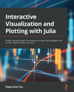
- Execute anim in a new cell to see the Animation object. The frame field should now contain a vector of PNG images.
- In an empty cell, execute gif(anim). This function will tell you the address of the temporal file containing the animation, and it will show the animated GIF inline in the notebook. The following screenshot shows what you will see after executing these last two steps; note that one of the frames of the animation has been frozen here:
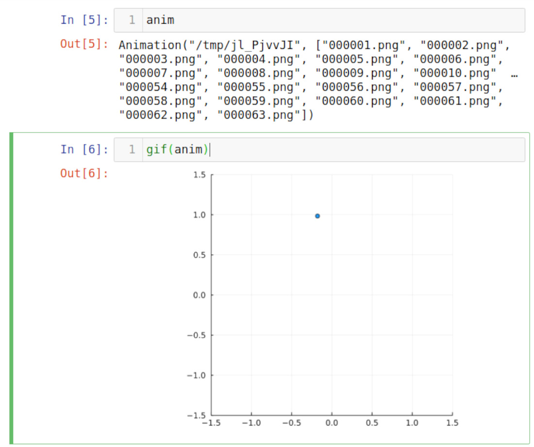
Figure 4.1 – Animated GIF inline on our Jupyter notebook
Perfect! You have created your first animation with the Plots package. Note that the gif function, similar to the mov, webm, and mp4 functions, can take a second position argument to specify the filename of the final animation. You must choose the extension based on the format; therefore, it should be equal to the function's name. These functions can also take the following keyword arguments:
- fps: This keyword argument determines the frame rate as the number of FPS; it defaults to 20.
- loop: This keyword argument takes an integer number indicating the number of times the player should reproduce the animation. The GIF format supports it well. The default value is 0, meaning to loop it infinitely. You can set this value to -1 to avoid looping the animation. If you set this to n, with n greater than 0, the player will play the animation n + 1 times.
For example, gif(anim, "first_animation.gif", fps=50, loop=-1) will save the GIF as first_animation.gif, so the animation will be faster than the default one, and it will not loop.
We have created an animation in the most verbose way we can by explicitly populating an Animation object. We did this in Jupyter as doing the same in Pluto won't play nicely with reactivity. That's because the frame function modifies the Animation object in a way Pluto cannot figure out. So, the same example in Pluto should create the Animation object and call the frame function in the same cell by using a single code block that's been defined, thanks to the begin and end keywords. Thankfully, Plots offers a more convenient way to create animations that work nicely on all the editors – the @animate macro. Let's make a more straightforward version of our animation by using it:
- Open a new Pluto notebook.
- Execute using Plots in the first cell.
- Create a new cell and execute the following code block:
function plot_frame(angle):
scatter(
[cos(angle)],
[sin(angle)],
ratio=:equal,
xlims=(-1.5, 1.5), ylims=(-1.5, 1.5),
legend=:none)
end
As we did previously, we have created a function that creates the image we want for each frame. We have done this to keep our code clean, but creating a dedicated function is not mandatory since you can create any plot inside the for loop.
- Execute the following code in a new cell:
anim = @animate for angle in 0:0.05:2pi
plot_frame(angle)
end
As you can see, we have created and populated the Animation object using the @animate macro in front of the for loop that renders each frame. We do not need to call the frame function now since the @animate macro automatically does this.
- Create a new cell and execute gif(anim) to view our animation.
As you can see, everything has been more straightforward in this example. The @animate macro is the preferred way to create animations with Plots. It can also take some extra flags after the for loop block that could be helpful when you're creating animations:
- every: The every flag takes an integer, n, to save a frame every n iterations.
- when: The when flag takes a Boolean expression that will save a frame each time the expression is true.
For example, the following code uses the @animate macro and its every flag to create a faster but less smooth animation by taking fewer frames:
anim_fast = @animate for angle in 0:0.05:2pi
plot_frame(angle)
end every 10
gif(anim_fast)
The following code uses the when flag of @animate to save frames, but only when angle is between 0 and pi:
anim_partial = @animate for angle in 0:0.05:2pi
plot_frame(angle)
end when 0 <= angle <= pi
gif(anim_partial)
In these examples, we created an Animation object and then called the gif function to render it. This gave us a lot of freedom to choose how to render it as we can select the file format, the frame rate, and the looping behavior. However, this can be cumbersome for throwaway animations we want to see quickly. For those cases, Plots exports the @gif macro, which works like the @animate macro, but it returns a GIF file rather than an animation object.
Now, you know how to create animations with Plots and save them in different formats for distribution. We have created a simple animation, but you can animate more complex figures by taking advantage of all the available Plots features. In the next section, we will explore the Animations package, combined with Plots, to move objects around our canvas.
Using the Animations package
The Animations package helps us create animations by interpolating between different positions in time. You can control the interpolation of the relevant values using easing functions. These easing functions will determine the speed and acceleration of the movement in the animation. For example, the noease easing function will avoid any interpolation; all the animation frames will show the object at the initial position, except for the last one. The stepease function is similar, but it will let us choose when the position changes. The linear easing function will gradually change the object positions between frames without acceleration. For example, we can make a point rotate around the origin at the same speed, as in our previous animation, using the linear easing function to interpolate the angle values. Any other easing function will create an accelerated movement. Let's look at an example by using the Animations package and the polyio easing function to make our point go faster for angle values around pi:
- Open a new Pluto notebook.
- Execute using Plots, Animations in the first cell to load the libraries.
- Create a new cell and execute the following code:
angle_animation = Animations.Animation(
0, 0.0,
polyio(3),
1, 2pi
)
This creates an Animation object from the Animations package. We needed the Animations.Animation qualified name as Plots and Animations both export an Animation type. We created an animation that interpolates the angle value from 0.0 at time 0 to 2pi at time 1. We set that in the Animation constructor by passing the number pairs 0, 0.0 and 1, 2pi. Each pair creates a Keyframe object, where the first number determines the time and the second is the value to interpolate. This last value should be a floating-point number. If we explore the output of that cell, we will see that the frame field of the Animation object has a vector of Keyframe objects. We indicated the easing functions between the pair of numbers that are determining the keyframes. In this case, we used a polyio, which creates a polynomial easing. This function takes one parameter to indicate the power of the polynomial function, but not all the easing functions take parameters.
- Execute times = 0:0.005:1 in a new cell; this creates our time variable. The range should include the time values of our keyframes.
- In a new cell, execute the following code:
plot(times, angle_animation.(times),
xlab="t", ylab="angle", legend=false)
In this way, we can visualize how the value of the angle changes as a function of our time variable. Here, we have used dot broadcasting to calculate the angle value for each time point. This is possible because the Animation object, when called as a function using a Real number, will return the value at that time point. The following screenshot shows the plot with the shape that was created by the polyio easing function. The function's slope indicates that the fastest speed will be at time 0.5:
Figure 4.2 – A change in the angle value through time
- Create a new cell and execute the following code:
anim = @animate for time in times
angle = at(angle_animation, time)
scatter([cos(angle)], [sin(angle)],
xlims=(-1.5, 1.5), ylims=(-1.5, 1.5),
ratio=:equal, legend=:none)
end
This code creates a Plots Animation object using the @animate macro. Inside the for loop, there's a call to scatter, which is the same as in the previous examples. The main difference is that we defined the angle value using the at function, which takes the interpolated value at a given time. In fact, at(angle_animation, time) is equivalent to angle_animation(time).
- Execute gif(anim) in a new cell to see the animation inline in the notebook.
We now have a rotating point with varying speeds! We determined the speed change using the polyio function. Animations also exports other easing functions, such as polyin and polyout. Some easing functions, such as polyio, can take keyword arguments. For example, you can use the yoyo easing function and its n argument to create a back-and-forth movement and determine the number of repetitions.
Now that we've learned how to create animations using Plots and learned how to use the Animations package to help us create complex movements, let's learn how to create animations using Makie.
Animating Makie plots
There are many ways to animate Makie plots; here, we will explore one of them. The general idea is similar to the one presented for Plots; we need to modify a plot to create the animation frames iteratively. To achieve that, Makie offers the record function, which can use Figure, FigureAxisPlot, or Scene to animate an iterator that returns the values changing through time and a function that uses these values to modify the plot. This function is the first argument to record, so we can use the do syntax to create it. Inside that function, you can rely on the Observables mechanism, which we discussed in Chapter 3, Getting Interactive Plots with Julia. The advantage of this is that Makie updates only parts of the plot that have changed in each frame, rather than rendering an entirely new figure, which is what Plots does. Let's explore this by creating a GIF animation of the rotating point using GLMakie and Pluto:
- Create a new Pluto notebook.
- Execute using GLMakie in the first cell to load Makie and its OpenGL-powered backend.
- Create a new cell and execute angle = Observable(0.0)
- In a new cell, run the following code:
point = @lift Point2(cos($angle), sin($angle))
Here, we have used the @lift macro to generate a point observable that Julia will update each time the value of the angle observable changes.
- Run the following code in a new cell:
plt = scatter(point,
axis=(aspect=DataAspect(),
limits=(-1.5, 1.5, -1.5, 1.5)))
The preceding code creates a scatter plot showing the point observable. We set the correct aspect to see the circular trajectory and the proper limits to ensure that the axis doesn't change through the animation. You will see the scatter plot inline in the notebook.
- Add a new cell after that one and execute the following code:
anim = record(plt, "rotating.gif", 0:0.05:2pi) do value
angle[] = value
end
The preceding code will create the animation by creating a frame for each value on the 0:0.05:2pi iterator. The record function will pass each iteration value to the anonymous function we created with the do syntax. In this case, the anonymous function is only updating the value of the observable angle. This update causes Makie to change the necessary elements of the existing plot. You will see that Makie shows the changes in a GLFW window. The record function returns the path to the animation file. We have determined the name of that file in the call to the record function. The filename extension will select the output format; in this case, we are creating a GIF file. Let's use LocalResource from PlutoUI to inline the animation file in our notebook.
- Create a new cell and execute using PlutoUI.
- Execute LocalResource(anim) in a new cell to see the animation.
With that, we have created our first animation using Makie by taking advantage of the same system we learned how to use to create interactive plots. Here, we saved our animation in GIF format, as indicated by the gif extension. You can also store animation files using the previously mentioned extensions and formats; that is, webm and mp4. Makie cannot save animations in MOV format, but contrary to Plots, it also offers the Matroska Multimedia Container (MKV) format. This format is generated by default when you use Makie.
Now that we know how to create animations using Makie, let's learn how to use the Javis package for the same purpose.
Getting started with Javis
Javis is different from the previously mentioned options as it is not a plotting library like Plots or Makie. Javis only focuses on creating animations. It uses and re-exports objects from Luxor, a 2D drawing package based in Cairo. Here, we will quickly introduce the package by animating our rotation point. However, be aware that you can do much more with it. Let's learn how to create our animation with Pluto:
- Create a new Pluto notebook and execute using Javis in the first cell.
- Add a new cell and run the following code:
function ground(args...)
background("white")
sethue("blue")
end
The preceding code creates a function that will take the Video object, the object to animate, and the current frame. Javis will give those inputs to all user-defined functions, so it is common to use args... for their arguments. This function calls background to set the background color and sethue to select the default color for our objects.
- In a new cell, execute the following code:
function create_point(args...)
circle(O, 10, :fill)
end
This function will create the object to animate. In this case, we will create a circle with a radius of 10 at the origin. Javis defines O as an alias for Point(0.0, 0.0).
- Run the following code in a new cell:
begin
video = Video(500, 500)
Background(1:50, ground)
point = Object(create_point, Point(100, 0))
act!(point,
Action(anim_rotate_around(2pi, 0.0, O)))
end
Here, we have created a Video object for our animation. Javis's functions and objects will modify the previously created video. Therefore, we need to execute them in the same Pluto cell, as Pluto cannot keep track of those changes. For example, here, we have set Background for our Video using the previously defined function. We have also determined that our video will have 50 frames using the 1:50 range. Then, we created a point object using the previously defined function and placed it at Point(100, 0). Note that Point(0.0, 0.0) is the center of the canvas. Finally, we used the act! function to assign an Action to our object. In this case, we make our point rotate around the origin from angle 2pi to 0.0.
- Create a new cell and execute render(video; pathname="javis_animation.gif") to save the animation. The file extension determines the file format; the available options are gif and mp4. You will see the animation inline in the Pluto notebook.
Great! We have created our first animation with Javis.
Summary
In this chapter, we learned how to create animations using Plots, Makie, and Javis. We have also learned how to use the Animations package to make complex movements with a few lines of code. While we have learned how to use the Animations package with Plots, you can also take advantage of it with Makie and Javis. Now, we can choose the correct format to distribute our animations in. You will find this new knowledge incredibly helpful while creating and sharing compelling animations. This, in turn, will help you visualize data that changes through time, make didactic animated figures, and draw attention to your plots.
In the next chapter, we will learn about the different adaptations of the grammar of graphics available in Julia.
Further reading
If you want to learn more about creating animations with Julia, please read the documentation for the packages we used in this chapter:
- Documentation for Plots: http://docs.juliaplots.org/latest/animations/.
- Documentation for Makie: https://makie.juliaplots.org/stable/documentation/animation.
- Documentation for the Animations package: https://jkrumbiegel.com/Animations.jl/stable/.
- In this chapter, we have only scratched the surface of what Javis can offer; you can explore it more by following the tutorials here: https://wikunia.github.io/Javis.jl/stable/.