Chapter 8

Introduction to the digital VTR

8.1 History of DVTRs

The first production DVTR, launched in 1987, used the D-1 format which recorded colour difference data according to CCIR-601 on ¾-inch tape. D-1 was too early to take advantage of high-coercivity tapes and its recording density was quite low, leading to large cassettes and high running costs. As a result, D-1 found application only in high-end post-production suites. The D-2 format came next, but this was a composite digital format, handling conventional PAL and NTSC signals in digital form, and derived from a format developed by Ampex for an automated cart. machine. The choice of composite recording was intended to allow broadcasters directly to replace analog recorders with a digital machine. D-2 retained the cassette shell of D-1 but employed higher-coercivity tape and azimuth recording (see Chapter 6) to improve recording density and playing time. Early D-2 machines had no flying erase heads, and difficulties arose with audio edits. D-3 was designed by NHK, and put into production by Panasonic. This had twice the recording density of D-2; three times that of D-1. This permitted the use of ③-inch tape, making a digital camcorder a possibility. D-3 used the same sampling structure as D-2 for its composite recordings. Coming later, D-3 had learned from earlier formats and had a more powerful error-correction strategy than earlier formats, particularly in the audio recording.

By this time the economics of VLSI chips had made compression in VTRs viable, and the first application was the Ampex DCT format which used approximately 2:1 compression so that component video could be recorded on an updated version of the ¾-inch cassettes and transports designed for D-2. When Sony were developing the Digital Betacam format, compatibility with the existing analog Betacam format was a priority. Digital Betacam uses the same cassette shells as the analog format, and certain models of the digital recorder can play existing analog tapes. Sony also adopted compression, but this was in order to allow the construction of a digital component VTR which offered sufficient playing time within the existing cassette dimensions.

The DV format was designed as a consumer digital device and the very small cassette allows highly miniaturized products. In the DV format relatively heavy compression is used to obtain a bit rate of 25 Mbits/s on tape. The results obtained from DV were so remarkable that professional equipment was developed from it under the name of DVCPRO. DVCPRO subsequently introduced higher bit rates of 50 and 100Mbits/s.

The D-5 component format is backward compatible with D-3. The same cassettes are used and D-5 machines can play D-3 tapes. However, the tape speed is doubled in the component format in order to increase the bit rate to 360Mbits/s. D-5 recorders have become very useful in the development of HDTV because with mild compression they can easily record HDTV formats. Some D-5 machines have also been made which can run at 700Mbits/s.

The D-6 format is intended for high bit rate use in HDTV applications and uses a large number of heads in parallel. D-9 uses the compression algorithms of DVC to create a production-grade DVTR format using VHS-sized cassettes at lower cost than earlier formats.

The popularity of the DVTR has been eroded by the enormous growth of disk-based production equipment, but for archiving purposes and in portable applications the tape medium still offers advantages and will not go away readily. In the future recording technology will continue to advance and further tape formats will emerge with higher performance. These will be needed to support the emerging high-definition and electronic cinema applications.

8.2 The rotary-head tape transport

The high bit rate of digital video could be accommodated by a conventional tape deck having many parallel tracks, but each would need its own read/write electronics and the cost would be high. However, the main problem with such an approach is that the data rate is proportional to the tape speed. The provision of stunt modes such as still frame or picture in shuttle are difficult or impossible. The rotary-head recorder has the advantage that the spinning heads create a high head-to-tape speed offering a high bit rate recording with a small number of heads and without high linear tape speed. The head-to-tape speed is dominated by the rotational speed, and the linear tape speed can vary enormously without changing the frequencies produced by the head by very much. Whilst mechanically complex, the rotary-head transport has been raised to a high degree of refinement and offers the highest recording density and thus lowest cost per bit of all digital recorders.

Figure 8.1 shows that the tape is led around a rotating drum in a helix such that the entrance and exit heights are different. As a result, the rotating heads cross the tape at an angle and record a series of slanting tracks. The rotating heads turn at a speed which is locked to the video field rate so that a whole number of tracks results in each input field. Time compression can be used so that the switch from one track to the next falls within a gap between data blocks. Clearly, the slant tracks can only be played back properly if linear tape motion is controlled in some way. This is the job of the linear control track which carries a pulse corresponding to every slant track. The control track is played back in order to control the capstan. The breaking up of fields into several tracks is called ‘segmentation’ and it is used to keep the tracks reasonably short. The segments are invisibly reassembled in memory on replay to restore the original fields.

Figure 8.1 A rotary-head recorder. Medical scan records long diagonal tracks.

Figure 8.2 shows the important components of a rotary-head helical scan tape transport. There are four servo systems which must correctly interact to obtain all modes of operation: two reel servos, the drum servo and the capstan servo. The capstan and reel servos together move and tension the tape, and the drum servo moves the heads. For variable-speed operation a further servo system will be necessary to deflect the heads.

Figure 8.2 The four servos essential for proper operation of a helical-scan DVTR. Cassette-based units will also require loading and threading servos, and for variable speed a track-following servo will be necessary.

There are two approaches to capstan drive, those which use a pinch roller and those which do not. In a pinch roller drive, the tape is held against the capstan by pressure from a resilient roller which is normally pulled towards the capstan by a solenoid. The capstan only drives the tape over a narrow speed range, generally the range in which broadcastable pictures are required. Outside this range, the pinch roller retracts, the tape will be driven by reel motors alone, and the reel motors will need to change their operating mode; one bcomes a velocity servo whilst the other remains a tension servo.

In a pinch-rollerless transport, the tape is wrapped some way around a relatively large capstan, to give a good area of contact. The tape is always in contact with the capstan, irrespective of operating mode, and so the reel servos never need to change mode. A large capstan has to be used to give sufficient contact area, and to permit high shuttle speed without excessive motor rev/min. This means that at play speed it will be turning slowly, and must be accurately controlled and free from cogging. A multi-pole ironless rotor pancake-type brush motor is often used, or a sinusoidal drive brushless motor.

The simplest operating mode to consider is the first recording on a blank tape. In this mode, the capstan will rotate at constant speed, and drive the tape at the linear speed specified for the format. The drum must rotate at a precisely determined speed, so that the correct number of tracks per unit distance will be laid down on the tape. Since in a segmented recording each track will be a constant fraction of a television field, the drum speed must ultimately be determined by the incoming video signal to be recorded. To take the example of a 625-line Digital Betacam, having two record head pairs, six tracks or three segments will be necessary to record one field, and so the drum must make exactly one and a half complete revolutions in one field period, requiring it to run at 75 Hz. The phase of the drum rotation with respect to input video timing depends upon the time delay necessary to shuffle and interleave the video samples. This time will vary from a minimum of about one segment to more than a field depending on the format.

In order to obtain accurate tracking on replay, a phase comparison will be made between offtape control track pulses and pulses generated by the rotation of the drum. If the phase error between these is used to modify the capstan drive, the error can be eliminated, since the capstan drives the tape which produces the control track segment pulses. Eliminating this timing error results in the rotating heads following the tape tracks properly. Artificially delaying or advancing the reference pulses from the drum will result in a tracking adjustment.

8.3 Digital video cassettes

The D-1, D-2 and D-6 formats use the same mechanical parts and dimensions in their respective ¾-inch cassettes, even though the kind of tape and the track pattern are completely different. The Ampex DCT cassette is the same as a D-2 cassette. D-3 and D-5 use the same ③-inch cassette, and Digital Betacam uses a ③-inch cassette which is identical mechanically to the analog Betacam cassette, but uses different tape. The D-9 format uses a VHS cassette shell again with different tape.

The use of a cassette means that it is not as easy to provide a range of sizes as it is with open reels. Simply putting smaller reels in a cassette with the same hub spacing does not produce a significantly smaller cassette. The only solution is to specify different hub spacings for different sizes of cassette. This gives the best volumetric efficiency for storage, but it does mean that the transport must be able to reposition the reel drive motors if it is to play more than one size of cassette.

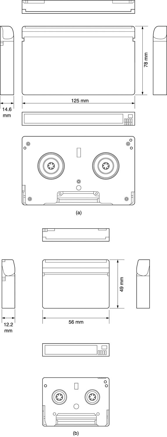
Digital Betacam offers two cassette sizes, whereas the other formats offer three. If the small, medium and large digital video cassettes are placed in a stack with their throats and tape guides in a vertical line, the centres of the hubs will be seen to fall on a pair of diagonal lines going outwards and backwards. This arrangement allows the reel motors to travel along a linear track in machines which accept more than one size. Figure 8.3 compares the sizes and capacities of the various digital cassettes.

Figure 8.3 Specifications of various digital tape formats compared.

8.4 DVTR block diagram

Figure 8.4(a) shows a representative block diagram of a full bit rate DVTR. Following the convertors will be the distribution of odd and even samples and a shuffle process for concealment purposes. An interleaved product code will be formed prior to the channel-coding stage which produces the recorded waveform. On replay the data separator decodes the channel code and the inner and outer codes perform correction as in section 6.24. Following the de-shuffle the data channels are recombined and any necessary concealment will take place.

Figure 8.4 (a) Block diagram of full bit rate DVTR showing processes introduced in this chapter. In (b) a DVTR using data reduction is shown.

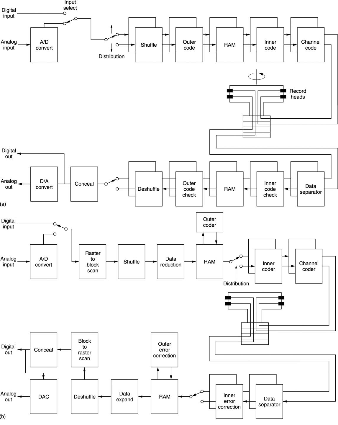
Figure 8.4(b) shows the block diagram of a DVTR using compression. Data from the convertors is rearranged from the normal raster scan to sets of pixel blocks upon which the compression unit works. A common size is eight pixels horizontally by four vertically. The blocks are then shuffled for concealment purposes. The shuffled blocks are passed through the data reduction unit. The output of this is distributed and then assembled into product codes and channel coded as for a conventional recorder. On replay, data separation and error-correcting take place as before, but there is now a matching compression decoder which outputs pixel blocks. These are then de-shuffled prior to the error-concealment stage. As concealment is more difficult with pixel blocks, data from another field may be employed for concealment as well as data within the field.

The various DVTR formats largely employ the same processing stages, but there are considerable differences in the order in which these are applied. Distribution is shown in Figure 8.5(a). This is a process of sharing the input bit rate over two or more signal paths so that the bit rate recorded in each is reduced. The data are subsequently recombined on playback. Each signal path requires its own tape track and head. The parallel tracks which result form a segment.

Figure 8.5 The fundamental stages of DVTR processing. At (a), distribution spreads data over more than one track to make concealment easier and to reduce the data rate per head. At (b) segmentation breaks video fields into manageable track lengths.

Figure 8.5 Product codes (c) correct mixture of random and burst errors. Correction failure requires concealment which may be in three dimensions as shown in (d). Irregular shuffle (e) makes concealments less visible.

Segmentation is shown in Figure 8.5(b). This is the process of sharing the data resulting from one video field over several segments. The replay system must have some means to ensure that associated segments are reassembled into the original field. This is generally a function of the control track.

Figure 8.5(c) shows a product code. Data to be recorded are protected by two error-correcting codeword systems at right-angles; the inner code and the outer code (see Chapter 6). When it is working within its capacity the error-correction system returns corrupt data to their original value and its operation is undetectable.

If errors are too great for the correction system, concealment will be employed. Concealment is the estimation of missing data values from surviving data nearby. Nearby means data on vertical, horizontal or time axes as shown in Figure 8.5(d). Concealment relies upon distribution, as all tracks of a segment are unlikely to be simultaneously lost, and upon the shuffle shown in Figure 8.5(e). Shuffling reorders the pixels prior to recording and is reversed on replay. The result is that uncorrectable errors due to dropouts are not concentrated, but are spread out by the de-shuffle, making concealment easier. A different approach is required where compression is used because the data recorded are not pixels representing a point, but coefficients representing an area of the image. In this case it is the DCT blocks (typically eight pixels across) which must be shuffled.

There are two approaches to error correction in segmented recordings. In D-1 and D-2 the approach shown in Figure 8.6(a) is used. Here, following distribution the input field is segmented first, then each segment becomes an independent shuffled product code. This requires less RAM to implement, but it means that from an error-correction standpoint each tape track is self-contained and must deal alone with any errors encountered.

Figure 8.6 Early formats would segment data before producing product codes as in (a). Later formats perform product coding first, and then segment for recording as in (b). This gives more robust performance.

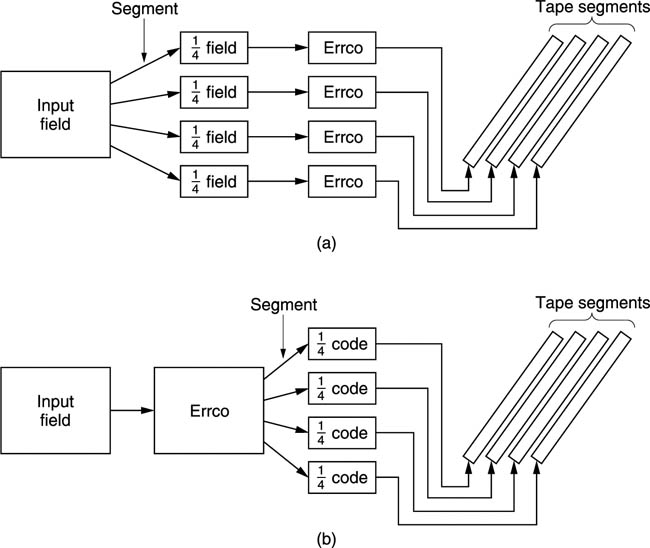
Later formats, beginning with D-3, use the approach shown in Figure 8.6(b). Here following distribution the entire field is used to produce one large shuffled product code in each channel. The product code is then segmented for recording on tape. Although more RAM is required to assemble the large product code, the result is that outer codewords on tape spread across several tracks and redundancy in one track can compensate for errors in another. The result is that size of a single burst error which can be fully corrected is increased. As the cost of RAM falls, this approach is becoming more common.

8.5 Operating modes of a DVTR

A simple recorder needs to do little more than record and play back, but the sophistication of modern production processes requires a great deal more flexibility. A production DVTR will need to support most if not all of the following:

8.6 Confidence replay

It is important to be quite certain that a recording is being made, and the only way of guaranteeing that this is so is actually to play the tape as it is being recorded. Extra heads are fitted to the revolving drum in such a way that they pass along the slant tracks directly behind the record heads. The drum must carry additional rotary transformers so that signals can simultaneously enter and leave the rotating head assembly. As can be seen in Figure 8.7, the input signal will be made available at the machine output if all is well. In analog machines it was traditional to assess the quality of the recording by watching a picture monitor connected to the confidence replay output during recording. With a digital machine this is not necessary, and instead the rate at which the replay channel performs error corrections should be monitored. In some machines the error rate is made available at an output socket so that remote or centralized data reliability logging can be used.

Figure 8.7 A professional DVTR uses confidence replay where the signal recorded is immediately played back. If the tape is not running, the heads are bypassed in E–E mode so that all of the circuitry can be checked.

It will be seen from Figure 8.7 that when the machine is not running, a connection is made which bypasses the record and playback heads. The output signal in this mode has passed through every process in the machine except the actual tape/head system. This is known as E–E (electronics to electronics) mode, and is a good indication that the circuitry is functioning.

8.7 Colour framing

Composite video has a subcarrier added to the luminance in order to carry the colour difference signals. The frequency of this subcarrier is critical if it is to be invisible on monochrome TV sets, and as a result it does not have a whole number of cycles within a frame, but only returns to its starting phase once every two frames in NTSC and every four frames in PAL. These are known as colour-framing sequences. When playing back a composite recording, the offtape colour-frame sequence must be synchronized with the reference colour-frame sequence, otherwise composite replay signals cannot be mixed with signals from elsewhere in the facility. When editing composite recordings, the subcarrier phase must not be disturbed at the edit point and this puts constraints on the edit control process. In both cases the solution is to record the start of a colour-frame sequence in the control track of the tape. There is also a standardised algorithm linking the timecode with the colour-framing sequences.

In practice many component formats have colour framing so that they can give better results when working with decoded composite signals.

8.8 Timecode

Timecode is simply a label attached to each frame on the tape which contains the time at which it was recorded measured in hours, minutes, seconds and frames. There are two ways in which timecode data can be recorded. The first is to use a dedicated linear track, usually alongside the control track, in which there is one timecode entry for every tape frame. Such a linear track can easily be played back over a wide speed range by a stationary head. Timecode of this kind is known as LTC (linear timecode).

LTC clearly cannot be replayed when the tape is stopped or moving very slowly. In DVTRs with track-following heads, particularly those which support preread, head deflection may result in a frame being played which is not the one corresponding to the timecode from the stationary head. The player software needs to modify the LTC value as a function of the head deflection.

An alternative timecode is where the information is recorded in the video field itself, so that the above mismatch cannot occur. This is known as vertical interval timecode (VITC) because it is recorded in a line which is in the vertical blanking period. VITC has the advantage that it can be recovered with the tape stopped, but it cannot be recovered in shuttle because the rotary heads do not play entire tracks in this mode. DVTRs do not record the whole of the vertical blanking period, and if VITC is to be used, it must be inserted in a line which is within the recorded data area of the format concerned.

8.9 Picture in shuttle

A rotary-head recorder cannot follow the tape tracks properly when the tape is shuttled. Instead the heads cross the tracks at an angle and intermittently pick up short data blocks. Each of these blocks is an inner error-correcting codeword and this can be checked to see if the block was properly recovered. If this is the case, the data can be used to update a framestore which displays the shuttle picture. Clearly, the shuttle picture is a mosaic of parts of many fields. In addition to helping the concealment of errors, the shuffle process is beneficial to obtaining picture-in-shuttle. Owing to shuffle, a block recovered from the tape contains data from many places in the picture, and this gives a better result than if many pixels were available from one place in the picture. The twinkling effect seen in shuttle is due to the updating of individual pixels following de-shuffle.

When compression is used, the picture is processed in blocks, and these will be visible as mosaicing in the shuttle picture as the framestore is updated by the blocks.

In composite recorders, the subcarrier sequence is only preserved when playing at normal speed. In all other cases, extra colour processing is required to convert the disjointed replay signal into a continuous subcarrier once more.

8.10 Digital Betacam

Digital Betacam (DB) is a component format which accepts eight- or ten-bit 4:2:2 data with 720 luminance samples per active line and four channels of 48 kHz digital audio having up to twenty-bit wordlength. Video compression based on the discrete cosine transform is employed, with a compression factor of almost two to one (assuming eight-bit input). The audio data are uncompressed. The cassette shell of the half-inch analog Betacam format is retained, but contains 14 micrometre metal particle tape. The digital cassette contains an identification hole which allows the transport to identify the tape type. Unlike the other digital formats, only two cassette sizes are available. The large cassette offers 124 minutes of playing time; the small cassette plays for 40 minutes.

Owing to the trade-off between SNR and bandwidth which is a characteristic of digital recording, the tracks must be longer than in the analog Betacam format, but narrower. The drum diameter of the DB transport is 81.4 mm which is designed to produce tracks of the required length for digital recording. The helix angle of the digital drum is designed such that when an analog Betacam tape is driven past at the correct speed, the track angle is correct. Certain DB machines are fitted with analog heads which can trace the tracks of an analog tape. As the drum size is different, the analog playback signal is time compressed by about 9 per cent, but this is easily dealt with in the timebase-correction process.1 The fixed heads are compatible with the analog Betacam positioning. The reverse compatibility is for playback only; the digital machine cannot record on analog cassettes.

Figure 8.8 shows the track pattern for 625/50 Betacam. The four digital audio channels are recorded in separate sectors of the slant tracks, and so one of the linear audio channels of the analog format is dispensed with, leaving one linear audio track for cueing.

Figure 8.8 The track pattern of Digital Betacam. Control and timecode tracks are identical in location to the analog format, as is the single analog audio cue track. Note the use of a small guard band between segments.

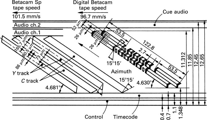
Azimuth recording is employed, with two tracks being recorded simultaneously by adjacent heads. Electronic delays are used to align the position of the edit gaps in the two tracks of a segment, allowing double-width flying-erase heads to be used. Three segments are needed to record one field, requiring one and a half drum revolutions. Thus the drum speed is three times that of the analog format. However, the track pitch is less than one third that of the analog format so the linear speed of the digital tape is actually slower. Track width is 24 micrometres, with a 4 micrometre guard band between segments making the effective track pitch 26 micrometres, compared with 18 for D-3/D-5 and 39 for D-2/DCT.

There is a linear timecode track whose structure is identical to the analog Betacam timecode, and a control track shown in Figure 8.9 having a fundamental frequency of 50 Hz. Ordinarily the duty cycle is 50 per cent, but this changes to 65/35 in field 1 and 35/65 in field 5. The rising edge of the CTL signal coincide with the first segment of a field, and the duty cycle variations allow four- or eight-field colour framing if decoded composite sources are used. As the drum speed is 75 Hz, CTL and drum phase coincide every three revolutions.

Figure 8.9 The control track of Digital Betacam uses duty cycle modulation for colour framing purposes.

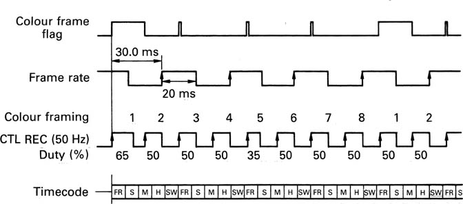
Figure 8.10 shows the track layout in more detail. Unlike earlier digital formats, DB incorporates tracking pilot tones recorded between the audio and video sectors. The first tone has a frequency of approximately 4 MHz and appears once per drum revolution. The second is recorded at approximately 400 kHz and appears twice per drum revolution. The pilot tones are recorded when a recording is first made on a blank tape, and will be rerecorded following an assemble edit, but during an insert edit the tracking pilots are not rerecorded, but used as a guide to the insertion of the new tracks.

Figure 8.10 The sector structure of Digital Betacam. Note the tracking tones between the audio and video sectors which are played back for alignment purposes during insert edits.

The amplitude of the pilot signal is a function of the head tracking. The replay heads are somewhat wider than the tracks, and so a considerable tracking error will have to be present before a loss of amplitude is noted. This is partly offset by the use of a very long wavelength pilot tone in which fringeing fields increase the effective track width. The low-frequency tones are used for automatic playback tracking.

With the tape moving at normal speed, the capstan phase is changed by steps in one direction then the other as the pilot tone amplitude is monitored. The phase which results in the largest amplitude will be retained. During the edit preroll the record heads play back the high-frequency pilot tone and capstan phase is set for largest amplitude. The record heads are the same width as the tracks and a short-wavelength pilot tone is used such that any mistracking will cause immediate amplitude loss. This is an edit optimize process and results in new tracks being inserted in the same location as the originals. As the pilot tones are played back in insert editing, there will be no tolerance build-up in the case of multiple inserts.

The compression technique of DB2 works on an intra-field basis to allow complete editing freedom and uses processes described in Chapter 5.

Figure 8.11 shows a block diagram of the record section of DB. Analog component inputs are sampled at 13.5 and 6.75 MHz. Alternatively the input may be SDI at 270 Mbits/s which is deserialized and demultiplexed to separate components. The raster scan input is first converted to blocks which are 8 pixels wide by 4 pixels high in the luminance channel and 4 pixels by 4 in the two colour difference channels. When two fields are combined on the screen, the result is effectively an interlaced 8 × 8 luminance block with colour difference pixels having twice the horizontal luminance pixel spacing. The pixel blocks are then subject to a field shuffle. A shuffle based on individual pixels is impossible because it would raise the high-frequency content of the image and destroy the power of the compression process. Instead the block shuffle helps the compression process by making the average entropy of the image more constant.

Figure 8.11 Block diagram of Digital Betacam record channel. Note that the use of data reduction makes this rather different to the block layout of full-bit formats.

This works because the shuffle exchanges blocks from flat areas of the image with blocks from highly detailed areas. The shuffle algorithm also has to consider the requirements of picture in shuttle. The blocking and shuffle take place when the read addresses of the input memory are permuted with respect to the write addresses.

Following the input shuffle the blocks are associated into sets of ten in each component and are then subject to the discrete cosine transform. The resulting coefficients are then subject to an iterative requantizing process followed by variable-length coding. The iteration adjusts the size of the quantizing step until the overall length of the ten coefficient sets is equal to the constant capacity of an entropy block which is 364 bytes. Within that entropy block the amount of data representing each individual DCT blocks may vary considerably, but the overall block size stays the same.

The DCT process results in coefficients whose wordlength exceeds the input wordlength. As a result it does not matter if the input wordlength is eight bits or ten bits; the requantizer simply adapts to make the output data rate constant. Thus the compression is greater with ten-bit input, corresponding to about 2.4 to 1.

The next step is the generation of product codes as shown in Figure 8.12(a). Each entropy block is divided into two halves of 162 bytes each and loaded into the rows of the outer code RAM which holds 114 such rows, corresponding to one twelfth of a field. When the RAM is full, it is read in columns by address mapping and 12 bytes of outer Reed–Solomon redundancy are added to every column, increasing the number of rows to 126.

Figure 8.12 Video product codes of Digital Betacam are shown in (a); twelve of these are needed to record one field. Audio product codes are shown in (b); two of these record samples corresponding to one field period. Sync blocks are common to audio and video as shown in (c). The ID code discriminates between video and audio channels.

The outer code RAM is read out in rows once more, but this time all 126 rows are read in turn. To the contents of each row is added a two-byte ID code and then the data plus ID bytes are turned into an inner code by the addition of 14 bytes of Reed–Solomon redundancy.

Inner codewords pass through the randomizer and are then converted to serial form for class-IV partial response precoding. With the addition of a sync pattern of two bytes, each inner codeword becomes a sync block as shown in Figure 8.12(c). Each video block contains 126 sync blocks, preceded by a preamble and followed by a postamble. One field of video data requires twelve such blocks. Pairs of blocks are recorded simultaneously by the parallel heads of a segment. Two video blocks are recorded at the beginning of the track, and two more are recorded after the audio and tracking tones.

The audio data for each channel are separated into odd and even samples for concealment purposes and assembled in RAM into two blocks corresponding to one field period. Two twenty-bit samples are stored in 5 bytes. Figure 8.12(b) shows that each block consists of 1458 bytes including auxiliary data from the AES/EBU interface, arranged as a block of 162 x 9 bytes. One hundred per cent outer code redundancy is obtained by adding 9 bytes of Reed–Solomon check bytes to each column of the blocks.

The inner codes for the audio blocks are produced by the same circuitry as the video inner codes on a time-shared basis. The resulting sync blocks are identical in size and differ only in the provision of different ID codes. The randomizer and precoder are also shared. It will be seen from Figure 8.10 that there are three segments in a field and that the position of an audio sector corresponding to a particular audio channel is different in each segment. This means that damage due to a linear tape scratch is distributed over three audio channels instead of being concentrated in one.

Each audio product block results in 18 sync blocks. These are accommodated in audio sectors of six sync blocks each in three segments. The audio sectors are preceded by preambles and followed by postambles. Between these are edit gaps which allow each audio channel to be independently edited.

By spreading the outer codes over three different audio sectors the correction power is much improved because data from two sectors can be used to correct errors in the third.

Figure 8.13 shows the replay channel of DB. The RF signal picked up by the replay head passes first to the Class IV partial response playback circuit in which it becomes a three-level signal as was shown in Chapter 6. The three-level signal is passed to an ADC which converts it into a digitally represented form so that the Viterbi detection can be carried out in logic circuitry. The sync detector identifies the synchronizing pattern at the beginning of each sync block and resets the block bit count. This allows the entire inner codeword of the sync block to be deserialized into bytes and passed to the inner error checker. Random errors will be corrected here, whereas burst errors will result in the block being flagged as in error.

Figure 8.13 The replay channel of Digital Betacam. This differs from a full-bit system primarily in the requirement to deserialize variable-length coefficient blocks prior to the inverse DCT.

Sync blocks are written into the de-interleave RAM with error flags where appropriate. At the end of each video sector the product code RAM will be filled, and outer code correction can be performed by reading the RAM at right-angles and using the error flags to initiate correction by erasure. Following outer code correction the RAM will contain corrected data or uncorrectable error flags which will later be used to initiate concealment.

The sync blocks can now be read from memory and assembled in pairs into entropy blocks. The entropy block is of fixed size, but contains coefficient blocks of variable length. The next step is to identify the individual coefficients and separate the luminance and colour difference coefficients by decoding the Huffman-coded sequence. Following the assembly of coefficient sets the inverse DCT will result in pixel blocks in three components once more. The pixel blocks are de-shuffled by mapping the write address of a field memory. When all the tracks of a field have been decoded, the memory will contain a de-shuffled field containing either correct sample data or correction flags. By reading the memory without address mapping the de-shuffled data are then passed through the concealment circuit where flagged data are concealed by data from nearby in the same field or from a previous field. The memory readout process is buffered from the offtape timing by the RAM and as a result the timebase correction stage is inherent in the replay process. Following concealment the data can be output as conventional raster-scan video either formatted to parallel or serial digital standards or converted to analog components.

8.11 DVC and DVCPRO

This component format uses quarter-inch wide metal evaporated (ME) tape which is only 7 micrometres thick in conjunction with compression to allow realistic playing times in miniaturized equipment. The format has jointly been developed by all the leading VCR manufacturers. Whilst intended as a consumer format it was clear that such a format is ideal for professional applications such as news gathering and simple production because of the low cost and small size. This led to the development of the DVCPRO format.

In addition to component video there are also two channels of sixteen-bit uniformly quantized digital audio at 32, 44.1 or 48 kHz, with an option of four audio channels using twelve-bit non-uniform quantizing at 32 kHz.

Figure 8.14 shows that two cassette sizes are supported. The standard size cassette offers 42 hours of recording time and yet is only a little larger than an audio Compact Cassette. The small cassette is even smaller than a DAT cassette yet plays for one hour. Machines designed to play both tape sizes will be equipped with moving-reel motors. Both cassettes are equipped with fixed identification tabs and a moveable write-protect tab. These tabs are sensed by switches in the transport.

Figure 8.14 The cassettes developed for the: ¼-inch DVC format. At (a) the standard cassette which holds 4.5 hours of program material.

Figure 8.14 The small cassette, shown at (b) is intended for miniature equipment and plays for 1 hour.

DVC (Digital Video Cassette) has adopted many of the features first seen in small formats such as the DAT digital audio recorder and the 8 mm analog video tape format. Of these the most significant is the elimination of the control track permitted by recording tracking signals in the slant tracks themselves. The adoption of metal evaporated tape and embedded tracking allows extremely high recording density. Tracks recorded with slant azimuth are only 10 μm wide and the minimum wavelength is only 0.!9 μm resulting in a superficial density of over 0.! Megabits per square millimetre.

Segmentation is used in DVC in such a way that as much commonality as possible exists between 50 and 60 Hz versions. The transport runs at 300 tape tracks per second; Figure 8.15 shows that 50 Hz frames contain 12 tracks and 60 Hz frames contain ten tracks.

The tracking mechanism relies upon buried tones in the slant tracks. From a tracking standpoint there are three types of track shown in Figure 8.16; F₀, F₁ and F₂. F₁ contains a low-frequency pilot and F₂ contains a high-frequency pilot. F₀ contains no pilot tone, but the recorded data spectrum contains notches at the frequencies of the two tones. Figure 8.16 also shows that every other track will contain F₀ following a four-track sequence.

Figure 8.15 In order to use a common transport for 50 and 60 Hz standards the segmentation shown here is used. The segment rate is constant but 10 or 12 segments can be used in a frame.

Figure 8.16 The tracks are of three types shown here. The F₀ track (a) contains spectral notches at two selected frequencies. The other two track types (b), (c) place a pilot tone in one or other of the notches.

The embedded tracking tones are recorded throughout the track by inserting a low frequency into the channel-coded data. Every twenty-four data bits an extra bit is added whose value has no data meaning but whose polarity affects the average voltage of the waveform. By controlling the average voltage with this bit, low frequencies can be introduced into the channel-coded spectrum to act as tracking tones. The tracking tones have sufficiently long wavelength that they are not affected by head azimuth and can be picked up by the ‘wrong’ head. When a head is following an F₀ type track, one edge of the head will detect F₁ and the other edge will detect F₂. If the head is centralized on the track, the amplitudes of the two tones will be identical. Any tracking error will result in the relative amplitudes of the F₁ F₂ tones changing. This can be used to modify the capstan phase in order to correct the tracking error. As azimuth recording is used requiring a minimum of two heads, one head of the pair will always be able to play a type F₀ track.

In simple machines only one set of heads will be fitted and these will record or play as required. In more advanced machines, separate record and replay heads will be fitted. In this case the replay head will read the tracking tones during normal replay, but in editing modes, the record head would read the tracking tones during the preroll in order to align itself with the existing track structure.

Figure 8.17 shows the track dimensions. The tracks are approximately 33mm long and lie at approximately 9° to the tape edge. A transport with a 180° wrap would need a drum of only 21 mm diameter. For camcorder applications with the small cassette this allows a transport no larger than an audio ‘Walkman’. With the larger cassette it would be advantageous to use time compression to allow a larger drum with partial wrap to be used. This would simplify threading and make room for additional heads in the drum for editing functions.

Figure 8.17 The dimensions of the DVC track. Audio, video and subcode can independently be edited. Insert and Track Information block aligns heads during insert.

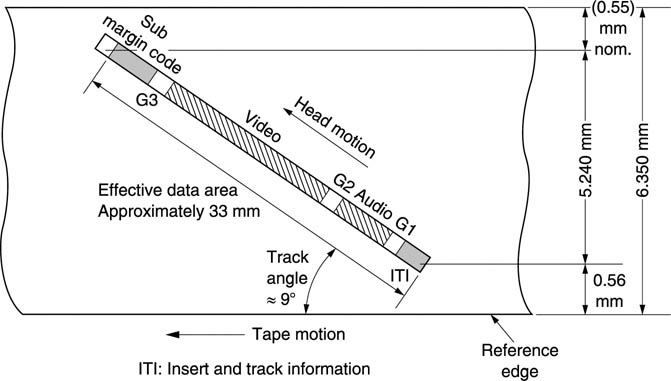
The audio, video and subcode data are recorded in three separate sectors with edit gaps between so that they can be independently edited in insert mode. In the case where all three data areas are being recorded in insert mode, there must be some mechanism to keep the new tracks synchronous with those which are being overwritten. In a conventional VTR this would be the job of the control track.

In DVC there is no control track and the job of tracking during insert is undertaken by part of each slant track. Figure 8.17 shows that the track begins with the insert and track information (ITI) block. During an insert edit the ITI block in each track is always read by the record head. This identifies the position of the track in the segmentation sequence and in the tracking tone sequence and allows the head to identify its physical position both along and across the track prior to an insert edit. The remainder of the track can then be recorded as required.

As there are no linear tracks, the subcode is designed to be read in shuttle for access control purposes. It will contain timecodes and flags.

Figure 8.18 shows a block diagram of the DVC signal system. The input video is eight-bit component digital according to CCIR-601, but compression of about 5:1 is used. The colour difference signals are subsampled prior to compression. In 60 Hz machines, 4:1:1 sampling is used, allowing a colour difference bandwidth in excess of that possible with NTSC. In 50 Hz machines, 4:2:0 sampling is used. The colour difference sampling rate is still 6.75 MHz, but the two colour difference signals are sent on sequential lines instead of simultaneously. The result is that the vertical colour difference resolution matches the horizontal resolution. A similar approach is used in SECAM and MAC video. Studio standard 4:2:2 parallel or serial inputs and outputs can be handled using simple interpolators in the colour difference signal paths.

Figure 8.18 Block diagram of DVC signal system. This is similar to larger formats except that a high compression factor allows use of a single channel with no distribution.

A 16:9 aspect ratio can be supported in standard definition by increasing the horizontal pixel spacing as is done in Digital Betacam. High-definition signals can be supported using a higher compression factor.

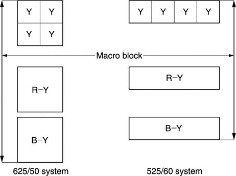
As in other DVTRs, the error-correction strategy relies upon a combination of shuffle and product codes. Frames are assembled in RAM, and partitioned into blocks of 8 × 8 pixels. In the luminance channel, four of these blocks cover the same screen area as one block in each colour difference signal as Figure 8.19 shows. The four luminance blocks and the two colour difference blocks are together known as a macroblock. The shuffle is based upon reordering of macroblocks. Following the shuffle compression takes place. The compression system is DCT based and uses techniques described in Chapter 5. Compression acts within frame boundaries so as to permit frame-accurate editing. This contrasts with the intra-field compression used in DB.

Figure 8.19 In DVC a macroblock contains information from a fixed screen area. As the colour resolution is reduced, there are twice as many luminance pixels.

Intra-frame compression uses 8 × 8 pixel DCT blocks and allows a higher compression factor because advantage can be taken of redundancy between the two fields when there is no motion. If motion is detected, then moving areas of the two fields will be independently coded in 8 × 4 pixel blocks to prevent motion blur. Following the motion compensation the DCT coefficients are weighted, zig-zag scanned and requantized prior to variable-length coding. As in other compressed VTR formats, the requantizing is adaptive so that the same amount of data is output irrespective of the input picture content. The entropy block occupies one sync block and contains data compressed from five macroblocks.

The DVC product codes are shown in Figure 8.20. The video product block is shown at (a). This block is common to both 525- and 625-line formats. Ten such blocks record one 525-line frame whereas 12 blocks are required for a 625-line frame.

Figure 8.20 The product codes used in DVC. Video and audio codes at (a) and (b) differ only in size and use the same inner code structure. Subcode at (c) is designed to be read in shuttle and uses short sync blocks to improve chances of recovery.

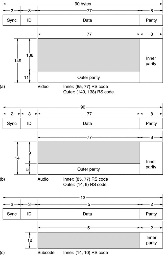
The audio channels are shuffled over a frame period and assembled into the product codes shown in Figure 8.20(b). Video and audio sync blocks are identical except for the ID numbering. The subcode structure is different. Figure 8.20(c) shows the structure of the subcode block. The subcode is not a product block because these can only be used for error correction when the entire block is recovered. The subcode is intended to be read in shuttle where only parts of the track are recovered. Accordingly only inner codes are used and these are much shorter than the video/audio codes, containing only 5 data bytes, known as a pack. The structure of a pack is shown In Figure 8.21. The subcode block in each track can accommodate 12 packs. Packs are repeated throughout the frame so that they have a high probability of recovery in shuttle. The pack header identifies the type of pack, leaving four bytes for pack data, e.g. timecode.

Figure 8.21 Structure of a pack.

Following the assembly of product codes, the data are then channel coded for recording on tape. A scrambled NRZI channel code is used which is similar to the system used in D-1 except that the tracking tones are also inserted by the modulation process.

In the DVCPRO format the extremely high recording density and long playing time of the consumer DVC was not a requirement. Instead ruggedness and reliable editing were needed. In developing DVCPRO, Panasonic chose to revert to metal particle tape as used in most other DVTRs. This requires wider tracks, and this was achieved by increasing the tape linear speed. The wider tracks also reduce the mechanical precision needed for interchange and editing. However, the DVCPRO transport can still play regular DVC tapes.

The DVCPRO format has proved to be extremely popular and a number of hard disk editors are now designed to import native DVCPRO data to cut down on generation loss. With a suitable tape drive this can be done at 4 χ normal speed. The SDTI interface (see Chapter 9) can also carry native DVC data.

8.12 The D-9 format

The D-9 format (formerly known as Digital-S) was developed by JVC and is based on half-inch metal particle tape. D-9 is intended as a fully specified 4:2:2 production format and so has four uncompressed 48 kHz digital audio tracks and a frame-based compression scheme with a mild compression factor.

In the same way that the Sony format used technology from the Betamax, the cassette and transport design of D-9 are refinements of the analog VHS format. Whereas the compression algorithm of Digital Betacam is unique, in D-9 the same algorithm as in DVC has been adopted. This gives an economic advantage as the DVC chip set is produced in large quantities. An increasing number of manufacturers are producing equipment which can accept native DVC-coded data to avoid generation loss and D-9 fits well with that concept.

In D-9 the bit rate on tape is 50 Mbits/s; twice that of the DVC format. As a result, the DCT coefficients will suffer less requantizing allowing a lower noise floor and genuine multi-generation performance. Tests performed by the EBU/SMPTE task force found that D-9 and Digital Betacam had almost identical performance.

8.13 Digital audio in VTRs

Digital audio recording with video is rather more difficult than in an audio-only environment. The audio samples are carried by the same channel as the video samples. The audio could have used separate stationary heads, but this would have increased tape consumption and machine complexity. In order to permit independent audio and video editing, the tape tracks are given a block structure. Editing will require the heads momentarily to go into record as the appropriate audio block is reached. Accurate synchronization is necessary if the other parts of the recording are to remain uncorrupted. The sync block structure of the video sector continues in the audio sectors because the same read/write circuitry is used for audio and video data. Clearly, the ID code structure must also continue through the audio. In order to prevent audio samples from arriving in the framestore in shuttle, the audio addresses are different from the video addresses.

Despite the additional complexity of sharing the medium with video, the professional DVTR must support such functions as track bouncing, synchronous recording and split audio edits with variable crossfade times.

The audio samples in a DVTR are binary numbers just like the video samples, and although there is an obvious difference in sampling rate and wordlength, the use of time compression means that this affects only the relative areas of tape devoted to the audio and video samples. The most important difference between audio and video samples is the tolerance to errors. The acuity of the ear means that uncorrected audio samples must not occur more than once every few hours. There is little redundancy in sound when compared to video, and concealment of errors is not desirable on a routine basis. In video, the samples are highly redundant, and concealment can be effected using samples from previous or subsequent lines or, with care, from the previous frame.

Whilst subjective considerations require greater data reliability in the audio samples, audio data form a small fraction of the overall data and it is difficult to protect them with an extensive interleave whilst still permitting independent editing. For these reasons major differences can be expected between the ways that audio and video samples are handled in a digital video recorder. One such difference is that the error-correction strategy for audio samples uses a greater amount of redundancy. Whilst this would cause a serious playing-time penalty in an audio recorder, even doubling the audio data rate in a video recorder only raises the overall data rate by a few per cent. The arrangement of the audio blocks is also designed to maximize data integrity in the presence of tape defects and head clogs. The audio blocks are at the ends of the head sweeps in D-2 and D-3, but are placed in the middle of the segment in D-1, D-5, Digital Betacam and DCT.

The audio sample interleave varies in complexity between the various formats. It will be seen from Figure 8.22 that the physical location of a given audio channel rotates from segment to segment. In this way a tape scratch will cause slight damage to all channels instead of serious damage to one. Data are also distributed between the heads, and so if one (or sometimes two) of the heads clogs, the audio is still fully recovered.

Figure 8.22 The structure of the audio blocks in D-1 format showing the double recording, the odd/even interleave, the sector addresses, and the distribution of audio channels over all heads. The audio samples recorded in this area represent a 6.666 ms time slot in the audio recording.

In each sector, the track commences with a preamble to synchronize the phase-locked loop in the data separator on replay. Each of the sync blocks begins, as the name suggests, with a synchronizing pattern which allows the read sequencer to deserialize the block correctly. At the end of a sector, it is not possible simply to turn off the write current after the last bit, as the turnoff transient would cause data corruption. It is necessary to provide a postamble such that current can be turned off away from the data. It should now be evident that any editing has to take place a sector at a time. Any attempt to rewrite one sync block would result in damage to the previous block owing to the physical inaccuracy of replacement, damage to the next block due to the turnoff transient, and inability to synchronize to the replaced block because of the random phase jump at the point where it began. The sector in a DVTR is analogous to the cluster in a disk drive. Owing to the difficulty of writing in exactly the same place as a previous recording, it is necessary to leave tolerance gaps between sectors where the write current can turn on and off to edit individual write blocks. For convenience, the tolerance gaps are made the same length as a whole number of sync blocks. Figure 8.23 shows that in D-1 the edit gap is two sync blocks long, as it is in D-3, whereas in D-2 it is only one sync block long. The first half of the tolerance gap is the postamble of the previous block, and the second half of the tolerance gap acts as the preamble for the next block. The tolerance gap following editing will contain, somewhere in the centre, an arbitrary jump in bit phase, and a certain amount of corruption due to turnoff transients. Provided that the postamble and preamble remain intact, this is of no consequence.

Figure 8.23 The position of preambles and postambles with respect to each sector is shown along with the gaps necessary to allow individual sectors to be written without corrupting others. When the whole track is recorded, 252 bytes of CC hex fill are recorded after the postamble before the next sync pattern. If a subsequent recording commences in this gap, it must do so at least 20 bytes before the end in order to write a new run-in pattern for the new recording.

The number of audio sync blocks in a given time is determined by the number of video fields in that time. It is only possible to have a fixed tape structure if the audio sampling rate is locked to video. With 625/50 machines, the sampling rate of 48 kHz results in exactly 960 audio samples in every field.

For use on 525/60, it must be recalled that the 60 Hz is actually 59.94 Hz. As this is slightly slow, it will be found that in sixty fields, exactly 48 048 audio samples will be necessary. Unfortunately 60 will not divide into 48 048 without a remainder. The largest number which will divide 60 and 48 048 is 12; thus in 60/12 = 5 fields there will be 48 048/12 = 4004 samples. Over a five-field sequence the fields contain 801, 801, 801, 801 and 800 samples respectively, adding up to 4004 samples.

8.14 AES/EBU compatibility

In order to comply with the AES/EBU digital audio interconnect, wordlengths between sixteen and twenty bits can be supported, but it is necessary to record a code in the sync block to specify the wordlength in use. Pre-emphasis may have been used prior to conversion, and this status is also to be conveyed, along with the four channel-use bits. The AES/EBU digital interconnect uses a block-sync pattern which repeats after 192 sample periods corresponding to 4ms at 48kHz. Since the block size is different to that of the DVTR interleave block, there can be any phase relationship between interleave-block boundaries and the AES/EBU block-sync pattern. In order to re-create the same phase relationship between block sync and sample data on replay, it is necessary to record the position of block sync within the interleave block. It is the function of the interface control word in the audio data to convey these parameters.

There is no guarantee that the 192-sample block-sync sequence will remain intact after audio editing; most likely there will be an arbitrary jump in block-sync phase. Strictly speaking, a DVTR, playing back an edited tape would have to ignore the block-sync positions on the tape, and create new block sync at the standard 192-sample spacing. Unfortunately the DVTR formats are not totally transparent to the whole of the AES/EBU data stream, as certain information is not recorded.

References

1. Huckfield, D., Sato, N. and Sato, I. Digital Betacam – The application of state of the art technology to the development of an affordable component DVTR. Record of 18th ITS, 180–199 (Montreux, 1993)

2. Creed, D. and Kaminaga, K. Digital compression strategies for video tape recorders in studio applications. Record of 18th ITS, 291–301 (Montreux, 1993)