Chapter 9

Digital communication

9.1 Introduction

Digital communication includes any system which can deliver data over distance. Figure 9.1 shows some of the ways in which the subject can be classified. The simplest is a unidirectional point-to-point signal path shown at (a). This is common in digital production equipment and includes the AES/EBU digital audio interface and the serial digital interface (SDI) for digital video. Bidirectional point-to-point signals include the RS-232 and RS-422 duplex systems. Bidirectional signal paths may be symmetrical, i.e. have the same capacity in both directions (b), or asymmetrical, having more capacity in one direction than the other (c). In this case the low-capacity direction may be known as a back channel.

Figure 9.1 Some ways of classifying communications systems. At (a) the unidirectional point-to-point connection used in many digital audio and video interconnects. (b) Symmetrical bidirectional point-to-point system. (c) Asymmetrical point-to-point system. (d) A network must have some switching or addressing ability in addition to delivering data. (e) Networks can be connected by gateways.

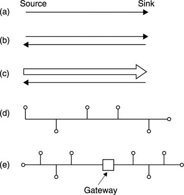
Back channels are useful in a number of applications. Video-on demand and interactive video are both systems in which the inputs from the viewer are relatively small, but result in extensive data delivery to the viewer. Archives and databases have similar characteristics.

When more than two devices can be interconnected in such a way that any one can communicate at will with any other, the result is a network as in Figure 9.1(d). The traditional telephone system is a network, and although the original infrastructure assumed analog speech transmission, subsequent developments in modems have allowed data transmission.

The computer industry has developed its own network technology, a long-serving example being Ethernet. Computer networks can work over various distances, giving rise to LANs (local area networks), MANs (metropolitan area networks) and WANs (wide area networks). Such networks can be connected together to form internetworks or internets for short, including the Internet. A private network, linking all employees of a given company, for example, may be referred to as an intranet.

Figure 9.1(e) shows that networks are connected together by gateways. In this example a private network (typically a local area network (LAN) within an office block) is interfaced to an access network (typically a metropolitan area network (MAN) with a radius of the order of a few kilometres) which in turn connects to the transport network. The access networks and the transport network together form a public network.

The different requirements of networks of different sizes have led to different protocols being developed. Where a gateway exists between two such networks, the gateway will often be required to perform protocol conversion. Protocol conversion represents unnecessary cost and delay and recent protocols such as ATM are sufficiently flexible that they can be adopted in any type of network to avoid conversion.

Networks also exist which are optimized for storage devices. These range from the standard buses linking hard drives with their controllers to SANs (storage area networks) in which distributed storage devices behave as one large store.

Communication must also include broadcasting, which initially was analog, but has also adopted digital techniques so that transmitters effectively radiate data. Traditional analog broadcasting was unidirectional, but with the advent of digital techniques, various means for providing a back channel have been developed.

To have an understanding of communications it is important to appreciate the concept of layers shown in Figure 9.2(a). The lowest layer is the physical medium dependent layer. In the case of a cabled interface, this layer would specify the dimensions of the plugs and sockets so that a connection could be made, and the use of a particular type of conductor such as co-axial, STP (screened twisted pair) or UTP (unscreened twisted pair). The impedance of the cable may also be specified. The medium may also be optical fibre which will need standardization of the terminations and the wavelength(s) in use.

Figure 9.2 (a) Layers are important in communications because they have a degree of independence such that one can be replaced by another leaving the remainder undisturbed. (b) The functions of a network protocol. See text.

Once a connection is made, the physical medium dependent layer standardizes the voltage of the transmitted signal and the frequency at which the voltage changes (the channel bit rate). This may be fixed at a single value, chosen from a set of fixed values, or, rarely, variable. Practical interfaces need some form of channel coding (see Chapter 6) in order to embed a bit clock in the data transmission.

The physical medium dependent layer allows binary transmission, but this needs to be structured or formatted. The transmission convergence layer takes the binary signalling of the physical medium dependent layer and builds a packet or cell structure. This consists at least of some form of synchronization system so that the start and end of serialized messages can be recognized and an addressing or labelling scheme so that packets can reliably be routed and recognized. Real cables and optical fibres run at fixed bit rates and a further function of the transmission convergence layer is the insertion of null or stuffing packets where insufficient user data exist.

In broadcasting, the physical medium dependent layer may be one which contains some form of radio signal and a modulation scheme. The modulation scheme will be a function of the kind of service, for example a satellite modulation scheme would be quite different from one used in a terrestrial service.

In all real networks requests for transmission will arise randomly. Network resources need to be applied to these requests in a structured way to prevent chaos, data loss or lack of throughput. This raises the requirement for a protocol layer. TCP (transmission control protocol) and ATM (asynchronous transfer mode) are protocols. A protocol is an agreed set of actions in given circumstances. In a point-to-point interface the protocol is trivial, but in a network it is complex. Figure 9.2(b) shows some of the functions of a network protocol. There must be an addressing mechanism so that the sender can direct the data to the desired location, and a mechanism by which the receiving device confirms that all the data have been correctly received. In more advanced systems the protocol may allow variations in quality of service whereby the user can select (and pay for) various criteria such as packet delay and delay variation and the packet error rate. This allows the system to deliver isochronous (near-real-time) MPEG data alongside asynchronous (non-time-critical) data such as e-mail by appropriately prioritizing packets.

The protocol layer arbitrates between demands on the network and delivers packets at the required quality of service. The user data will not necessarily have been packeted, or if they were the packet sizes may be different from those used in the network. This situation arises, for example, when MPEG transport packets are to be sent via ATM. The solution is to use an adaptation layer.

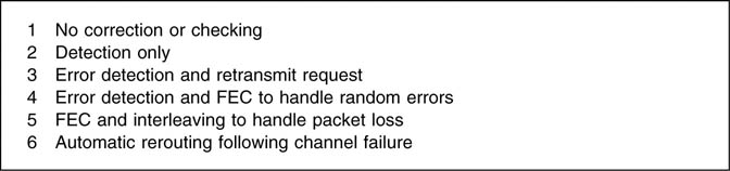
Adaptation layers reformat the original data into the packet structure needed by the network at the sending device, and reverse the process at the destination device. Practical networks must have error checking/correction. Figure 9.3 shows some of the possibilities. In short interfaces, no errors are expected and a simple parity check or checksum with an error indication is adequate. In bidirectional applications a checksum failure would result in a retransmission request or cause the receiver to fail to acknowledge the transmission so that the sender would try again. In real-time systems, there may not be time for a retransmission, and an FEC (forward error correction) system will be needed in which enough redundancy is included with every data block to permit on-the-fly correction at the receiver. The sensitivity to error is a function of the type of data, and so it is a further function of the adaptation layer to take steps such as interleaving and the addition of FEC codes.

Figure 9.3 Different approaches to error checking used in various communications systems.

9.2 Production-related interfaces

As audio and video production equipment made the transition from analog to digital technology, computers and networks were still another world and the potential of the digital domain was largely neglected because the digital interfaces which were developed simply copied analog practice but transmitted binary numbers instead of the original signal waveform. These interfaces are simple and have no addressing or handshaking ability. Creating a network requires switching devices called routers which are controlled independently of the signals themselves. Although obsolescent, there are substantial amounts of equipment in service adhering to these standards which will remain in use for some time.

The AES/EBU (Audio Engineering Society/European Broadcast Union) interface was developed to provide a short-distance point-to-point connection for PCM digital audio and subsequently evolved to handle compressed audio data.

The serial digital interface (SDI) was developed to allow up to ten-bit samples of standard definition interlaced component or composite digital video to be communicated serially.1 16:9 format component signals with 18 MHz sampling rate can also be handled. SDI as first standardized had no error-detection ability at all. This was remedied by a later option known as EDH (error detection and handling). The interface allows ancillary data including transparent conveyance of embedded AES/EBU digital audio channels during video blanking periods.

SDI is highly specific to two broadcast television formats. Subsequently the electrical and channel coding layer of SDI was used to create SDTI (serial data transport interface) which is used for transmitting, among other things, elementary streams from video compressors. ASI (asynchronous serial interface) uses only the electrical interface of SDI but with a different channel code and protocol and is used for transmitting MPEG transport streams through SDI-based equipment.

9.3 SDI

The serial digital interface was designed to allow easy conversion to and from traditional analog component video for production purposes. Only 525/59.94/2:1 and 625/50/2:1 formats are supported with 4:2:2 sampling. The sampling structure of SDI was detailed in section 7.14 and only the transmission technique will be considered here.

Chapter 6 introduced the concepts of DC components and uncontrolled clock content in serial data for recording and the same issues are important in interfacing, leading to a coding requirement. SDI uses convolutional randomizing, as shown in section 6.13, in which the signal sent down the channel is the serial data waveform which has been convolved with the impulse response of a digital filter. On reception the signal is deconvolved to restore the original data.

The components necessary for an SDI link are shown in Figure 9.4. Parallel component or composite data having a wordlength of up to ten bits form the input. These are fed to a ten-bit shift register which is clocked at ten times the input rate, which will be 270 MHz or 40 × F_sc. If there are only eight bits in the input words, the missing bits are forced to zero for transmission except for the all ones condition which will be forced to ten ones. The serial data from the shift register are then passed through the scrambler, in which a given bit is converted to the exclusive-OR of itself and two bits which are five and nine clocks ahead. This is followed by another stage, which converts channel ones into transitions. The resulting signal is fed to a line driver which converts the logic level into an alternating waveform of 800 mV peak-to-peak. The driver output impedance is carefully matched so that the signal can be fed down 75 Ohm co-axial cable using BNC connectors.

The scrambling process at the encoder spreads the signal spectrum and makes that spectrum reasonably constant and independent of the picture content. It is possible to assess the degree of equalization necessary by comparing the energy in a low-frequency band with that in higher frequencies. The greater the disparity, the more equalization is needed. Thus fully automatic cable equalization is easily achieved. The receiver must generate a bit clock at 270 MHz or 40 × F_sc from the input signal, and this clock drives the input sampler and slicer which converts the cable waveform back to serial binary. The local bit clock also drives a circuit which simply reverses the scrambling at the transmitter. The first stage returns transitions to ones, and the second stage is a mirror image of the encoder which reverses the exclusive-OR calculation to output the original data. Since transmission is serial, it is necessary to obtain word synchronization, so that correct deserialization can take place.

Figure 9.4 Major components of a serial scrambled link. Input samples are converted to serial form in a shift register clocked at ten times the sample rate. The serial data are then scrambled for transmission. On reception, a phase-locked loop recreates the bit rate clock and drives the de-scrambler and serial-to-parallel conversion. On detection of the sync pattern, the divide-by-ten counter is rephased to load parallel samples correctly into the latch. For composite working the bit rate will be 40 times subcarrier, and a sync pattern generator (top left) is needed to inject TRS-ID into the composite data stream.

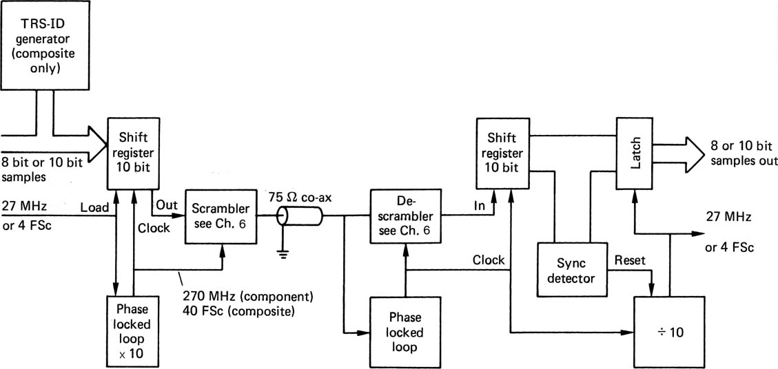
In the component parallel input, the SAV and EAV sync patterns are present and the all-ones and all-zeros bit patterns these contain can be detected in the thirty-bit shift register and used to reset the deserializer.

On detection of the synchronizing symbols, a divide-by-ten circuit is reset, and the output of this will clock words out of the shift register at the correct times. This output will also become the output word clock.

It is a characteristic of all randomizing techniques that certain data patterns will interact badly with the randomizing algorithm to produce a channel waveform which is low in clock content. These so-called pathological data patterns2 are extremely rare in real program material, but can be specially generated for testing purposes.

9.4 SDTI

SDI is closely specified and is only suitable for transmitting 2:1 interlaced 4:2:2 digital video in 525/60 or 625/50 systems. Since the development of SDI, it has become possible economically to compress digital video and the SDI standard cannot handle this. SDTI (serial data transport interface) is designed to overcome that problem by converting SDI into an interface which can carry a variety of data types whilst retaining compatibility with existing SDI router infrastructures.

SDTI3 sources produce a signal which is electrically identical to an SDI signal and which has the same timing structure. However, the digital active line of SDI becomes a data packet or item in SDTI. Figure 9.5 shows how SDTI fits into the existing SDI timing. Between EAV and SAV (horizontal blanking in SDI) an ancillary data block is incorporated. The structure of this meets the SDI standard, and the data within describe the contents of the following digital active line.

Figure 9.5 SDTI is a variation of SDI which allows transmission of generic data. This can include compressed video and non-real-time transfer.

The data capacity of SDTI is about 200Mbits/s because some of the 270 Mbits/s is lost due to the retention of the SDI timing structure. Each digital active line finishes with a CRCC (cyclic redundancy check character) to check for correct transmission.

SDTI raises a number of opportunities, including the transmission of compressed data at faster than real time. If a video signal is compressed at 4:1, then one quarter as much data would result. If sent in real time the bandwidth required would be one quarter of that needed by uncompressed video. However, if the same bandwidth is available, the compressed data could be sent in 1/4 of the usual time. This is particularly advantageous for data transfer between compressed camcorders and non-linear editing workstations. Alternatively, four different 50 Megabit/s signals could be conveyed simultaneously.

Thus an SDTI transmitter takes the form of a multiplexer which assembles packets for transmission from input buffers. The transmitted data can be encoded according to MPEG, MotionJPEG, Digital Betacam or DVC formats and all that is necessary is that compatible devices exist at each end of the interface. In this case the data are transferred with bit accuracy and so there is no generation loss associated with the transfer. If the source and destination are different, i.e. having different formats or, in MPEG, different group structures, then a conversion process with attendant generation loss would be needed.

9.5 ASI

The asynchronous serial interface is designed to allow MPEG transport streams to be transmitted over standard SDI cabling and routers. ASI offers higher performance than SDTI because it does not adhere to the SDI timing structure. Transport stream data do not have the same statistics as PCM video and so the scrambling technique of SDI cannot be used. Instead ASI uses an 8/10 group code (see section 6.12) to eliminate DC components and ensure adequate clock content).

SDI equipment is designed to run at a closely defined bit rate of 270 Mbits/s and has phase-locked loops in receiving and repeating devices which are intended to remove jitter. These will lose lock if the channel bit rate changes. Transport streams are fundamentally variable in bit rate and to retain compatibility with SDI routing equipment ASI uses stuffing bits to keep the transmitted bit rate constant.

The use of an 8/10 code means that although the channel bit rate is 270 Mbits/s, the data bit rate is only 80 per cent of that, i.e 216 Mbits/s. A small amount of this is lost to overheads.

9.6 AES/EBU

The AES/EBU digital audio interface, originally published in 19854 was proposed to embrace all the functions of existing formats in one standard. The goal was to ensure interconnection of professional digital audio equipment irrespective of origin. The EBU ratified the AES proposal with the proviso that the optional transformer coupling was made mandatory and led to the term AES/EBU interface, also called EBU/AES by some Europeans and standardized as IEC 958.

The interface has to be self-clocking and self-synchronizing, i.e. the single signal must carry enough information to allow the boundaries between individual bits, words and blocks to be detected reliably. To fulfil these requirements, the FM channel code is used (see Chapter 6) which is DC-free, strongly self-clocking and capable of working with a changing sampling rate. Synchronization of deserialization is achieved by violating the usual encoding rules.

The use of FM means that the channel frequency is the same as the bit rate when sending data ones. Tests showed that in typical analog audio-cabling installations, sufficient bandwidth was available to convey two digital audio channels in one twisted pair. The standard driver and receiver chips for RS–422A5 data communication (or the equivalent CCITT-V.11) are employed for professional use, but work by the BBC6 suggested that equalization and transformer coupling were desirable for longer cable runs, particularly if several twisted pairs occupy a common shield. Successful transmission up to 350 m has been achieved with these techniques.7 Figure 9.6 shows the standard configuration. The output impedance of the drivers will be about 110 Ohms, and the impedance of the cable and receiver should be similar at the frequencies of interest. The driver was specified in AES-3-1985 to produce between 3 and 10 V peak-to-peak into such an impedance but this was changed to between 2 and 7 V in AES-3-1992 to better reflect the characteristics of actual RS-422 driver chips.

Figure 9.6 Recommended electrical circuit for use with the standard two-channel interface.

In Figure 9.7, the specification of the receiver is shown in terms of the minimum eye pattern (see section 6.9) which can be detected without error. It will be noted that the voltage of 200 mV specifies the height of the eye opening at a width of half a channel bit period. The actual signal amplitude will need to be larger than this, and even larger if the signal contains noise. Figure 9.8 shows the recommended equalization characteristic which can be applied to signals received over long lines.

Figure 9.7 The minimum eye pattern acceptable for correct decoding of standard two-channel data.

Figure 9.8 EQ characteristic recommended by the AES to improve reception in the case of long lines.

The purpose of the standard is to allow the use of existing analog cabling, and as an adequate connector in the shape of the XLR is already in wide service, the connector made to IEC 268 Part 12 has been adopted for digital audio use. Effectively, existing analog audio cables having XLR connectors can be used without alteration for digital connections.

There is a separate standard8 for a professional interface using coaxial cable for distances of around 1000 m. This is simply the AES/EBU protocol but with a 75 Ohm coaxial cable carrying a one volt signal so that it can be handled by analog video distribution amplifiers. Impedance converting transformers allow balanced 110 Ohm to unbalanced 75 Ohm matching.

In Figure 9.9 the basic structure of the professional and consumer formats can be seen. One subframe consists of 32 bit-cells, of which four will be used by a synchronizing pattern. Subframes from the two audio channels, A and B, alternate on a time-division basis, with the least significant bit sent first. Up to twenty-four-bit sample wordlength can be used, which should cater for all conceivable future developments, but normally twenty-bit maximum length samples will be available with four auxiliary data bits, which can be used for a voice-grade channel in a professional application.

Figure 9.9 The basic subframe structure of the AES/EBU format. Sample can be twenty bits with four auxiliary bits, or twenty-four bits. LSB is transmitted first.

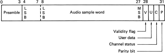
The format specifies that audio data must be in two’s complement coding. If different wordlengths are used, the MSBs must always be in the same bit position otherwise the polarity will be misinterpreted. Thus the MSB has to be in bit 27 irrespective of wordlength. Shorter words are leading-zero filled up to the twenty-bit capacity. The channel status data included from AES-3-1992 signalling of the actual audio wordlength used so that receiving devices could adjust the digital dithering level needed to shorten a received word which is too long or pack samples onto a storage device more efficiently.

Four status bits accompany each subframe. The validity flag will be reset if the associated sample is reliable. Whilst there have been many aspirations regarding what the Vbit could be used for, in practice a single bit cannot specify much, and if combined with other Vbits to make a word, the time resolution is lost. AES-3-1992 described the Vbit as indicating that the information in the associated subframe is ‘suitable for conversion to an analog signal’. Thus it might be reset if the interface was being used for non-PCM audio data such as the output of an audio compressor.

The parity bit produces even parity over the subframe, such that the total number of ones in the subframe is even. This allows for simple detection of an odd number of bits in error, but its main purpose is that it makes successive sync patterns have the same polarity, which can be used to improve the probability of detection of sync. The user and channel-status bits are discussed later.

Two of the subframes described above make one frame, which repeats at the sampling rate in use. The first subframe will contain the sample from channel A, or from the left channel in stereo working. The second subframe will contain the sample from channel B, or the right channel in stereo. At 48 kHz, the bit rate will be 3.072 MHz, but as the sampling rate can vary, the clock rate will vary in proportion.

In order to separate the audio channels on receipt the synchronizing patterns for the two subframes are different as Figure 9.10 shows. These sync patterns begin with a run length of 1.5 bits which violates the FM channel coding rules and so cannot occur due to any data combination. The type of sync pattern is denoted by the position of the second transition which can be 0.5, 1.0 or 1.5 bits away from the first. The third transition is designed to make the sync patterns DC-free.

Figure 9.10 Three different preambles (X, Y and Z) are used to synchronize a receiver at the start of subframes.

The channel status and user bits in each subframe form serial data streams with one bit of each per audio channel per frame. The channel status bits are given a block structure and synchronized every 192 frames, which at 48 kHz gives a block rate of 250 Hz, corresponding to a period of 4 ms. In order to synchronize the channel-status blocks, the channel A sync pattern is replaced for one frame only by a third sync pattern which is also shown in Figure 9.10. The AES standard refers to these as X, Y and Z whereas IEC 958 calls them M, W and B. As stated, there is a parity bit in each subframe, which means that the binary level at the end of a subframe will always be the same as at the beginning. Since the sync patterns have the same characteristic, the effect is that sync patterns always have the same polarity and the receiver can use that information to reject noise. The polarity of transmission is not specified, and indeed an accidental inversion in a twisted pair is of no consequence, since it is only the transition that is of importance, not the direction.

In both the professional and consumer formats, the sequence of channel-status bits over 192 subframes builds up a 24-byte channel-status block. However, the contents of the channel status data is completely different between the two applications. The professional channel status structure is shown in Figure 9.11. Byte 0 determines the use of emphasis and the sampling rate. Byte 1 determines the channel usage mode, i.e. whether the data transmitted are a stereo pair, two unrelated mono signals or a single mono signal, and details the user bit handling and byte 2 determines wordlength. Byte 3 is applicable only to multichannel applications. Byte 4 indicates the suitability of the signal as a sampling rate reference. There are two slots of four bytes each which are used for alphanumeric source and destination codes. These can be used for routing. The bytes contain seven-bit ASCII characters (printable characters only) sent LSB first with the eighth bit set to zero acording to AES-3–1992. The destination code can be used to operate an automatic router, and the source code will allow the origin of the audio and other remarks to be displayed at the destination.

Figure 9.11 Overall format of the professional channel-status block.

Bytes 14-17 convey a thirty-two-bit sample address which increments every channel status frame. It effectively numbers the samples in a relative manner from an arbitrary starting point. Bytes 18–21 convey a similar number, but this is a time-of-day count, which starts from zero at midnight. As many digital audio devices do not have real-time clocks built in, this cannot be relied upon. AES-3-92 specified that the time-of-day bytes should convey the real time at which a recording was made, making it rather like timecode. There are enough combinations in thirty-two bits to allow a sample count over 24 hours at 48 kHz. The sample count has the advantage that it is universal and independent of local supply frequency. In theory if the sampling rate is known, conventional hours, minutes, seconds, frames timecode can be calculated from the sample count, but in practice it is a lengthy computation and users have proposed alternative formats in which the data from EBU or SMPTE timecode are transmitted directly in these bytes. Some of these proposals are in service as de facto standards.

The penultimate byte contains four flags which indicate that certain sections of the channel-status information are unreliable. This allows the transmission of an incomplete channel-status block where the entire structure is not needed or where the information is not available. The final byte in the message is a CRCC which converts the entire channel-status block into a codeword (see Chapter 6). The channel status message takes 4 ms at 48 kHz and in this time a router could have switched to another signal source. This would damage the transmission, but will also result in a CRCC failure so the corrupt block is not used.

9.7 Telephone-based systems

The success of the telephone has led to vast number of subscribers being connected with copper wires and this is a valuable network infrastructure. As technology has developed, the telephone has become part of a global telecommunications industry. Simple economics suggests that in many cases improving the existing telephone cabling with modern modulation schemes is a good way of providing new communications services.

For economic reasons, there are fewer paths through the telephone system than there are subscribers. This is because telephones were not used continuously until teenagers discovered them. Before a call can be made, the exchange has to find a free path and assign it to the calling telephone. Traditionally this was done electromechanically. A path which was already in use would be carrying loop current. When the exchange sensed that a handset was off-hook, a rotary switch would advance and sample all the paths until it found one without loop current where it would stop. This was signalled to the calling telephone by sending a dial tone.

The development of electronics revolutionalized telephone exchanges. Whilst the loop current, AC ringing and hook switch sensing remained for compatibility, the electromechanical exchange gave way to electronic exchanges where the dial pulses were interpreted by digital counters which then drove crosspoint switches to route the call. The communication remained analog.

The next advance permitted by electronic exchanges was touch-tone dialling, also called DTMF. Touch-tone dialling is based on seven discrete frequencies shown in Figure 9.12. The telephone contains tone generators and tuned filters in the exchange can detect each frequency individually. The numbers 0 through 9 and two non-numerical symbols, asterisk and hash, can be transmitted using twelve unique tone pairs. A tone pair can reliably be detected in about 100 ms and this makes dialling much faster than the pulse system.

Figure 9.12 DTMF dialling works on tone pairs.

The frequencies chosen for DTMF are logarithmically spaced so that the filters can have constant bandwidth and response time, but they do not correspond to the conventional musical scale. In addition to dialling speed, because the DTMF tones are within the telephone audio bandwidth, they can also be used for signalling during a call.

The first electronic exchanges simply used digital logic to perform the routing function. The next step was to use a fully digital system where the copper wires from each subscriber terminate in an interface or line card containing ADCs and DACs. The sampling rate of 8 kHz retains the traditional analog bandwidth, and eight-bit quantizing is used. This is not linear, but uses logarithmically sized quantizing steps so that the quantizing error is greater on larger signals. The result is a 64 kbit/s data rate in each direction.

Packets of data can be time-division multiplexed into high bit-rate data buses which can carry many calls simultaneously. The routing function becomes simply one of watching the bus until the right packet comes along for the selected destination. 64 kbit/s data switching came to be known as IDN (Integrated Digital Network). As a data bus doesn’t care whether it carries 64 kbit/s of speech or 64 kbit/s of something else, communications systems based on IDN tend to be based on multiples of that rate.

Such a system is called ISDN (integrated services digital network) which is basically a use of the telephone system that allows dial-up data transfer between subscribers in much the same way as a conventional phone call is made.

With the subsequent development of broadband networks (B-ISDN) the original ISDN is now known as N-ISDN where the N stands for narrow-band. B-ISDN is the ultimate convergent network able to carry any type of data and uses the well-known ATM (asynchronous transfer mode) protocol. Broadband and ATM are considered in a later section.

One of the difficulties of the AMI coding used in N-ISDN are that the data rate is limited and new cabling is needed to the exchange. ADSL (asymmetric digital subscriber line) is an advanced coding scheme which obtains high bit rate delivery and a back channel down existing subscriber telephone wiring.

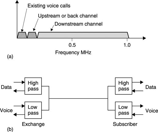
ADSL works on frequency-division multiplexing using 4 kHz wide channels, 249 of these provide the delivery or downstream channel and 25 provide the back channel. Figure 9.13(a) shows that the existing bandwidth used by the traditional analog telephone is retained. The back channel occupies the lowest-frequency channels, with the downstream channels above. Figure 9.13(b) shows that at each end of the existing telephone wiring a device called a splitter is needed. This is basically a high-pass/low-pass filter which directs audio frequency signals to the telephones and high-frequency signals to the modems.

Figure 9.13 (a) ADSL allows the existing analog telephone to be retained, but adds delivery and back channels at higher frequencies. (b) A splitter is needed at each end of the subscriber’s line.

Telephone wiring was never designed to support high-frequency signalling and is non-ideal. There will be reflections due to impedance mismatches which will cause an irregular frequency response in addition to high-frequency losses and noise which will all vary with cable length. ADSL can operate under these circumstances because it constantly monitors the conditions in each channel. If a given channel has adequate signal level and low noise, the full bit rate can be used, but in another channel there may be attenuation and the bit rate will have to be reduced. By independently coding the channels, the optimum data throughput for a given cable is obtained.

Each channel is modulated using DMT (discrete multitone technique) in which combinations of discrete frequencies are used. Within one channel symbol, there are 15 combinations of tones and so the coding achieves 15 bits/s/Hz. With a symbol rate of 4kHz, each channel can deliver 60kbits/s, making 14.9 Mbits/s for the downstream channel and 1.5 Mbits/s for the back channel. It should be stressed that these figures are theoretical maxima which are not reached in real cables. Practical ADSL systems deliver multiples of the ISDN channel rate up to about 6 Mbits/s, enough to deliver MPEG-2 coded video.

Over shorter distances, VDSL can reach up to 50 Mbits/s. Where ADSL and VDSL are being referred to as a common technology, the term xDSL will be found.

9.8 Digital television broadcasting

Digital television broadcasting relies on the combination of a number of fundamental technologies. These are: MPEG-2 compression to reduce the bit rate, multiplexing to combine picture and sound data into a common bitstream, digital modulation schemes to reduce the RF bandwidth needed by a given bit rate and error correction to reduce the error statistics of the channel down to a value acceptable to MPEG data.

MPEG compressed video is highly sensitive to bit errors, primarily because they confuse the recognition of variable length codes so that the decoder loses synchronization. However, MPEG is a compression and multiplexing standard and does not specify how error correction should be performed. Consequently a transmission standard must define a system which has to correct essentially all errors such that the delivery mechanism is transparent.

Essentially a transmission standard specifies all the additional steps needed to deliver an MPEG transport stream from one place to another. This transport stream will consist of a number of elementary streams of video and audio, where the audio may be coded according to MPEG audio standard or AC-3. In a system working within its capabilities, the picture and sound quality will be determined only by the performance of the compression system and not by the RF transmission channel.

Whilst in one sense an MPEG transport stream is only data, it differs from generic data in that it must be presented to the viewer at a particular rate. Generic data are usually asynchronous, whereas baseband video and audio are synchronous. However, after compression and multiplexing audio and video are no longer precisely synchronous and so the term isochronous is used. This means a signal that was at one time synchronous and will be displayed synchronously, but which uses buffering at transmitter and receiver to accommodate moderate timing errors in the transmission.

Clearly another mechanism is needed so that the time axis of the original signal can be re-created on reception. The time stamp and program clock reference system of MPEG does this.

Figure 9.14 shows that the concepts involved in digital television broadcasting exist at various levels which have an independence not found in analog technology. In a given configuration a transmitter can radiate a given payload data bit rate. This represents the useful bit rate and does not include the necessary overheads needed by error correction, multiplexing or synchronizing. It is fundamental that the transmission system does not care what this payload bit rate is used for. The entire capacity may be used up by one high-definition channel, or a large number of heavily compressed channels may be carried. The details of this data usage are the domain of the transport stream. The multiplexing of transport streams is defined by the MPEG standards, but these do not define any error-correction or transmission technique.

Figure 9.14 Source coder doesn’t know delivery mechanism and delivery doesn’t need to know what the data mean.

At the lowest level in Figure 9.15 the source coding scheme, in this case MPEG compression, results in one or more elementary streams, each of which carries a video or audio channel. Elementary streams are multiplexed into a transport stream. The viewer then selects the desired elementary stream from the transport stream. Metadata in the transport stream ensure that when a video elementary stream is chosen, the appropriate audio elementary stream will automatically be selected.

Figure 9.15 Program Specific Information helps the demultiplexer to select the required program.

9.9 MPEG packets and time stamps

The video elementary stream is an endless bitstream representing pictures which take a variable length of time to transmit. Bidirection coding means that pictures are not necessarily in the correct order. Storage and transmission systems prefer discrete blocks of data and so elementary streams are packetized to form a PES (packetized elementary stream). Audio elementary streams are also packetized. A packet is shown in Figure 9.16. It begins with a header containing an unique packet start code and a code which identifies the type of data stream. Optionally the packet header also may contain one or more time stamps which are used for synchronizing the video decoder to real time and for obtaining lip-sync.

Figure 9.16 A PES packet structure is used to break up the continuous elementary stream.

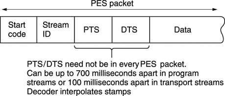
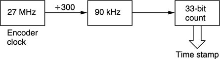
Figure 9.17 shows that a time stamp is a sample of the state of a counter which is driven by a 90 kHz clock. This is obtained by dividing down the master 27 MHz clock of MPEG-2. This 27 MHz clock must be locked to the video frame rate and the audio sampling rate of the program concerned. There are two types of time stamp: PTS and DTS. These are abbreviations for presentation time stamp and decode time stamp. A presentation time stamp determines when the associated picture should be displayed on the screen, whereas a decode time stamp determines when it should be decoded. In bidirectional coding these times can be quite different.

Figure 9.17 Time stamps are the result of sampling a counter driven by the encoder clock.

Audio packets have only presentation time stamps. Clearly if lip-sync is to be obtained, the audio sampling rate of a given program must have been locked to the same master 27 MHz clock as the video and the time stamps must have come from the same counter driven by that clock.

In practice, the time between input pictures is constant and so there is a certain amount of redundancy in the time stamps. Consequently PTS/DTS need not appear in every PES packet. Time stamps can be up to 100 ms apart in transport streams. As each picture type (I, P or B) is flagged in the bitstream, the decoder can infer the PTS/DTS for every picture from the ones actually transmitted.

The MPEG-2 transport stream is intended to be a multiplex of many TV programs with their associated sound and data channels, although a single program transport stream (SPTS) is possible. The transport stream is based upon packets of constant size so that multiplexing, adding error-correction codes and interleaving in a higher layer is eased. Figure 9.18 shows that these are always 188 bytes long.

Figure 9.18 Transport stream packets are always 188 bytes long to facilitate multiplexing and error correction.

Transport stream packets always begin with a header. The remainder of the packet carries data known as the payload. For efficiency, the normal header is relatively small, but for special purposes the header may be extended. In this case the payload gets smaller so that the overall size of the packet is unchanged. Transport stream packets should not be confused with PES packets which are larger and vary in size. PES packets are broken up to form the payload of the transport stream packets.

The header begins with a sync byte which is an unique pattern detected by a demultiplexer. A transport stream may contain many different elementary streams and these are identified by giving each an unique thirteen-bit Packet Identification Code or PID which is included in the header. A multiplexer seeking a particular elementary stream simply checks the PID of every packet and accepts only those which match.

In a multiplex there may be many packets from other programs in between packets of a given PID. To help the demultiplexer, the packet header contains a continuity count. This is a four-bit value which increments at each new packet having a given PID.

This approach allows statistical multiplexing as it does matter how many or how few packets have a given PID; the demux will still find them. Statistical multiplexing has the problem that it is virtually impossible to make the sum of the input bit rates constant. Instead the multiplexer aims to make the average data bit rate slightly less than the maximum and the overall bit rate is kept constant by adding ‘stuffing’ or null packets. These packets have no meaning, but simply keep the bit rate constant. Null packets always have a PID of 8191 (all ones) and the demultiplexer discards them.

9.10 Program clock reference

A transport stream is a multiplex of several TV programs and these may have originated from widely different locations. It is impractical to expect all the programs in a transport stream to be genlocked and so the stream is designed from the outset to allow unlocked programs. A decoder running from a transport stream has to genlock to the encoder and the transport stream has to have a mechanism to allow this to be done independently for each program. The synchronizing mechanism is called Program Clock Reference (PCR).

Figure 9.19 shows how the PCR system works. The goal is to re-create at the decoder a 27 MHz clock which is synchronous with that at the encoder. The encoder clock drives a forty-eight-bit counter which continuously counts up to the maximum value before overflowing and beginning again.

Figure 9.19 Program or System Clock Reference codes regenerate a clock at the decoder. See text for details.

A transport stream multiplexer will periodically sample the counter and place the state of the count in an extended packet header as a PCR (see Figure 9.18). The demultiplexer selects only the PIDs of the required program, and it will extract the PCRs from the packets in which they were inserted.

The PCR codes are used to control a numerically locked loop (NLL) described in section 2.9. The NLL contains a 27 MHz VCXO (voltage controlled crystal oscillator), a variable-frequency oscillator based on a crystal which has a relatively small frequency range.

The VCXO drives a forty-eight-bit counter in the same way as in the encoder. The state of the counter is compared with the contents of the PCR and the difference is used to modify the VCXO frequency. When the loop reaches lock, the decoder counter would arrive at the same value as is contained in the PCR and no change in the VCXO would then occur. In practice the transport stream packets will suffer from transmission jitter and this will create phase noise in the loop. This is removed by the loop filter so that the VCXO effectively averages a large number of phase errors.

A heavily damped loop will reject jitter well, but will take a long time to lock. Lockup time can be reduced when switching to a new program if the decoder counter is jammed to the value of the first PCR received in the new program. The loop filter may also have its time constants shortened during lockup.

Once a synchronous 27 MHz clock is available at the decoder, this can be divided down to provide the 90 kHz clock which drives the time stamp mechanism.

The entire timebase stability of the decoder is no better than the stability of the clock derived from PCR. MPEG-2 sets standards for the maximum amount of jitter which can be present in PCRs in a real transport stream.

Clearly, if the 27 MHz clock in the receiver is locked to one encoder it can only receive elementary streams encoded with that clock. If it is attempted to decode, for example, an audio stream generated from a different clock, the result will be periodic buffer overflows or underflows in the decoder. Thus MPEG defines a program in a manner which relates to timing. A program is a set of elementary streams which have been encoded with the same master clock.

9.11 Program Specific Information (PSI)

In a real transport stream, each elementary stream has a different PID, but the demultiplexer has to be told what these PIDs are and what audio belongs with what video before it can operate. This is the function of PSI which is a form of metadata. Figure 9.20 shows the structure of PSI. When a decoder powers up, it knows nothing about the incoming transport stream except that it must search for all packets with a PID of zero. PID zero is reserved for the Program Association Table (PAT). The PAT is transmitted at regular intervals and contains a list of all the programs in this transport stream. Each program is further described by its own Program Map Table (PMT) and the PIDs of of the PMTs are contained in the PAT.

Figure 9.20 also shows that the PMTs fully describe each program. The PID of the video elementary stream is defined, along with the PID(s) of the associated audio and data streams. Consequently when the viewer selects a particular program, the demultiplexer looks up the program number in the PAT, finds the right PMT and reads the audio, video and data PIDs. It then selects elementary streams having these PIDs from the transport stream and routes them to the decoders.

Figure 9.20 MPEG-2 Program Specific Information (PSI) is used to tell a demultiplexer what the transport stream contains.

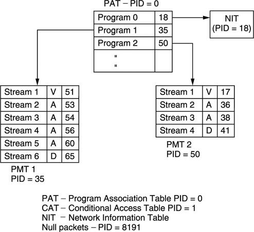
Program 0 of the PAT contains the PID of the Network Information Table (NIT). This contains information about what other transport streams are available. For example, in the case of a satellite broadcast, the NIT would detail the orbital position, the polarization, carrier frequency and modulation scheme. Using the NIT a set-top box could automatically switch between transport streams.

Apart from 0 and 8191, a PID of 1 is also reserved for the Conditional Access Table (CAT). This is part of the access control mechanism needed to support pay per view or subscription viewing.

9.12 Transport stream multiplexing

A transport stream multiplexer is a complex device because of the number of functions it must perform. A fixed multiplexer will be considered first. In a fixed multiplexer, the bit rate of each of the programs must be specified so that the sum does not exceed the payload bit rate of the transport stream. The payload bit rate is the overall bit rate less the packet headers and PSI rate.

In practice, the programs will not be synchronous to one another, but the transport stream must produce a constant packet rate given by the bit rate divided by 188 bytes, the packet length. Figure 9.21 shows how this is handled. Each elementary stream entering the multiplexer passes through a buffer which is divided into payload-sized areas. Note that periodically the payload area is made smaller because of the requirement to insert PCR.

Figure 9.21 A transport stream multiplexer can handle several programs which are asynchronous to one another and to the transport stream clock. See text for details.

MPEG-2 decoders also have a quantity of buffer memory. The challenge to the multiplexer is to take packets from each program in such a way that neither its own buffers nor the buffers in any decoder either overflow or underflow. This requirement is met by sending packets from all programs as evenly as possible rather than bunching together a lot of packets from one program. When the bit rates of the programs are different, the only way this can be handled is to use the buffer contents indicators. The more full a buffer is, the more likely it should be that a packet will be read from it. This a buffer content arbitrator can decide which program should have a packet allocated next.

If the sum of the input bit rates is correct, the buffers should all slowly empty because the overall input bit rate has to be less than the payload bit rate. This allows for the insertion of Program Specific Information. Whilst PATs and PMTs are being transmitted, the program buffers will fill up again. The multiplexer can also fill the buffers by sending more PCRs as this reduces the payload of each packet. In the event that the multiplexer has sent enough of everything but still can’t fill a packet then it will send a null packet with a PID of 8191. Decoders will discard null packets and as they convey no useful data, the multiplexer buffers will all fill whilst null packets are being transmitted.

The use of null packets means that the bit rates of the elementary streams do not need to be synchronous with one another or with the transport stream bit rate. As each elementary stream can have its own PCR, it is not necessary for the different programs in a transport stream to be genlocked to one another; in fact they don’t even need to have the same frame rate.

This approach allows the transport stream bit rate to be accurately defined and independent of the timing of the data carried. This is important because the transport stream bit rate determines the spectrum of the transmitter and this must not vary.

In a statistical multiplexer or statmux, the bit rate allocated to each program can vary dynamically. Figure 9.22 shows that there must be a tight connection between the statmux and the associated compressors. Each compressor has a buffer memory which is emptied by a demand clock from the statmux. In a normal, fixed bit rate, coder the buffer content feeds back and controls the requantizer. In statmuxing this process is less severe and only takes place if the buffer is very close to full, because the degree of coding difficulty is also fed to the statmux.

Figure 9.22 A statistical multiplexer contains an arbitrator which allocates bit rate to each program as a function of program difficulty.

The statmux contains an arbitrator which allocates more packets to the program with the greatest coding difficulty. Thus if a particular program encounters difficult material it will produce large prediction errors and begin to fill its output buffer. As the statmux has allocated more packets to that program, more data will be read out of that buffer, preventing overflow. Of course this is only possible if the other programs in the transport stream are handling typical video.

In the event that several programs encounter difficult material at once, clearly the buffer contents will rise and the requantizing mechanism will have to operate.

9.13 Broadcast modulation techniques

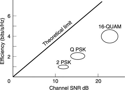
A key difference between analog and digital transmission is that the transmitter output is switched between a number of discrete states rather than continuously varying. A good code minimizes the channel bandwidth needed for a given bit rate. This quality of the code is measured in bits/s/Hz and is the equivalent of the density ratio in recording. Figure 9.23 shows, not surprisingly, that the less bandwidth required, the better the signal-to-noise ratio has to be. The figure shows the theoretical limit as well as the performance of a number of codes which offer different balances of bandwidth/noise performance.

Figure 9.23 Where a better SNR exists, more data can be sent down a given bandwidth channel.

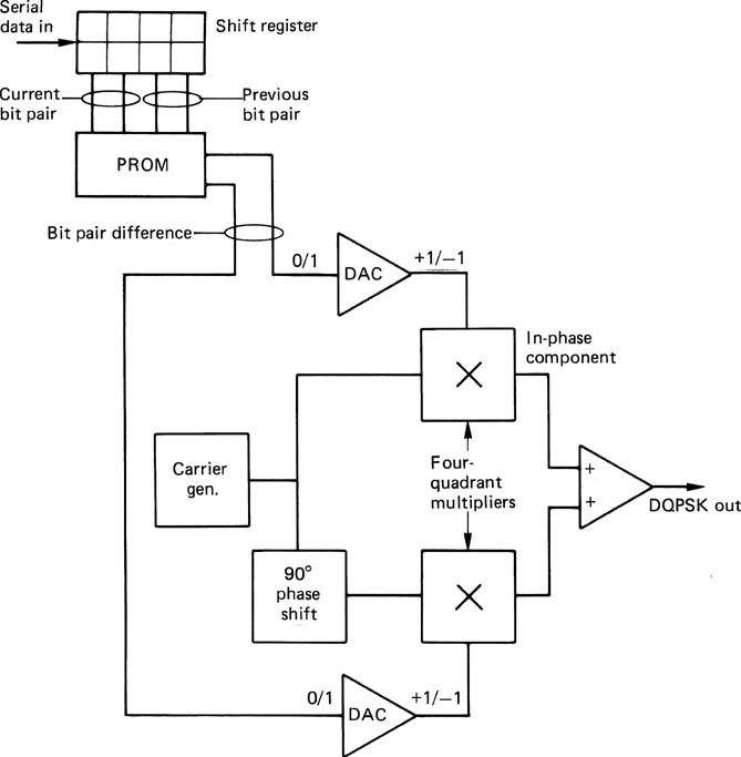
Where the SNR is poor, as in satellite broadcasting, the amplitude of the signal will be unstable, and phase modulation is used. Figure 9.24 shows that phaseshift keying (PSK) can use two or more phases. When four phases in quadrature are used, the result is Quadrature Phase Shift Keying or QPSK. Each period of the transmitted waveform can have one of four phases and therefore conveys the value of two data bits. 8-PSK uses eight phases and can carry three bits per symbol where the SNR is adequate. PSK is generally encoded in such a way that a knowledge of absolute phase is not needed at the receiver. Instead of encoding the signal phase directly, the data determine the magnitude of the phase shift between symbols. A QPSK coder is shown in Figure 9.25.

Figure 9.24 Differential quadrature phase shift keying (DQPSK).

Figure 9.25 A QPSK coder conveys two bits for each modulation period. See text for details.

In terrestrial transmission more power is available than, for example from a satellite and so a stronger signal can be delivered to the receiver. Where a better SNR exists, an increase in data rate can be had using multi-level signalling or m-ary coding instead of binary. Figure 9.26 shows that the ATSC system uses an eight-level signal (8-VSB) allowing three bits to be sent per symbol. Four of the levels exist with normal carrier phase and four with inverted phase so that a phase-sensitive rectifier is needed in the receiver. Clearly, the data separator must have a three-bit ADC which can resolve the eight signal levels. The gain and offset of the signal must be precisely set so that the quantizing levels register precisely with the centres of the eyes. The transmitted signal contains sync pulses which are encoded using specified code levels so that the data separator can set its gain and offset.

Figure 9.26 In 8-VSB the transmitter operates in eight different states enabling three bits to be sent per symbol.

Multi-level signalling systems have the characteristic that the bits in the symbol have different error probability. Figure 9.27 shows that a small noise level will corrupt the low-order bit, whereas twice as much noise will be needed to corrupt the middle bit and four times as much will be needed to corrupt the high-order bit. In ATSC the solution is that the lower two bits are encoded together in an inner error-correcting scheme so that they represent only one bit with similar reliability to the top bit. As a result the 8-VSB system actually delivers two data bits per symbol even though eight-level signalling is used.

Figure 9.27 In multi-level signalling the error probability is not the same for each bit.

The modulation of the carrier results in a double-sideband spectrum, but following analog TV practice most of the lower sideband is filtered off leaving a vestigial sideband only, hence the term 8-VSB. A small DC offset is injected into the modulator signal so that the four in-phase levels are slightly higher than the four out-of-phase levels. This has the effect of creating a small pilot at the carrier frequency to help receiver locking.

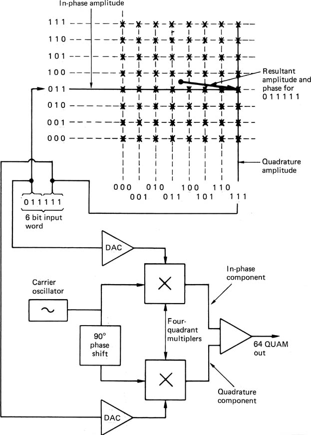
Multi-level signalling can be combined with PSK to obtain multi-level Quadrature Amplitude Modulation (QUAM). Figure 9.28 shows an example of 64-QUAM. Incoming six-bit data words are split into two three-bit words and each is used to amplitude modulate a pair of sinusoidal carriers which are generated in quadrature. The modulators are four-quadrant devices such that 2³ amplitudes are available, four which are in phase with the carrier and four which are antiphase. The two AM carriers are linearly added and the result is a signal which has 2⁶ or 64 combinations of amplitude and phase. There is a great deal of similarity between QUAM and the colour subcarrier used in analog television in which the two colour difference signals are encoded into one amplitudeand phase-modulated waveform. On reception, the waveform is sampled twice per cycle in phase with the two original carriers and the result is a pair of eight-level signals. 16-QUAM is also possible, delivering only four bits per symbol but requiring a lower SNR.

Figure 9.28 In 64-QUAM, two carriers are generated with a quadrature relationship. These are independently amplitude modulated to eight discrete levels in four quadrant multipliers. Adding the signals produces a QUAM signal having 64 unique combinations of amplitude and phase. Decoding requires the waveform to be sampled in quadrature like a colour TV subcarrier.

The data bit patterns to be transmitted can have any combinations whatsoever, and if nothing were done, the transmitted spectrum would be non-uniform. This is undesirable because peaks cause interference with other services, whereas energy troughs allow external interference in. The randomizing technique of section 6.13 is used to overcome the problem. The process is known as energy dispersal. The signal energy is spread uniformly throughout the allowable channel bandwidth so that it has less energy at a given frequency.

A pseudo-random sequence generator is used to generate the randomizing sequence. Figure 9.29 shows the randomizer used in DVB. This sixteen-bit device has a maximum sequence length of 65 535 bits, and is preset to a standard value at the beginning of each set of eight transport stream packets. The serialized data are XORed with the LSB of the Galois field, which randomizes the output which then goes to the modulator. The spectrum of the transmission is now determined by the spectrum of the prs.

Figure 9.29 (a) The randomizer of DVB is preset to the initial condition once every 8 transport stream packets. The maximum length of the sequence is 65 535 bits, but only the first 12 02! bits are used before resetting again (b).

9.14 OFDM

The way that radio signals interact with obstacles is a function of the relative magnitude of the wavelength and the size of the object. AM sound radio transmissions with a wavelength of several hundred metres can easily diffract around large objects. The shorter the wavelength of a transmission, the larger objects in the environment appear to it, and these objects can then become reflectors. Reflecting objects produce a delayed signal at the receiver in addition to the direct signal. In analog television transmissions this causes the familiar ghosting. In digital transmissions, the symbol rate may be so high that the reflected signal may be one or more symbols behind the direct signal, causing intersymbol interference. As the reflection may be continuous, the result may be that almost every symbol is corrupted. No error-correction system can handle this. Raising the transmitter power is no help at all as it simply raises the power of the reflection in proportion.

The only solution is to change the characteristics of the RF channel in some way to either prevent the multipath reception or stop it being a problem. The RF channel includes the modulator, transmitter, antennae, receiver and demodulator.

As with analog UHF TV transmissions, a directional antenna is useful with digital transmission as it can reject reflections. However, directional antennae tend to be large and they require a skilled permanent installation. Mobile use on a vehicle or vessel is simply impractical.

Another possibility is to incorporate a ghost canceller in the receiver. The transmitter periodically sends a standardized waveform known as a training sequence. The receiver knows what this waveform looks like and compares it with the received signal. In theory it is possible for the receiver to compute the delay and relative level of a reflection and so insert an opposing one. In practice if the reflection is strong it may prevent the receiver finding the training sequence.

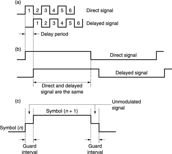
The most elegant approach is to use a system in which multipath reception conditions cause only a small increase in error rate which the error-correction system can manage. This approach is used in DVB. Figure 9.30(a) shows that when using one carrier with a high bit rate, reflections can easily be delayed by one or more bit periods, causing interference between the bits. Figure 9.30(b) shows that instead, OFDM sends many carriers each having a low bit rate. When a low bit rate is used, the energy in the reflection will arrive during the same bit period as the direct signal. Not only is the system immune to multipath reflections, but the energy in the reflections can actually be used. This characteristic can be enhanced by using guard intervals shown in Figure 9.30(c). These reduce multipath bit overlap even more.

Figure 9.30 (a) High bit rate transmissions are prone to corruption due to reflections. (b) If the bit rate is reduced the effect of reflections is eliminated, in fact reflected energy can be used. (c) Guard intervals may be inserted between symbols.

Note that OFDM is not a modulation scheme, and each of the carriers used in a OFDM system still needs to be modulated using any of the digital coding schemes described above. What OFDM does is to provide an efficient way of packing many carriers close together without mutual interference.

A serial data waveform basically contains a train of rectangular pulses. The transform of a rectangle is the function sinx/x and so the baseband pulse train has a sinx/x spectrum. When this waveform is used to modulate a carrier the result is a symmetrical sinx/x spectrum centred on the carrier frequency. Figure 9.31(a) shows that nulls in the spectrum appear spaced at multiples of the bit rate away from the carrier.

Figure 9.31 In OFDM the carrier spacing is critical, but when correct the carriers become independent and most efficient use is made of the spectrum. (a) Spectrum of bitstream has regular nulls. (b) Peak of one carrier occurs at null of another.

Further carriers can be placed at spacings such that each is centred at the nulls of the others as is shown in Figure 9.31(b). The distance between the carriers is equal to 90° or one quadrant of sinx. Owing to the quadrant spacing, these carriers are mutually orthogonal, hence the term ‘orthogonal frequency division’. A large number of such carriers (in practice, several thousand) will be interleaved to produce an overall spectrum which is almost rectangular and which fills the available transmission channel.

When guard intervals are used, the carrier returns to an unmodulated state between bits for a period which is greater than the period of the reflections. Then the reflections from one transmitted bit decay during the guard interval before the next bit is transmitted. The use of guard intervals reduces the bit rate of the carrier because for some of the time it is radiating carrier, not data. A typical reduction is to around 80 per cent of the capacity without guard intervals.

This capacity reduction does, however, improve the error statistics dramatically, such that much less redundancy is required in the error-correction system. Thus the effective transmission rate is improved. The use of guard intervals also moves more energy from the sidebands back to the carrier. The frequency spectrum of a set of carriers is no longer perfectly flat but contains a small peak at the centre of each carrier.

The ability to work in the presence of multipath cancellation is one of the great strengths of OFDM. In DVB, more than 2000 carriers are used in single-transmitter systems. Provided there is exact synchronism, several transmitters can radiate exactly the same signal so that a single-frequency network can be created throughout a whole country. SFNs require a variation on OFDM which uses over 8000 carriers.

With OFDM, directional antennae are not needed and, given sufficient field strength, mobile reception is perfectly feasible. Of course, directional antennae may still be used to boost the received signal outside of normal service areas or to enable the use of low-powered transmitters.

An OFDM receiver must perform fast Fourier transforms (FFTs) on the whole band at the symbol rate of one of the carriers. The amplitude and/or phase of the carrier at a given frequency effectively reflects the state of the transmitted symbol at that time slot and so the FFT partially demodulates as well.

In order to assist with tuning in, the OFDM spectrum contains pilot signals. These are individual carriers which are transmitted with slightly more power than the remainder. The pilot carriers are spaced apart through the whole channel at agreed frequencies which form part of the transmission standard.

Practical reception conditions, including multipath reception, will cause a significant variation in the received spectrum and some equalization will be needed. Figure 9.32 shows what the possible spectrum looks like in the presence of a powerful reflection. The signal has almost been cancelled at certain frequencies. However, the FFT performed in the receiver is effectively a spectral analysis of the signal and so the receiver computes for free the received spectrum. As in a flat spectrum the peak magnitude of all the coefficients would be the same (apart from the pilots), equalization is easily performed by multiplying the coefficients by suitable constants until this characteristic is obtained.

Figure 9.32 Multipath reception can place notches in the channel spectrum. This will require equalization at the receiver.

Although the use of transform-based receivers appears complex, when it is considered that such an approach simultaneously allows effective equalization the complexity is not significantly higher than that of a conventional receiver which needs a separate spectral analysis system just for equalization purposes.

The only drawback of OFDM is that the transmitter must be highly linear to prevent intermodulation between the carriers. This is readily achieved in terrestrial transmitters by derating the transmitter so that it runs at a lower power than it would in analog service. This is not practicable in satellite transmitters which are optimized for efficiency so OFDM is not really suitable for satellite use.

9.15 Error correction in digital television broadcasting

As in recording, broadcast data suffer from both random and burst errors and the error-correction strategies of digital television broadcasting have to reflect that. Figure 9.33 shows a typical system in which inner and outer codes are employed. The Reed–Solomon codes are universally used for burst-correcting outer codes, along with an interleave which will be convolutional rather than the block-based interleave used in recording media. The inner codes will not be R–S, as more suitable codes exist for the statistical conditions prevalent in broadcasting. DVB uses a parity-based variable-rate system in which the amount of redundancy can be adjusted according to reception conditions. ATSC uses a fixed-rate parity-based system along with trellis coding to overcome co-channel interference from analog NTSC transmitters.

Figure 9.33 Error-correcting strategy of digital television broadcasting systems.

9.16 DVB

The DVB system is subdivided into systems optimized for satellite, cable and terrestrial delivery. This section concentrates on the terrestrial delivery system. Figure 9.34 shows a block diagram of a DVB-T transmitter.

Figure 9.34 DVB-T transmitter block diagram. See text for details.

Incoming transport stream packets of 188 bytes each are first subject to R-S outer coding. This adds 16 bytes of redundancy to each packet, resulting in 204 bytes. Outer coding is followed by interleaving. The interleave mechanism is shown in Figure 9.35. Outer code blocks are commutated on a byte basis into twelve parallel channels. Each channel contains a different amount of delay, typically achieved by a ring-buffer RAM. The delays are integer multiples of 17 bytes, designed to skew the data by one outer block (12 × 17 = 204). Following the delays, a commutator reassembles interleaved outer blocks. These have 204 bytes as before, but the effect of the interleave is that adjacent bytes in the input are 17 bytes apart in the output. Each output block contains data from twelve input blocks making the data resistant to burst errors.

Figure 9.35 The interleaver of DVB uses 12 incrementing delay channels to reorder the data. The sync byte passes through the undelayed channel and so is still at the head of the packet after interleave. However, the packet now contains non-adjacent bytes from 12 different packets.

Following the interleave, the energy-dispersal process takes place. The pseudo-random sequence runs over eight outer blocks and is synchronized by inverting the transport stream packet sync symbol in every eighth block. The packet sync symbols are not randomized.

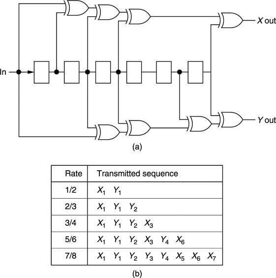
The inner coding process of DVB is shown in Figure 9.36. Input data are serialized and pass down a shift register. Exclusive-OR gates produce convolutional parity symbols X and Y, such that the output bit rate is twice the input bit rate. Under the worst reception conditions, this 100 per cent redundancy offers the most powerful correction with the penalty that a low data rate is delivered. However, Figure 9.36 also shows that a variety of inner redundancy factors can be used from 1/2 down to 1/8 of the transmitted bit rate. The X, Y data from the inner coder are subsampled, such that the coding is punctured.

Figure 9.36 (a) The mother inner coder of DVB produces 100 per cent redundancy, but this can be punctured by subsampling the X and Y data to give five different code rates as (b) shows.

The DVB standard allows the use of QPSK, 16-QUAM or 64-QUAM coding in an OFDM system. There are five possible inner code rates, and four different guard intervals which can be used with each modulation scheme, Thus for each modulation scheme there are twenty possible transport stream bit rates in the standard DVB channel, each of which requires a different receiver SNR. The broadcaster can select any suitable balance between transport stream bit rate and coverage area. For a given transmitter location and power, reception over a larger area may require a channel code with a smaller number of bits/s/Hz and this reduces the bit rate which can be delivered in a standard channel. Alternatively a higher amount of inner redundancy means that the proportion of the transmitted bit rate which is data goes down. Thus for wider coverage the broadcaster will have to send fewer programs in the multiplex or use higher compression factors.

Figure 9.37 shows a block diagram of a DVB receiver. The off-air RF signal is fed to a mixer driven by the local oscillator. The IF output of the mixer is bandpass filtered and supplied to the ADC which outputs a digital IF signal for the FFT stage. The FFT is analysed initially to find the higher-level pilot signals. If these are not in the correct channels the local oscillator frequency is incorrect and it will be changed until the pilots emerge from the FFT in the right channels. The data in the pilots will be decoded in order to tell the receiver how many carriers, what inner redundancy rate, guard band rate and modulation scheme are in use in the remaining carriers. The FFT magnitude information is also a measure of the equalization required.

Figure 9.37 DVB receiver block diagram. See text for details.

The FFT outputs are demodulated into 2K or 8K bitstreams and these are multiplexed to produce a serial signal. This is subject to inner error correction which corrects random errors. The data are then de-interleaved to break up burst errors and then the outer R–S error-correction operates. The output of the R–S correction will then be derandomized to become an MPEG transport stream once more. The derandomizing is synchronized by the transmission of inverted sync patterns.

The receiver must select a PID of 0 and wait until a Program Association Table (PAT) is transmitted. This will describe the available programs by listing the PIDs of the Program Map Tables (PMT). By looking for these packets the receiver can determine what PIDs to select to receive any video and audio elementary streams.

When an elementary stream is selected, some of the packets will have extended headers containing program clock reference (PCR). These codes are used to synchronize the 27 MHz clock in the receiver to the one in the MPEG encoder of the desired program. The 27 MHz clock is divided down to drive the time stamp counter so that audio and video emerge from the decoder at the correct rate and with lip sync.

It should be appreciated that time stamps are relative, not absolute. The time stamp count advances by a fixed amount each picture, but the exact count is meaningless. Thus the decoder can only establish the frame rate of the video from time stamps, but not the precise timing. In practice the receiver has finite buffering memory between the demultiplexer and the MPEG decoder. If the displayed video timing is too late, the buffer will tend to overflow whereas if the displayed video timing is too early the decoding may not be completed. The receiver can advance or retard the time stamp counter during lockup so that it places the output timing mid-way between these extremes.

9.17 ATSC

The ATSC system is an alternative way of delivering a transport stream, but it is considerably less sophisticated than DVB, and supports only one transport stream bit rate of 19.28 Mbits/s. If any change in the service area is needed, this will require a change in transmitter power.

Figure 9.38 shows a block diagram of an ATSC transmitter. Incoming transport stream packets are randomized, except for the sync pattern, for energy dispersal. Figure 9.39 shows the randomizer.

Figure 9.38 Block diagram of ATSC transmitter. See text for details.

Figure 9.39 The randomizer of ATSC. The twisted ring counter is preset to the initial state shown each data field. It is then clocked once per byte and the eight outputs D₀-D₇ are X-ORed with the data byte.

The outer correction code includes the whole packet except for the sync byte. Thus there are 187 bytes of data in each codeword. Twenty bytes of R-S redundancy are added to make a 207-byte codeword. After outer coding, a convolutional interleaver shown in Figure 9.40 is used. This reorders data over a time span of about 4 ms. Interleave simply exchanges content between packets, but without changing the packet structure.

Figure 9.40 The ATSC convolutional interleaver spreads adjacent bytes over a period of about 4 ms.

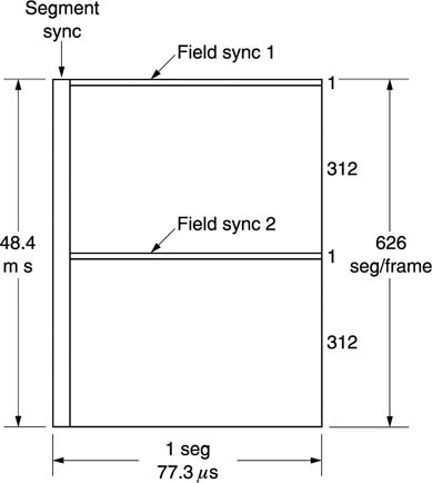
Figure 9.41 shows that the result of outer coding and interleave is a data frame which is divided into two fields of 313 segments each. The frame is tranmitted by scanning it horizontally a segment at a time. There is some similarity with a traditional analog video signal here, because there is a sync pulse at the beginning of each segment and a field sync which occupies two segments of the frame. Data segment sync repeats every 77.3 ms, a segment rate of 12933 Hz, whereas a frame has a period of 48.4ms. The field sync segments contain a training sequnce to drive the adaptive equalizer in the receiver.

Figure 9.41 The ATSC data frame is transmitted one segment at a time. Segment sync denotes the beginning of each segment and the segments are counted from the field sync signals.

The data content of the frame is subject to trellis coding which converts each pair of data bits into three channel bits inside an inner interleave. The trellis coder is shown in Figure 9.42 and the interleave in Figure 9.43. Figure 9.42 also shows how the three channel bits map to the eight signal levels in the 8-VSB modulator.

Figure 9.42 (a) The precoder and trellis coder of ATSC converts two data bits X₁, X₂ to three output bits Z₀, Z₁, Z₂. (b) The Z₀, Z₁, Z₂ output bits map to the eight-level code as shown.

Figure 9.43 The inner interleave (a) of ATSC makes the trellis coding operate as twelve parallel channels working on every twelfth byte to improve error resistance. The interleave is byte-wise, and, as (b) shows, each byte is divided into four di-bits for coding into the tri-bits Z₀, Z₁, Z₂.

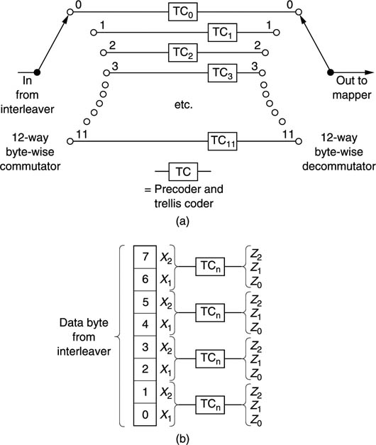
Figure 9.44 shows the data segment after eight-level coding. The sync pattern of the transport stream packet, which was not included in the error-correction code, has been replaced by a segment sync waveform. This acts as a timing reference to allow deserializing of the segment, but as the two levels of the sync pulse are standardized, it also acts as an amplitude reference for the eight-level slicer in the receiver.

Figure 9.44 ATSC data segment. Note the sync pattern which acts as a timing and amplitude reference. The eight levels are shifted up by 1.25 to create a DC component resulting in a pilot at the carrier frequency.

The eight-level signal is subject to a DC offset so that some transmitter energy appears at the carrier frequency to act as a pilot. Each eight-level symbol carries two data bits and so there are 832 symbols in each segment. As the segment rate is 12 933 Hz, the symbol rate is 10.76 MHz and so this will require 5.38 MHz of bandwidth in a single sideband,

Figure 9.45 shows the transmitter spectrum. The lower sideband is vestigial and an overall channel width of 6 MHz results.

Figure 9.45 The spectrum of ATSC and its associated bit and symbol rates. Note pilot at carrier frequency created by DC offset in multi-level coder.

Figure 9.46 shows an ATSC receiver. The first stages of the receiver are designed to lock to the pilot in the transmitted signal. This then allows the eight-level signal to be sampled at the right times. This process will allow location of the segment sync and then the field sync signals. Once the receiver is synchronized, the symbols in each segment can be decoded. The inner or trellis coder corrects for random errors, then following de-interleave the R–S coder corrects burst errors, After derandomizing, standard transport stream sync patterns are added to the output data.

Figure 9.46 An ATSC receiver. Double conversion can be used so that the second conversion stage can be arranged to lock to the transmitted pilot.

In practice, ATSC transmissions will experience co-channel interference from NTSC transmitters and the ATSC scheme allows the use of an NTSC rejection filter. Figure 9.47 shows that most of the energy of NTSC is at the carrier, subcarrier and sound carrier frequencies. A comb filter with a suitable delay can produce nulls or notches at these frequencies. However, the delay-and-add process in the comb filter also causes another effect. When two eight-level signals are added together, the result is a sixteen-level signal. This will be corrupted by noise of half the level that would corrupt an eight-level signal. However, the sixteen-level signal contains redundancy because it corresponds to the combinations of four bits whereas only two bits are being transmitted. This allows a form of error correction to be used.

Figure 9.47 Spectrum of typical analog transmitter showing (a) maximum power at carrier, subcarrier and audio carrier. A comb filter (b) with a suitable delay can notch out NTSC interference. The precoding of ATSC is designed to work with the necessary receiver delay.

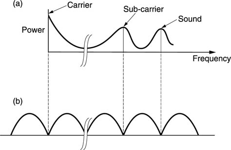
The ATSC inner precoder results in a known relationship existing between symbols independent of the data. The time delays in the inner interleave are designed to be compatible with the delay in the NTSC rejection comb filter. This limits the number of paths the received waveform can take through a time/voltage graph called a trellis. Where a signal is in error it takes a path sufficiently near to the correct one that the correct one can be implied.

ATSC uses a training sequence sent once every data field, but is otherwise helpless against multipath reception as tests have shown. In urban areas, ATSC must have a correctly oriented directional antenna to reject reflections. Unfortunately the American viewer has been brought up to believe that television reception is possible with a pair of ‘rabbit’s ears’ on top of the TV set and ATSC will not work like this. Mobile reception is not practicable.

As a result, the majority of the world’s broadcasters appear to be favouring an OFDM-based system.

9.18 Networks

A network is basically a communication resource which is shared for economic reasons. Like any shared resource, decisions have to be made somewhere and somehow about how the resource is to be used. In the absence of such decisions the resultant chaos will be such that the resource might as well not exist.

In communications networks the resource is the ability to convey data from any node or port to any other. On a particular cable, clearly only one transaction of this kind can take place at any one instant even though in practice many nodes will simultaneously be wanting to transmit data. Arbitration is needed to determine which node is allowed to transmit.

There are a number of different arbitration protocols and these have evolved to support the needs of different types of network. In small networks, such as LANs, a single point failure which halts the entire network may be acceptable, whereas in a public transport network owned by a telecommunications company, the network will be redundant so that if a particular link fails data may be sent via an alternative route. A link which has reached its maximum capacity may also be supplanted by transmission over alternative routes.

In physically small networks, arbitration may be carried out in a single location. This is fast and efficient, but if the arbitrator fails it leaves the system completely crippled. The processor buses in computers work in this way. In centrally arbitrated systems the arbitrator needs to know the structure of the system and the status of all the nodes. Following a configuration change, due perhaps to the installation of new equipment, the arbitrator needs to be told what the new configuration is, or have a mechanism which allows it to explore the network and learn the configuration. Central arbitration is only suitable for small networks which change their configuration infrequently.

In other networks the arbitration is distributed so that some decision-making ability exists in every node. This is less efficient but is does allow at least some of the network to continue operating after a component failure. Distributed arbitration also means that each node is self-sufficient and so no changes need to be made if the network is reconfigured by adding or deleting a node. This is the only possible approach in wide area networks where the structure may be very complex and change dynamically in the event of failures or overload.

Ethernet uses distributed arbitration. FireWire is capable of using both types of arbitration. A small amount of decision-making ability is built into every node so that distributed arbitration is possible. However, if one of the nodes happens to be a computer, it can run a centralized arbitration algorithm.

The physical structure of a network is subject to some variation as Figure 9.48 shows. In radial networks, (a), each port has a unique cable connection to a device called a hub. The hub must have one connection for every port and this limits the number of ports. However, a cable failure will only result in the loss of one port. In a ring system (b) the nodes are connected like a daisy chain with each node acting as a feedthrough. In this case the arbitration requirement must be distributed. With some protocols, a single cable break doesn’t stop the network operating. Depending on the protocol, simultaneous transactions may be possible provided they don’t require the same cable. For example, in a storage network a disk drive may be outputting data to an editor while another drive is backing up data to a tape streamer. For the lowest cost, all nodes are physically connected in parallel to the same cable. Figure 9.48(c) shows that a cable break would divide the network into two halves, but it is possible that the impedance mismatch at the break could stop both halves working.

Figure 9.48 Network configurations. At (a) the radial system uses one cable to each node. (b) Ring system uses less cable than radial. (c) Linear system is simple but has no redundancy.

One of the concepts involved in arbitration is priority, which is fundamental to providing an appropriate quality of service. If two processes both want to use a network, the one with the highest priority would normally go first. Attributing priority must be done carefully because some of the results are non-intuitive. For example, it may be beneficial to give a high priority to a humble device which has a low data rate for the simple reason that if it is given use of the network it won’t need it for long. In a television environment transactions concerned with on-air processes would have priority over file transfers concerning production and editing.

When a device gains access to the network to perform a transaction, generally no other transaction can take place until it has finished. Consequently it is important to limit the amount of time that a given port can stay on the bus. In this way when the time limit expires, a further arbitration must take place. The result is that the network resource rotates between transactions rather than one transfer hogging the resource and shutting everyone else out.

It follows from the presence of a time (or data quantity) limit that ports must have the means to break large files up into frames or cells and reassemble them on reception. This process is sometimes called adaptation. If the data to be sent originally exist at a fixed bit rate, some buffering will be needed so that the data can be time-compressed into the available frames. Each frame must be contiguously numbered and the system must transmit a file size or word count so that the receiving node knows when it has received every frame in the file.

The error-detection system interacts with this process because if any frame is in error on reception, the receiving node can ask for a retransmission of the frame. This is more efficient than retransmitting the whole file. Figure 9.49 shows the flow chart for a receiving node.

Figure 9.49 Receiving a file which has been divided into packets allows for the retransmission of just the packet in error.

Breaking files into frames helps to keep down the delay experienced by each process using the network. Figure 9.50 shows that each frame may be stored ready for transmission in a silo memory. It is possible to make the priority a function of the number of frames in the silo, as this is a direct measure of how long a process has been kept waiting. Isochronous systems must do this in order to meet maximum delay specifications. In Figure 9.50 once frame transmission has completed, the arbitrator will determine which process sends a frame next by examining the depth of all the frame buffers. MPEG transport stream multiplexers and networks delivering MPEG data must work in this way because the transfer is isochronous and the amount of buffering in a decoder is limited for economic reasons.

Figure 9.50 Files are broken into frames or packets for multiplexing with packets from other users. Short packets minimize the time between the arrival of successive packets. The priority of the multiplexing must favour isochronous data over asynchronous data.

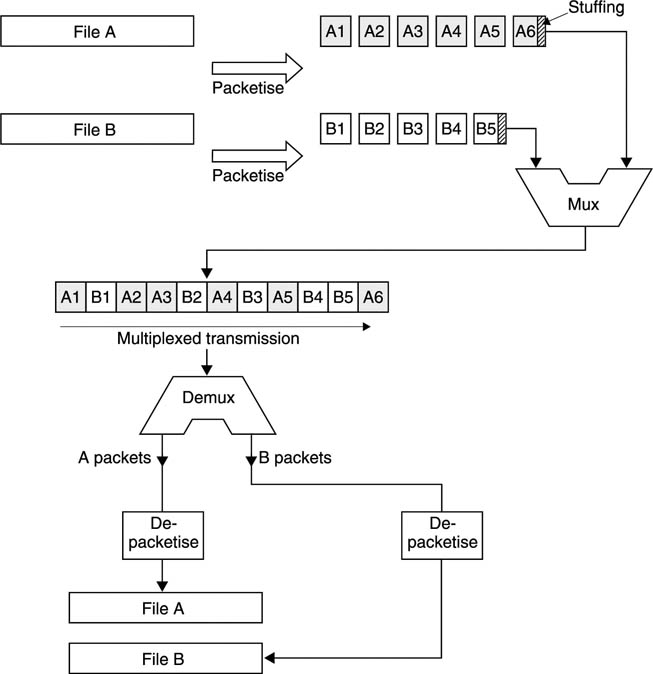
A central arbitrator is relatively simple to implement because when all decisions are taken centrally there can be no timing difficulty (assuming a well-engineered system). In a distributed system, there is an extra difficulty due to the finite time taken for signals to travel down the data paths between nodes.

Figure 9.51 shows the structure of Ethernet which uses a protocol called CSMA/CD (carrier sense multiple access with collision detect) developed by DEC and Xerox. This is a distributed arbitration network where each node follows some simple rules. The first of these is not to transmit if an existing bus signal is detected. The second is not to transmit more than a certain quantity of data before releasing the bus. Devices wanting to use the bus will see bus signals and so will wait until the present bus transaction finishes. This must happen at some point because of the frame size limit. When the frame is completed, signalling on the bus should cease. The first device to sense the bus becoming free and to assert its own signal will prevent any other nodes transmitting according to the first rule. Where numerous devices are present it is possible to give them a priority structure by providing a delay between sensing the bus coming free and beginning a transaction. High-priority devices will have a short delay so they get in first. Lower-priority devices will only be able to start a transaction if the high-priority devices don’t need to transfer.

Figure 9.51 In Ethernet collisions can occur because of the finite speed of the signals. A ‘back-off’ algorithm handles collisions, but they do reduce the network throughput.

It might be thought that these rules would be enough and everything would be fine. Unfortunately the finite signal speed means that there is a flaw in the system. Figure 9.51 shows why. Device A is transmitting and devices B and C both want to transmit and have equal priority. At the end of A’s transaction, devices B and C see the bus become free at the same instant and start a transaction. With two devices driving the bus, the resultant waveform is meaningless. This is known as a collision and all nodes must have means to recover from it. First, each node will read the bus signal at all times. When a node drives the bus, it will also read back the bus signal and compare it with what was sent. Clearly if the two are the same all is well, but if there is a difference, this must be because a collision has occurred and two devices are trying to determine the bus voltage at once.

If a collision is detected, both colliding devices will sense the disparity between the transmitted and readback signals, and both will release the bus to terminate the collision. However, there is no point is adhering to the simple protocol to reconnect because this will simply result in another collision. Instead each device has a built-in delay which must expire before another attempt is made to transmit. This delay is not fixed, but is controlled by a random number generator and so changes from transaction to transaction.

The probability of two node devices arriving at the same delay is infinitesimally small. Consequently if a collision does occur, both devices will drop the bus, and they will start their back-off timers. When the first timer expires, that device will transmit and the other will see the transmission and remain silent. In this way the collision is not only handled, but prevented from happening again.

The performance of Ethernet is usually specified in terms of the bit rate at which the cabling runs. However, this rate is academic because it is not available all the time. In a real network bit rate is lost by the need to send headers and error-correction codes and by the loss of time due to interframe spaces and collision handling. As the demand goes up, the number of collisions increases and throughput goes down. Collision-based arbitrators do not handle congestion well.

An alternative method of arbitration developed by IBM is show in Figure 9.52. This is known as a token ring system. All the nodes have an input and an output and are connected in a ring which must be complete for the system to work. Data circulate in one direction only. If data are not addressed to a node which receives them, the data will be passed on. When the data arrive at the addressed node, that node will capture the data as well as passing them on with an acknowledge added. Thus the data packet travels right around the ring back to the sending node. When the sending node receives the acknowledge, it will transmit a token packet. This token packet passes to the next node, which will pass it on if it does not wish to transmit. If no device wishes to transmit, the token will circulate endlessly. However, if a device has data to send, it simply waits until the token arrives again and captures it. This node can now transmit data in the knowledge that there cannot be a collision because no other node has the token.

Figure 9.52 In a token ring system only the node in possession of the token can transmit so collisions are impossible. In very large rings the token circulation time causes loss of throughput.

In simple token ring systems, the transmitting node transmits idle characters after the data packet has been sent in order to maintain synchronization. The idle character transmission will continue until the acknowledge arrives. In the case of long packets the acknowledge will arrive before the packet has all been sent and no idle characters are necessary. However, with short packets idle characters will be generated. These idle characters use up ring bandwidth.

Later token ring systems use early token release (ETR). After the packet has been transmitted, the sending node sends a token straight away. Another node wishing to transmit can do so as soon as the current packet has passed.

It might be thought that the nodes on the ring would transmit in their physical order, but this is not the case because a priority system exists. Each node can have a different priority if necessary. If a high-priority node wishes to transmit, as a packet from elsewhere passes through that node, the node will set reservation bits with its own priority level. When the sending node finishes and tranmits a token, it will copy that priority level into the token. In this way nodes with a lower priority level will pass the token on instead of capturing it. The token will ultimately arrive at the high-priority node.

The token ring system has the advantage that it does not waste throughput with collisions and so the full capacity is always available. However, if the ring is broken the entire network fails.

In Ethernet the performance is degraded by the number of transactions, not the number of nodes, whereas in token ring the performance is degraded by the number of nodes.

9.19 FireWire

FireWire9 is actually an Apple Computers Inc. trade name for the interface which is formally known as IEEE 1394–1995. It was originally intended as a digital audio network, but grew out of recognition. FireWire is more than just an interface as it can be used to form networks and if used with a computer effectively extends the computer’s data bus. Figure 9.53 shows that devices are simply connected together as any combination of daisy-chain or star network.

Figure 9.53 FireWire supports radial (star) or daisy-chain connection. Two-port devices pass on signals destined for a more distant device – they can do this even when powered down.

Any pair of devices can communicate in either direction, and arbitration ensures that only one device transmits at once. Intermediate devices simply pass on transmissions. This can continue even if the intermediate device is powered down as the FireWire carries power to keep repeater functions active.

Communications are divided into cycles which have a period of 125 μs. During a cycle, there are 64 time slots. During each time slot, any one node can communicate with any other, but in the next slot, a different pair of nodes may communicate. Thus FireWire is best described as a time-division multiplexed (TDM) system. There will be a new arbitration between the nodes for each cycle.

FireWire is eminently suitable for video/computer convergent applications because it can simultaneously support asynchronous transfers of non-real-time computer data and isochronous transfers of real-time audio/video data. It can do this because the arbitration process allocates a fixed proportion of slots for isochronous data (about 80 per cent) and these have a higher priority in the arbitration than the asynchronous data. The higher the data rate a given node needs, the more time slots it will be allocated. Thus a given bit rate can be guaranteed throughout a transaction; an prerequisite of real-time A/V data transfer.

It is the sophistication of the arbitration system which makes FireWire remarkable. Some of the arbitration is in hardware at each node, but some is in software which only needs to be at one node. The full functionality requires a computer somewhere in the system which runs the isochronous bus management arbitration. Without this only asynchronous transfers are possible. It is possible to add or remove devices whilst the system is working. When a device is added the system will recognize it through a periodic learning process. Essentially every node on the system transmits in turn so that the structure becomes clear.

The electrical interface of FireWire is shown in Figure 9.54. It consists of two twisted pairs for signalling and a pair of power conductors. The twisted pairs carry differential signals of about 220 mV swinging around a common mode voltage of about 1.9 V with an impedance of 112W. Figure 9.55 shows how the data are transmitted. The host data are simply serialized and used to modulate twisted pair A. The other twisted pair (B) carries a signal called strobe, which is the exclusive-OR of the data and the clock. Thus whenever a run of identical bits results in no transitions in the data, the strobe signal will carry transitions. At the receiver another exclusive-OR gate adds data and strobe to recreate the clock.

Figure 9.54 FireWire uses twin twisted pairs and a power pair.

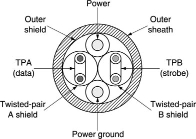
Figure 9.55 The strobe signal is the X-OR of the data and the bit clock. The data and strobe signals together form a self-clocking system.

This signalling technique is subject to skew between the two twisted pairs and this limits cable lengths to about 10 metres between nodes. Thus FireWire is not a long-distance interface technique, instead it is very useful for interconnecting a large number of devices in close proximity. Using a copper interconnect, FireWire can run at 100, 200 or 400 Mbits/s, depending on the specific hardware. It is proposed to create an optical fibre version which would run at gigabit speeds.

9.20 Broadband networks and ATM

Broadband ISDN (B-ISDN) is the successor to N-ISDN and in addition to offering more bandwidth, offers practical solutions to the delivery of any conceivable type of data. The flexibility with which ATM operates means that intermittent or one-off data transactions which only require asynchronous delivery can take place alongside isochronous MPEG video delivery. This is known as application independence whereby the sophistication of isochronous delivery does not raise the cost of asynchronous data. In this way, generic data, video, speech and combinations of the above can co-exist.

ATM is multiplexed, but it is not time-division multiplexed. TDM is inefficient because if a transaction does not fill its allotted bandwidth, the capacity is wasted. ATM does not offer fixed blocks of bandwidth, but allows infinitely variable bandwidth to each transaction. This is done by converting all host data into small fixed-size cells at the adaptation layer. The greater the bandwidth needed by a transaction, the more cells per second are allocated to that transaction. This approach is superior to the fixed bandwidth approach, because if the bit rate of a particular transaction falls, the cells released can be used for other transactions so that the full bandwidth is always available.

As all cells are identical in size, a multiplexer can assemble cells from many transactions in an arbitrary order. The exact order is determined by the quality of service required, where the time positioning of isochronous data would be determined first, with asynchronous data filling the gaps.

Figure 9.56 shows how a broadband system might be implemented. The transport network would typically be optical fibre based, using SONET (synchronous optical network) or SDH (synchronous digital hierarchy). These standards differ in minor respects. Figure 9.57 shows the bit rates available in each. Lower bit rates will be used in the access networks which will use different technology such as xDSL.

Figure 9.56 Structure and terminology of a broadband network. See text.

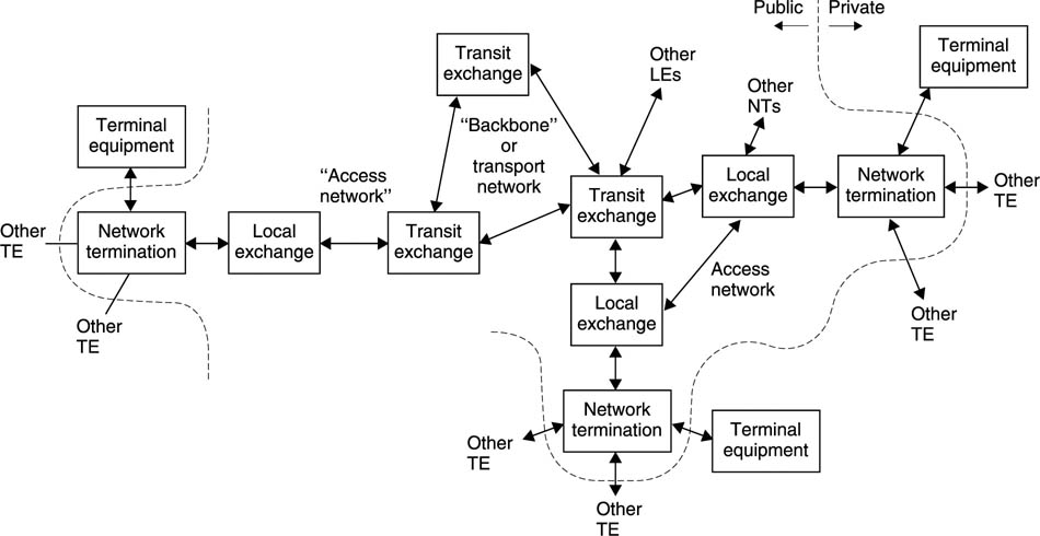
Figure 9.57 Bit rates available in SONET and SDH.

SONET and SDH assemble ATM cells into a structure known as a container in the interests of efficiency. Containers are passed intact between exchanges in the transport network. The cells in a container need not belong to the same transaction, they simply need to be going the same way for at least one transport network leg.

The cell-routing mechanism of ATM is unusual and deserves explanation. In conventional networks, a packet must carry the complete destination address so that at every exchange it can be routed closer to its destination. The exact route by which the packet travels cannot be anticipated and successive packets in the same transaction may take different routes. This is known as a connectionless protocol.

In contrast, ATM is a connection oriented protocol. Before data can be transferred, the network must set up an end-to-end route. Once this is done, the ATM cells do not need to carry a complete destination address. Instead they only need to carry enough addressing so that an exchange or switch can distinguish between all the expected transactions.

The end-to-end route is known as a virtual channel which consists of a series of virtual links between switches. The term ‘virtual channel’ is used because the system acts like a dedicated channel even though physically it is not. When the transaction is completed the route can be dismantled so that the bandwidth is freed for other users. In some cases, such as delivery of a TV station’s output to a transmitter, or as a replacement for analog cable TV the route can be set up continuously to form what is known as a permanent virtual channel.

The addressing in the cells ensures that all cells with the same address take the same path, but owing to the multiplexed nature of ATM, at other times and with other cells a completely different routing scheme may exist. Thus the routing structure for a particular transaction always passes cells by the same route, but the next cell may belong to another transaction and will have a different address causing it to routed in another way.

The addressing structure is hierarchical. Figure 9.58(a) shows the ATM cell and its header. The cell address is divided into two fields, the virtual channel identifier and the virtual path identifier. Virtual paths are logical groups of virtual channels which happen to be going the same way. An example would be the output of a video-on-demand server travelling to the first switch. The virtual path concept is useful because all cells in the same virtual path can share the same container in a transport network. A virtual path switch shown in Figure 9.58(b) can operate at the container level whereas a virtual channel switch (c) would need to dismantle and reassemble containers.

Figure 9.58 The ATM cell (a) carries routing information in the header. ATM paths carrying a group of channels can be switched in a virtual path switch (b). Individual channel switching requires a virtual channel switch which is more complex and causes more delay.

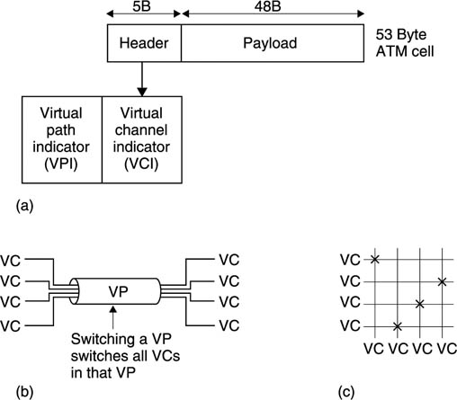
When a route is set up, at each switch a table is created. When a cell is received at a switch the VPI and/or VCI code is looked up in the table and used for two purposes. First, the configuration of the switch is obtained, so that this switch will correctly route the cell, second, the VPI and/or VCI codes may be updated so that they correctly control the next switch. This process repeats until the cell arrives at its destination.

In order to set up a path, the initiating device will initially send cells containing an ATM destination address, the bandwidth and quality of service required. The first switch will reply with a message containing the VPI/VCI codes which are to be used for this channel. The message from the initiator will propagate to the destination, creating look-up tables in each switch. At each switch the logic will add the requested bandwidth to the existing bandwidth in use to check that the requested quality of service can be met. If this succeeds for the whole channel, the destination will reply with a connect message which propagates back to the initiating device as confirmation that the channel has been set up. The connect message contains an unique call reference value which identifies this transaction. This is necessary because an initiator such a file server may be initiating many channels and the connect messages will not necessarily return in the same order as the set-up messages were sent.

The last switch will confirm receipt of the connect message to the destination and the initiating device will confirm receipt of the connect message to the first switch.

ATM works by dividing all real data messages into cells of 48 bytes each. At the receiving end, the original message must be recreated. This can take many forms. Figure 9.59 shows some possibilities. The message may be a generic data file having no implied timing structure. The message may be a serial bitstream with a fixed clock frequency, known as UDT (unstructured data transfer). It may be a burst of data bytes from a TDM system.

Figure 9.59 Types of data which may need adapting to ATM.

The application layer in ATM has two sub-layers shown in Figure 9.60. The first is the segmentation and reassembly (SAR) sublayer which must divide the message into cells and rebuild it to get the binary data right. The second is the convergence sublayer (CS) which recovers the timing structure of the original message. It is this feature which makes ATM so appropriate for delivery of audio/visual material. Conventional networks such as the Internet don’t have this ability.

Figure 9.60 ATM adaption layer has two sublayers, segmentation and convergence.

In order to deliver a particular quality of service, the adaptation layer and the ATM layer work together. Effectively the adaptation layer will place constraints on the ATM layer, such as cell delay, and the ATM layer will meet those constraints without needing to know why. Provided the constraints are met, the adaptation layer can rebuild the message. The variety of message types and timing constraints leads to the adaptation layer having a variety of forms.

The adaptation layers which are most relevant to MPEG applications are AAL-1 and AAL-5. AAL-1 is suitable for transmitting MPEG-2 multi-program transport streams at constant bit rate and is standardized for this purpose in ETS 300814 for DVB application. AAL-1 has an integral forward error correction (FEC) scheme. AAL-5 is optimized for single-program transport streams (SPTS) at a variable bit rate and has no FEC.

AAL-1 takes as an input the 188-byte transport stream packets which are created by a standard MPEG-2 multiplexer. The transport stream bit rate must be constant but it does not matter if statistical multiplexing has been used within the transport stream.

The Reed–Solomon FEC of AAL-1 uses a codeword of size 128 so that the codewords consist of 124 bytes of data and 4 bytes of redundancy, making 128 bytes in all. Thirty-one 188-byte TS packets are restructured into this format. The 256-byte codewords are then subject to a block interleave. Figure 9.61 shows that 47 such codewords are assembled in rows in RAM and then columns are read out. These columns are 47 bytes long and, with the addition of an AAL header byte make up a 48-byte ATM packet payload. In this way the interleave block is transmitted in 128 ATM cells.

Figure 9.61 The interleave structure used in AAL-1.

The result of the FEC and interleave is that the loss of up to four cells in 128 can be corrected, or a random error of up to two bytes can be corrected in each cell. This FEC system allows most errors in the ATM layer to be corrected so that no retransmissions are needed. This is important for isochronous operation.

The AAL header has a number of functions. One of these is to identify the first ATM cell in the interleave block of 128 cells. Another function is to run a modulo-8 cell counter to detect missing or out-of sequence ATM cells. If a cell simply fails to arrive, the sequence jump can be detected and used to flag the FEC system so that it can correct the missing cell by erasure (see section 6.22). In a manner similar to the use of program clock reference (PCR) in MPEG, AAL-1 embeds a timing code in ATM cell headers. This is called the synchronous residual time stamp (SRTS) and in conjunction with the ATM network clock allows the receiving AAL device to reconstruct the original data bit rate. This is important because in MPEG applications it prevents the PCR jitter specification being exceeded.

In AAL-5 there is no error correction and the adaptation layer simply reformats MPEG TS blocks into ATM cells. Figure 9.62 shows one way in which this can be done. Two TS blocks of 188 bytes are associated with an 8-byte trailer known as CPCS (common part convergence sublayer). The presence of the trailer makes a total of 384 bytes which can be carried in eight ATM cells. AAL-5 does not offer constant delay and external buffering will be required, controlled by reading the MPEG PCRs in order to reconstruct the original time axis.

Figure 9.62 The AAL-5 adaptation layer can pack MPEG transport packets in this way.

References

1.SMPTE 259M – 10-bit 4:2:2 Component and 4FSc NTSC Composite Digital Signals – Serial Digital Interface

2.2.Eguchi, T., Pathological check codes for serial digital interface systems. Presented at SMPTE Conference, Los Angeles, October 1991

3.SMPTE 305M Serial – Data Transport Interface

4.Audio Engineering Society, AES recommended practice for digital audio engineering – serial transmission format for linearly represented digital audio data. J. Audio Eng. Soc., 33, 975–984 (1985)

5.EIA RS-422A. Electronic Industries Association, 2001 Eye Street NW, Washington, DC 20006, USA

6.Smart, D.L., Transmission performance of digital audio serial interface on audio tie lines. BBC Designs Dept Technical Memorandum, 3.296/84

7.European Broadcasting Union, Specification of the digital audio interface. EBU Doc. Tech., 3250

8.Rorden, B. and Graham, M., A proposal for integrating digital audio distribution into TV production. J. SMPTE, 606–608 (September, 1992)

9.Wicklegren, I.J., The facts about FireWire. IEEE Spectrum, 19–25 (1997)