In this chapter, we provide a general description of SQL, give the background and history of SQL, and discuss several applications areas of the language. We also cover basic subjects, such as the database and database server. SQL is based on the theory of the relational model. To use SQL, some knowledge of this model is invaluable. Therefore, in Section 1.3, we describe the relational model. In Section 1.4, we briefly describe what SQL is, what can be done with the language, and how it differs from other languages (such as Java, Visual Basic, or Pascal). Section 1.6 is devoted to the history of SQL. Although SQL is thought of as a very modern language, it has a history dating back to 1972. SQL has been implemented in many products and has a monopoly position in the world of database languages. In Section 1.9 we outline the most important current standards for SQL, and in Section 1.10, we give a brief outline of the most important SQL products.

This first chapter closes with a description of the structure of the book. Each chapter is summarized in a few sentences.

Structured Query Language (SQL) is a database language used for formulating statements that are processed by a database server. This sentence contains three important concepts: database, database server, and database language. We begin with an explanation of each of these terms.

What is a database? In this book, we use a definition that is derived from Chris J. Date’s definition; see [Date 95]:

Card index files do not, therefore, constitute a database. On the other hand, the large files of banks, insurance companies, telephone companies, or the state transport department can be considered databases. These databases contain data about addresses, account balances, car registration plates, weights of vehicles, and so on. For example, the company you work for probably has its own computers, and these are used to store salary-related data.

Data in a database becomes useful only if something is done with it. According to the definition, data in the database is managed by a separate programming system. We call this system a database server or database-management system (DBMS). MySQL is such a database server. A database server enables users to process data stored in a database. Without a database server, it is impossible to look at data, or to update or delete obsolete data, in the database. The database server alone knows where and how data is stored. A definition of a database server is given in [ELMA03] by R. Elmasri:

A database server never changes or deletes the data in a database by itself. Someone or something has to give the command for this to happen. Examples of commands that a user could give to the database server are “delete all data about the vehicle with the registration plate number DR-12-DP” or “give the names of all the companies that haven’t paid the invoices of last March.” However, users cannot communicate with the database server directly. Commands are given to a database server with the help of an application. An application is always between the user and the database server. Section 1.4 discusses this subject.

The definition of the term database also contains the word persistent. This means that data in a database remains there permanently, until it is changed or deleted explicitly. If you store new data in a database and the database server sends the message back that the storage operation was successful, you can be sure that the data will still be there tomorrow (even if you switch off your computer). This is unlike the data that we store in the internal memory of a computer. If the computer is switched off, that data is lost forever; it is, therefore, not persistent.

Commands are given to a database server with the help of special languages called database languages. Commands, also known as statements, which are formulated according to the rules of the database language, are entered by users using special software and are processed by the database server. Every database server, from whichever manufacturer, possesses a database language. Some systems support more than one. All these languages are different, which makes it possible to divide them into groups. The relational database languages form one of these groups. An example of such a language is SQL.

How does a database server store data in a database? A database server uses neither a chest of drawers nor a filing cabinet to hold information; instead, computers work with storage media such as tapes, floppy disks, and magnetic and optical disks. The manner in which a database server stores information on these media is very complex and technical, and it is not explained in detail in this book. In fact, it is not required to have this technical knowledge because one of the most important tasks of a database server is to offer data independence. This means that users do not need to know how or where data is stored: To users, a database is simply a large reservoir of information. Storage methods are also completely independent of the database language being used. In a way, this resembles the process of checking luggage at an airport. It is none of our business where and how the airline stores our luggage; the only thing we are interested in is whether the luggage is at our destination upon arrival.

Another important task of a database server is to maintain the integrity of the data stored in a database. This means, first, that the database server has to make sure that database data always satisfies the rules that apply in the real world. Consider, for example, the case of an employee who is allowed to work for one department only. It should never be possible, in a database managed by a database server, for that particular employee to be registered as working for two or more departments. Second, integrity means that two different pieces of database data do not contradict one another. This is also known as data consistency. (As an example, in one place in a database, Mr. Johnson might be recorded as being born on August 4, 1964, and in another place he might be given a birth date of December 14, 1946. These two pieces of data are obviously inconsistent.) Each database server is designed to recognize statements that can be used to specify constraints. After these rules are entered, the database server takes care of their implementation.

SQL is based on a formal and mathematical theory. This theory, which consists of a set of concepts and definitions, is called the relational model. The relational model was defined by E. F. Codd in 1970, when he was employed by IBM. He introduced the relational model in the almost legendary article entitled “A Relational Model of Data for Large Shared Data Banks”; see [CODD70]. This relational model provides a theoretical basis for database languages. It consists of a small number of simple concepts for recording data in a database, together with a number of operators to manipulate the data. These concepts and operators are principally borrowed from set theory and predicate logic. Later, in 1979, Codd presented his ideas for an improved version of the model; see [CODD79] and [CODD90].

The relational model has served as an example for the development of various database languages, including QUEL (see [STON86]), SQUARE (see [BOYC73a]), and, of course, SQL. These database languages are based on the concepts and ideas of that relational model and are therefore called relational database languages; SQL is an example. The rest of this part concentrates on the following terms used in the relational model, which appear extensively in this book:

Please note that this is not a complete list of all the terms used by the relational model. Most of these terms are discussed in detail in Part III, “Creating Database Objects.” For more extensive descriptions, see [CODD90] and [DATE95].

Table, Column, and Row

Data can be stored in a relational database in only one format, and that is in tables. The official name for a table is actually relation, and the term relational model stems from this name. We have chosen to use the term table because that is the word used in SQL.

Informally, a table is a set of rows, with each row consisting of a set of values. All the rows in a certain table have the same number of values. Figure 1.1 shows an example of a table called the PLAYERS table. This table contains data about five players who are members of a tennis club.

Figure 1.1. The concepts value, row, column, and table

This PLAYERS table has five rows, one for each player. A row with values can be considered as a set of data elements that belong together. For example, in this table, the first row consists of the values 6, Parmenter, R, and Stratford. This information tells us that there is a player with number 6, that his last name is Parmenter and his initial is R, and that he lives in the town Stratford.

PLAYERNO, NAME, INITIALS, and TOWN are the names of the columns in the table. The PLAYERNO column contains the values 6, 44, 83, 100, and 27. This set of values is also known as the population of the PLAYERNO column. Each row has a value for each column. Therefore, in the first row there is a value for the PLAYERNO column and a value for the NAME column, and so on.

A table has two special properties:

• The intersection of a row and a column can consist of only one value, an atomic value. An atomic value is an indivisible unit. The database server can deal with such a value only in its entirety.

• The rows in a table have no specific order. One should not think in terms of the first row, the last three rows, or the next row. The contents of a table should actually be considered a set of rows in the true sense of the word.

Constraints

In the first section of this chapter, we described the integrity of the data stored in tables, the database data. The contents of a table must satisfy certain rules, the so-called integrity constraints (integrity rules). Two examples of integrity constraints are: The player number of a player may not be negative, and two different players may not have the same player number. Integrity constraints can be compared to road signs. They also indicate what is allowed and what is not allowed.

Integrity constraints should be enforced by a relational database server. Each time a table is updated, the database server has to check whether the new data satisfies the relevant integrity constraints. This is a task of the database server. The integrity constraints must be specified first so that they are known to the database server.

Integrity constraints can have several forms. Because some are used so frequently, they have been assigned special names, such as primary key, candidate key, alternate key, and foreign key. The analogy with the road signs (as shown in Figure 1.2) applies here as well. Special symbols have been invented for road signs that are frequently used, and they also were given names, such as a right-of-way sign or a stop sign. We explain those named integrity constraints in the following sections.

Figure 1.2. Integrity constraints are the road signs of a database

Primary Key

The primary key of a table is a column (or a combination of columns) that is used as a unique identification of rows in that table. In other words, two different rows in a table may never have the same value in their primary key, and for every row in the table, the primary key must always have one value. The PLAYERNO column in the PLAYERS table is the primary key for this table. Two players, therefore, may never have the same number, and there may never be a player without a number.

We come across primary keys everywhere. For example, the table in which a bank stores data about bank accounts will have the column bank account number as primary key. And when we create a table in which different cars are registered, the license plate will be the primary key, as shown in Figure 1.3.

Figure 1.3. License plate as possible primary key

Foreign Key

A foreign key is a column (or combination of columns) in a table in which the population is a subset of the population of the primary key of a table. (This does not have to be another table.) Foreign keys are sometimes called referential keys.

Imagine that, in addition to the PLAYERS table, there is a TEAMS table; see Figure 1.4. The TEAMNO column is called the primary key of this table. The PLAYERNO column in this table represents the captain of each particular team. This has to be an existing player number, one that is found in the PLAYERS table. The population of this column represents a subset of the population of the PLAYERNO column in the PLAYERS table. PLAYERNO in the TEAMS table is called a foreign key.

Figure 1.4. The foreign key

Now you can see that we can combine two tables. We do this by including the PLAYERNO column in the TEAMS table, thus establishing a link with the PLAYERNO column in the PLAYERS table.

As already stated, SQL is a relational database language. Among other things, the language consists of statements to insert, update, delete, query, and protect data. The following is a list of statements that can be formulated with SQL:

SQL has already been implemented by many vendors as the database language for their database server. For example, IBM, MySQL, and Oracle are all vendors of SQL products. Thus, SQL is not the name of a certain product that has been brought onto the market by one particular vendor. Although SQL is not a database server, in this book, SQL is considered, for simplicity, to be a database server as well as a language. Of course, wherever necessary, a distinction is drawn.

We call SQL a relational database language because it is associated with data that has been defined according to the rules of the relational model. (However, we must note that on particular points, the theory and SQL differ; see [CODD90].) Because SQL is a relational database language, for a long time, it has been grouped with the declarative or nonprocedural database languages. By declarative and nonprocedural, we mean that users (with the help of statements) have to specify only which data elements they want, not how they must be accessed one by one. Well-known languages such as C, C++, Java, PHP, Pascal, and Visual Basic are examples of procedural languages.

Nowadays, however, SQL can no longer be called a pure declarative language. Since the early 1990s, many vendors have added procedural extensions to SQL. These make it possible to create procedural database objects such as triggers and stored procedures; see Part V, “Procedural Database Objects.” Traditional statements such as IF-THEN-ELSE and WHILE-DO have also been added. Although most of the well-known SQL statements are still not procedural by nature, SQL has changed into a hybrid language consisting of procedural and nonprocedural statements. MySQL has also been extended with these procedural database objects.

SQL can be used in two ways. First, SQL can be used interactively: For example, a user enters an SQL statement on the spot and the database server processes it immediately. The result is also immediately visible. Interactive SQL is intended for application developers and for end users who want to create reports themselves.

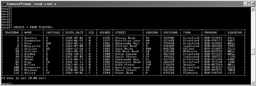
The products that support interactive SQL can be split in two groups: the somewhat old-fashioned products with a terminal-like interface and those with a modern graphical interface. MySQL includes a product with a terminal-like interface that bears the same name as the database server: MYSQL. Figure 1.5 shows what this program looks like. First an SQL statement is entered, and then the result is shown underneath.

Figure 1.5. An example of the query program called MYSQL that specifies the SQL statements interactively

However, products with a more graphical interface are also available for interactive use that are not from MySQL, such as WinSQL; see Figure 1.6.

Figure 1.6. An example of the query program WinSQL

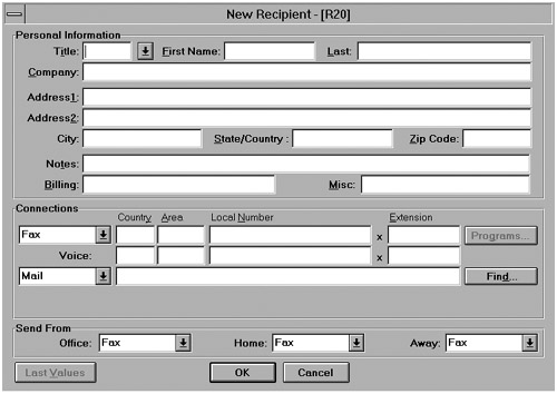
The second way in which SQL can be used is preprogrammed SQL. Here, the SQL statements are embedded in an application that is written in another programming language. Results from these statements are not immediately visible to the user but are processed by the enveloping application. Preprogrammed SQL appears mainly in applications developed for end users. These end users do not need to learn SQL to access the data, but they work from simple screens and menus designed for their applications. Examples are applications to record customer information and applications to handle stock management. Figure 1.7 contains an example of a screen with fields in which the user can enter the address without any knowledge of SQL. The application behind this screen has been programmed to pass certain SQL statements to the database server. The application, therefore, uses SQL statements to transfer the information that has been entered into the database.

Figure 1.7. SQL is shielded in many applications; users can see only the input fields

In the early stages of the development of SQL, there was only one method for preprogrammed SQL, called embedded SQL. In the 1990s, other methods appeared. The most important is called Call Level Interface SQL (CLI SQL). There are many variations of CLI SQL, such as Open Database Connectivity (ODBC) and Java Database Connectivity (JDBC). The most important ones are described in this book. The different methods of preprogrammed SQL are also called the binding styles.

The statements and features of interactive and preprogrammed SQL are virtually the same. By this, we mean that most statements that can be entered and processed interactively can also be included (embedded) in an SQL application. Preprogrammed SQL has been extended with a number of statements that are added only to make it possible to merge the SQL statements with the non-SQL statements. In this book, we are primarily engaged in interactive SQL. Preprogrammed SQL is dealt with in Part IV, “Programming with SQL.”

Three important components are involved in the interactive and preprogrammed processing of SQL statements: the user, the application, and the database server; see Figure 1.8. The database server is responsible for storing and accessing data on disk. The application and definitely the user have nothing to do with this. The database server processes the SQL statements that are delivered by the application. In a defined way, the application and the database server can send SQL statements between them. The result of an SQL statement is then returned to the user.

Figure 1.8. The user, the application, and the database server are pivotal for the processing of SQL

SQL is used in a wide range of applications. If SQL is used, it is important to know what kind of application is being developed. For example, does an application execute many simple SQL statements or just a few very complex ones? This can affect how SQL statements should be formulated in the most efficient way, which statements are selected, and how SQL is used. To simplify this discussion, we introduce a hierarchical classification of applications to which we refer, if relevant, in other chapters:

The first subdivision has to do with whether SQL statements are preprogrammed. This is not the case for products that support SQL interactively. The user determines, directly or indirectly, which SQL statements are created.

The preprogrammed applications are subdivided into input and reporting applications. The input applications have two variations: online and batch. An online input application, for example, can be written in Visual Basic and SQL and allows data to be added to a database. This type of application is typically used by many users concurrently, and the preprogrammed SQL statements are relatively simple. Batch input applications read files containing new data and add the data to an existing database. These applications usually run at regular times and require much processing. The SQL statements are again relatively simple.

A batch reporting application generates reports. For example, every Sunday, a report is generated that contains the total sales figures for every region. Every Monday morning, this report is delivered by internal mail to the desk of the manager or is sent to his e-mail address. Many companies use this kind of application. Usually, a batch reporting application contains only a few statements, but these are complex.

The market for applications in which users work interactively with SQL is less well organized. For the first subcategory, the query tools, users must have a knowledge of relational concepts. In the query process, the user works with, among other things, tables, columns, rows, primary keys, and foreign keys.

Within the category of query tools, we can identify three subcategories. In the first category, the users have to type in SQL statements directly. They must be fully acquainted with the grammar of SQL. WinSQL, which we already discussed, is such a program. Figure 1.6 shows what this program looks like. In the middle of the screen there is an SQL statement with the result underneath it.

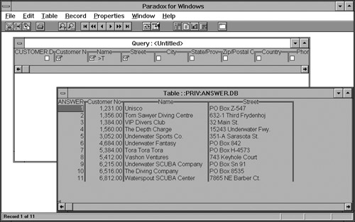
Query-By-Example (QBE) was designed in the 1970s by Moshé Zloof; see [ZLOO7]. QBE was intended to be a relational database language and, in some ways, to provide an alternative for SQL. Eventually, the language served as a model for an entire family of products, all of which had a comparable interface. It is not necessary for users of QBE to understand the syntax of SQL because SQL statements are automatically generated. Users simply draw tables and fill their conditions and specifications into those tables. QBE has been described as a graphical version of SQL. This is not completely true, but it gives an indication of what QBE is. Figure 1.9 shows what a QBE question looks like.

Figure 1.9. An example of Query-By-Example

Some vendors have tried to offer users the strength and flexibility of SQL without the necessity of learning the language. This is implemented by a natural language interface that is put on top of SQL, enabling users to define their questions in simple English sentences. Next, these sentences are translated into SQL. The market for this type of products has always been small, but it still is a very interesting category of query tools.

Again, to use these query tools, the user has to understand the principles of a relational database, and this can be too technical for some users. Nevertheless, experts in the field of marketing, logistics, or sales who have no technical background still will want to access the database data. For this purpose, the business intelligence tools have been designed. Here, a thick software layer is placed on top of SQL, meaning that neither SQL nor relational concepts are visible.

In this category, the statistical packages are probably the oldest. Products such as SAS and SPSS have been available for a long time. These tools offer their own languages for accessing data in databases and, of course, for performing statistical analysis. Generally, these are specialized and very powerful languages. Behind the scenes, their own statements are translated into SQL statements, if appropriate.

Very popular within the business intelligence tools is the category called OLAP tools. OLAP stands for online analytical processing, a term introduced by E. F. Codd. These are products designed for users who want to look at their sales, marketing, or production figures from different points of view and at different levels of detail.

Users of OLAP applications do not see the familiar relational interface, which means no “flat” tables or SQL, but work with a so-called multidimensional interface. Data is grouped logically within arrays, which consist of dimensions, such as region, product, and time. Within a dimension, hierarchies of elements can be built. The element Amsterdam belongs, for example, to the Netherlands, and the Netherlands belongs to Northern Europe. All three elements belong to the dimension called region. Unfortunately, all vendors have their own terminology. Cube, model, variable, and multidimensional table are all alternative names for array.

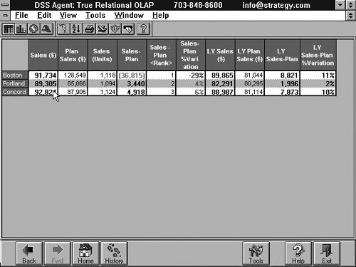
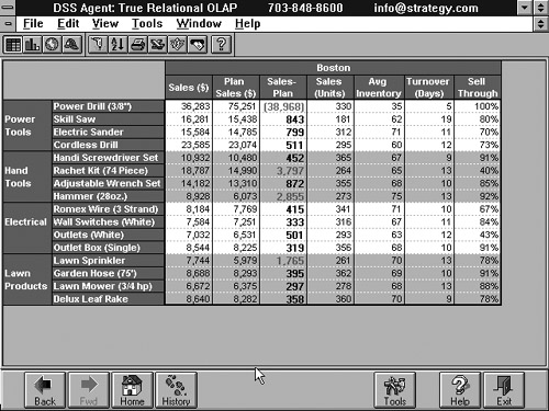
It falls outside the context of this book to give a detailed picture of OLAP, but to give you an idea of what is involved, we have included a simple example. Figure 1.10 contains a number of sales figures per region. There are three sales regions: Boston, Portland, and Concord. We can see that in the fourth column, the sales figure of Boston is given in brackets. This implies that this number is too low. This is correct because Boston was supposed to achieve $128,549 (see the second column in the table), but achieved only $91,734 (see the first column). This is clearly a long way behind the planned sales. Managers would probably like to know the reason for this and would like to see more detailed figures. To see these figures, all they have to do is click on the word Boston; the figures represented in Figure 1.11 then would be shown. Here, the sales figures in Boston are broken down per product. This result shows that not all the products are selling badly—only power drills. Of course, this is not the end of the story, and the user still does not know what is going on, but hopefully this simple example shows the power of OLAP. Without the need to learn SQL, the user can play with data, and that can be very useful. For a more detailed description of OLAP, see [THOM02].

Figure 1.10. Three sales regions with their respective sales figures

Figure 1.11. The sales figures of the sales region Boston, split into products

The last category of business intelligence tools is the data mining tools. Incorrectly, these tools are sometimes classified together with OLAP tools to stress that they have much in common. Whereas OLAP tools make it possible for users to simply look at data from different viewpoints and usually present data or summarized data stored in the database, data mining tools never present data or a total as a result. Their strength is to find trends and patterns in the data. For example, they can be used to try to find out whether certain products are bought together, what the dominant characteristics are of customers who take out life insurance policies, or what the characteristics are of a product that sells well in a big city. The technology used internally by this kind of tool is primarily based on artificial intelligence. Of course, these tools must also access data to discover trends; therefore, they use SQL. For an introduction to data mining, see [LARO04].

The complexity of the SQL statements generated by statistical, OLAP, and data mining tools can be quite high. This means that much work must be done by the database servers to process these statements.

Undoubtedly, many more categories of tools will appear in the future, but currently these are the dominant ones.

Finally, how tools or applications can locate the database server—or, in other words, how they exchange statements and results—is not discussed in detail in this book. In Part IV, we briefly touch on this topic. For now, you can assume that if an application wants to obtain information from a database server, a special piece of code must be linked with the application. This piece of code is called middleware and is (probably) developed by the database server vendor. Such code can be compared to a pilot who boards a ship to guide it into harbor.

The history of SQL is closely tied to the history of an IBM project called System R. The purpose of this project was to develop an experimental relational database server that bore the same name as the project: System R. This system was built in the IBM research laboratory in San Jose, California. The project was intended to demonstrate that the positive usability features of the relational model could be implemented in a system that satisfied the demands of a modern database server.

Figure 1.12. Don Chamberlin, one of the designers of SQL

A problem that had to be solved in the System R project was that there were no relational database languages. A language called Sequel was therefore developed as the database language for System R. The first articles about this language were written by the designers R. F. Boyce and D. D. Chamberlin; see [BOYC73a] and [CHAM76]. During the project, the language was renamed SQL because the name Sequel was in conflict with an existing trademark. (However, the language is still often pronounced as sequel.)

The System R project was carried out in three phases. In the first phase, Phase 0 (from 1974 to 1975), only a part of SQL was implemented. For example, the join (for linking data from various tables) was not implemented yet, and only a single-user version of the system was built. The purpose of this phase was to see whether implementation of such a system was possible. This phase ended successfully; see [ASTR80].

Phase 1 started in 1976. All the program code written for Phase 0 was put aside, and a new start was made. Phase 1 comprised the total system. This meant, among other things, that the multi-user capability and the join were incorporated. The development of Phase 1 took place between 1976 and 1977.

In the final phase, System R was evaluated. The system was installed at various places within IBM and with a large number of major IBM clients. The evaluation took place in 1978 and 1979. The results of this evaluation are described in [CHAM80], as well as in other publications. The System R project was finished in 1979.

The knowledge acquired and the technology developed in these three phases were used to build SQL/DS, which was the first IBM relational database server that was commercially available. In 1981, SQL/DS came onto the market for the operating system DOS/VSE, and in 1983, the VM/CMS version arrived. In that same year, DB2 was announced. Currently, DB2 is available for many operating systems.

IBM has published a great deal about the development of System R, which was happening at a time when relational database servers were being widely talked about at conferences and seminars. Therefore, it is not surprising that other companies also began to build relational systems. Some of them, such as Oracle, implemented SQL as the database language. In the last few years, many SQL products have appeared, and, as a result, SQL is now available for every possible system, large or small. Existing database servers have also been extended to include SQL support.

Toward the end of the 1980s, an SQL database server could be used in only one architecture: the monolithic architecture. In a monolithic architecture, everything runs on the same machine. This machine can be a large mainframe, a small PC, or a midrange computer with an operating system such as UNIX or Windows. Nowadays, there are many more architectures available, of which client/server and Internet are the very popular ones.

The monolithic architecture still exists; see Figure 1.13. With this architecture, the application and the database server run on the same machine. As explained in Section 1.4, the application passes SQL statements to the database server. The database server processes these statements, and the results are returned to the application. Finally, the results are shown to the users. Because both the application and the database server run on the same computer, communication is possible through very fast internal communication lines. In fact, we are dealing here with two processes that communicate internally.

Figure 1.13. The monolithic architecture

The arrival of cheaper and faster small computers in the 1990s led to the introduction of the client/server architecture. There are several subforms of this architecture, but we do not discuss them all here. It is important to realize that in a client/server architecture, the application runs on a different machine than the database server; see Figure 1.14. The machine on which the application runs is called the client machine; the other is the server machine. This is called working with a remote database. Internal communication usually takes place through a local area network (LAN) and occasionally through a wide area network (WAN). A user could start an application on his or her PC in Paris and retrieve data from a database located in Sydney. Communication would then probably take place through a satellite link.

Figure 1.14. The client/server architecture

The third architecture is the most recent one: the Internet architecture. The essence of this architecture is that the application running in a client/server architecture on the client machine is divided into two parts; see the left part of Figure 1.15. The part that deals with the user, or the user interface, runs on the client machine. The part that communicates with the database server, also called the application logic, runs on the server machine. In this book, these two parts are called, respectively, the client and the server application.

Figure 1.15. The Internet architecture

There are probably no SQL statements in the client application, but statements that call the server application. Languages such as HTML, JavaScript, and VBScript are often used for the client application. The call goes via the Internet or an intranet to the server machine, and the well-known Hypertext Transport Protocol (HTTP) is mostly used for this. The call comes in at a web server. The web server acts as a switchboard operator and knows which call has be sent to which server application.

Next, the call arrives at the server application. The server application sends the needed SQL statements to the database server. Many server applications run under the supervision of Java application servers, such as WebLogic from Bea Systems and Web-Sphere from IBM.

The results of the SQL statements are returned by the database server. In some way, the server application translates this SQL result to an HTML page and returns the page to the web server. And the web server knows, as switchboard operator, the client application to which the HTML answer must be returned

The right part of Figure 1.15 shows a variant of the Internet architecture in which the server application and the database server have also been placed on different server machines.

The fact that the database server and the database are remote is completely transparent to the programmer who is responsible for writing the application and the SQL statements. However, it is not irrelevant. With regard to language and efficiency aspects of SQL, it is important to know which architecture is used: monolithic, client/server, or Internet. In this book, we use the first one, but where relevant, we discuss the effect of client/server or Internet.

You can use data in a database for any kind of purpose. The first databases were mainly designed for the storage of operational data. We illustrate this with two examples. Banks, for example, keep record of all account holders, where they live, and what their balance is. In addition, for every transaction when it took place, the amount and the two account numbers involved are recorded. The bank statements that we receive periodically are probably reports (maybe generated with SQL) of these kinds of transactions. Airline companies have also developed databases that, through the years, have been filled with enormous amounts of operational data. They collect, for example, information about which passenger flew on which flight to which location.

Databases with operational data are developed to record data that is produced at production processes. Such data can be used, for example, to report on and monitor the progress of production processes and possibly to improve them or speed them up. Imagine if all the transactions at the bank were still processed by hand and your account information still kept in one large book. How long would it take for your transaction to be processed? Given the current size of banks, this would no longer be possible. Databases have become indispensable.

We call databases that are principally designed and implemented to store operational data transaction, operational, or production databases. Correspondingly, the matching applications are called transaction, operational, or production applications.

After some time, we started to use databases for other purposes. More data was used to produce reports. For example, how many passengers did we carry from London to Paris during the past few months? Or show the number of products sold per region for this year. Users receive these reports, for example, every Monday morning, either as hard copy on their desk or by e-mail. You will notice in this book that SQL offers many possibilities for creating reports. At first, these reports were created periodically and at times when the processing of the transaction programs was not disturbed, such as on Sunday or in the middle of the night.

More recently, as a result of the arrival of the PC, the requirements of users have increased. First, the demand for online reports increased. Online reports are produced the moment the user asks for it. Second, the need arose for users to create new reports themselves. To minimize the interruption of the transaction databases as much as possible, sepaate databases were built for that purpose. These databases are filled periodically with data stored in transaction databases and are primarily used for online reports. This type of database is called a data warehouse.

Bill Inmon defines a data warehouse as follows (see also [GILL96]):

This definition holds four important concepts. By subject oriented, we mean, for example, that all the customer information is stored together and that product information is stored together. The opposite of this is application oriented, in which a database contains data that is relevant for a certain application. Customer information can then be stored in two or more databases. This complicates reporting because data for a particular report has to be retrieved from multiple databases.

Briefly, the term integrated indicates a consistent encoding of data so that it can be retrieved and combined in an integrated fashion.

A data warehouse is a nonvolatile database. When a database is primarily used to generate reports, users definitely do not like it when the contents change constantly. Imagine that two users have to attend a meeting, and, to prepare for this, they both need to query the database to get the sales records for a particular region. Imagine that there are 10 minutes between these two queries. Within those 10 minutes, the database might have changed. At the meeting, the users will come up with different data. To prevent this, a data warehouse is updated periodically, not continuously. New data elements are added each evening or during the weekend.

The time variance of a data warehouse is another important aspect. Normally, we try to keep transaction databases as small as possible because the smaller the database, the faster the SQL processing speed. A common way to keep databases small is to delete the old data. The old data can be stored on magnetic tape or optical disk for future use. However, users of data warehouses expect to access historical data. They want to find out, for example, whether the total number of boat tickets to London has changed in the last ten years. Alternatively, they would like to know in what way the weather affects the sales of beer, and for that purpose they want to use the data of the last five years. This means that huge amounts of historical data must be included and that almost all the information is time variant. Therefore, a data warehouse of 1 TB or more in size is not unusual.

Note that when you design a database, you have to determine in advance how it will be used: Will it be a transaction database or a data warehouse? In this book, we make this distinction wherever relevant.

As mentioned before, each SQL database server has its own dialect. All these dialects resemble each other, but they are not completely identical. They differ in the statements they support, or some products contain more SQL statements than the others; the possibilities of statements can vary as well. Sometimes, two products support the same statement, but then the result of that statement varies from one product to another.

To avoid differences between the many database servers from several vendors, it was decided early that a standard for SQL had to be defined. The idea was that when the database servers would grow too much apart, acceptance by SQL market would diminish. A standard would ensure that an application with SQL statements would be easier to transfer from one database server to another.

In 1983, the International Organization for Standardization (ISO) and the American National Standards Institute (ANSI) started work on the development of an SQL standard. The ISO is the leading internationally oriented normalization and standardization organization, having as its objectives the promotion of international, regional, and national normalization. Many countries have local representatives of the ISO. The ANSI is the American branch of the ISO.

After many meetings and several false starts, the first ANSI edition of the SQL standard appeared in 1986. This is described in the document ANSI X3.135-1986, “Database Language SQL.” This SQL-86 standard is unofficially called SQL1. One year later, the ISO edition, called ISO 9075-1987, “Database Language SQL,” was completed; see [ISO87]. This report was developed under the auspices of Technical Committee TC97. The area of activity of TC97 is described as Computing and Information Processing. Its Subcommittee SC21 caused the standard to be developed. This means that the standards of ISO and ANSI for SQL1 or SQL-86 are identical.

SQL1 consists of two levels. Level 2 comprises the complete document, and Level 1 is a subset of Level 2. This implies that not all specifications of SQL1 belong to Level 1. If a vendor claims that its database server complies with the standard, the supporting level must be stated as well. This is done to improve the support and adoption of SQL1. It means that vendors can support the standard in two phases, first Level 1 and then Level 2.

The SQL1 standard is very moderate with respect to integrity. For this reason, it was extended in 1989 by including, among other things, the concepts of primary and foreign keys. This version of the SQL standard is called SQL89. The companion ISO document is called, appropriately, ISO 9075:1989, “Database Language SQL with Integrity Enhancements.” The ANSI version was completed simultaneously.

Immediately after the completion of SQL1 in 1987, a start was made on the development of a new SQL standard; see [ISO92]. This planned successor to SQL89 was called SQL2. This simple name was given because the date of publication was not known at the start. In fact, SQL89 and SQL2 were developed simultaneously. Finally, the successor was published in 1992 and replaced the current standard at that time (SQL89). The new SQL92 standard is an expansion of the SQL1 standard. Many new statements and extensions to existing statements have been added. For a complete description of SQL92, see [DATE97].

Just like SQL1, SQL92 has levels. The levels have names instead of numbers: entry, intermediate, and full. Full SQL is the complete standard. Intermediate SQL is, as far as functionality goes, a subset of full SQL, and entry SQL is a subset of intermediate SQL. Entry SQL can roughly be compared to SQL1 Level 2, although with some specifications extended. All the levels together can be seen as the rings of an onion; see Figure 1.16. A ring represents a certain amount of functionality. The bigger the ring, the more functionality is defined within that level. When a ring falls within the other ring, it means that it defines a subset of functionality.

Figure 1.16. The various levels of SQL1 and SQL92 represented as rings

At the time of this writing, many available products support entry SQL92. Some even claim to support intermediate SQL92, but not one product supports full SQL92. Hopefully, the support of the SQL92 levels will improve in the coming years.

Since the publication of SQL92, several additional documents have been added that extend the capabilities of the language. In 1995, SQL/CLI (Call Level Interface) was published. Later the name was changed to CLI95. There is more about CLI95 at the end of this section. The following year, SQL/PSM (Persistent Stored Modules), or PSM-96, appeared. The most recent addition, PSM96, describes functionality for creating so-called stored procedures. We deal with this concept extensively in Chapter 30, “Stored Procedures.” Two years after PSM96, SQL/OLB (Object Language Bindings), or OLB-98, was published. This document describes how SQL statements had to be included within the programming language Java.

Even before the completion of SQL92, a start was made on the development of its successor: SQL3. In 1999, the standard was published and bore the name SQL:1999. To be more in line with the names of other ISO standards, the small line that was used in the names of the previous editions was replaced by a colon. And because of the problems in 2000, it was decided that 1999 would not be shortened to 99. See [GULU99], [MELT01], and [MELT03] for more detailed descriptions of this standard.

When SQL:1999 was completed, it consisted of five parts: SQL/Framework, SQL/Foundation, SQL/CLI, SQL/PSM, and SQL/Bindings. SQL/OLAP, SQL/MED (Management of External Data), SQL/OLB, SQL/Schemata, and SQL/JRT (Routines and Types using the Java Programming Language) and SQL/XML(XML-Related Specifications) were added later, among other things. Thus, the current SQL standard of ISO consists of a series of documents. They all begin with the ISO code 9075. For example, the complete designation of the SQL/Framework is ISO/IEC 9075-1:2003.

Besides the 9075 documents, another group of documents focuses on SQL. The term used for this group is usually SQL/MM, short for SQL Multimedia and Application Packages. All these documents bear the ISO code 13249. SQL/MM consists of five parts. SQL/MM Part 1 is the SQL/MM Framework, Part 2 focuses on text retrieval (working with text), Part 3 is dedicated to spatial applications, Part 4 to still images (such as photos), and Part 5 to data mining (looking for trends and patterns in data).

In 2003, a new edition of SQL/Foundation appeared, along with new editions of some other documents, such as SQL/JRT and SQL/Schemata. At this moment, this group of documents can be seen as the most recent version of the international SQL standard. We refer to it by the abbreviation SQL:2003.

There were other organizations working on the standardization of SQL, such as The Open Group (then called the X/Open Group) and the SQL Access Group. The first does not get much attention any longer, so we do not discuss it in this book.

In July 1989, a number of mainly American vendors of SQL database servers, among them Informix, Ingres, and Oracle, set up a committee called the SQL Access Group. The objective of the SQL Access Group is to define standards for the interoperability of SQL applications. This means that SQL applications developed using those specifications are portable between the database servers of the associated vendors, and that a number of different database servers can be simultaneously accessed by these applications. At the end of 1990, the first report of the SQL Access Group was published and defined the syntax of a so-called SQL application interface. The first demonstrations in this field were given in 1991. Eventually, the ISO adopted the resulting document, and it was published under the name SQL/CLI. This document was mentioned earlier.

The most important technology that is derived from the work of the Open SQL Access Group—and, therefore, from SQL/CLI—is ODBC (Open Database Connectivity) from Microsoft. Because ODBC plays a very prominent role when accessing databases and is completely focused on SQL, we have devoted Chapter 28, “Introduction to ODBC,” to this subject.

Finally, an organization called the Object Database Management Group (ODMG) is aimed at the creation of standards for object-oriented databases; see [CATT97]. A part of these standards is a declarative language to query and update databases, called Object Query Language (OQL). It is claimed that SQL has served as a foundation for OQL, and, although the languages are not the same, they have a lot in common.

It is correct to say that a lot of time and money has been invested in the standardization of SQL. But is a standard that important? The following are the practical advantages that would accrue if all database servers supported exactly the same standardized database language:

The language SQL has been implemented in many products in one way or another. SQL database servers are available for every operating system and for every kind of machine, from the smallest cellular phones to the largest multiprocessor machine. Table 1.1 gives the names of the SQL products from various vendors. Some of these products are referred to in this book. For detailed information, we refer you to the vendors, each of which has a Web site where more information can be obtained.

The previous section presented a list of database servers that support SQL. As already indicated in the Preface, all these implementations of SQL resemble each other closely, but, unfortunately, there are differences between them. Even the international SQL standards can be considered as dialects because currently no vendor has implemented them fully. So, different SQL dialects exist.

You could ask, which SQL dialect is described in this book? The answer to that question is not simple. We do not use the dialect of one specific product because this book is meant to describe SQL in general. Furthermore, we do not use the dialects of SQL1, SQL92, or SQL:2003 standard because the first one is too “small” and the latter is not yet supported by anyone. We do not even use the MySQL dialect (the product included in the CD-ROM). The situation is more tricky.

To increase its practical value, this book primarily describes the statements and features supported by most of the dominant SQL products. This makes the book generally applicable. After reading this book, you should be able to work with most of the available SQL products. The book is focused on common SQL—SQL as implemented by most products.

What about MySQL? MySQL is supplied with this book—does that mean that all the examples and exercises in this book can be executed with MySQL? Unfortunately, the answer to this question is, no. MySQL has been selected because it is popular, because it is easy to install and available for most modern operating systems, and, foremost, because the SQL dialect is very rich. You can execute most, but not all, of the examples and exercises in this book with this powerful product.

In several places, we use the suitcase symbol to indicate whether certain statements are portable between SQL products and whether MySQL supports them.

This chapter concludes with a description of the structure of this book. Because of the large number of chapters in the book, we divided it into sections.

Part I consists of several introductory topics and includes this chapter. Chapter 2, “The Tennis Club Sample Database,” contains a detailed description of the database used in most of the examples and exercises. This database is modeled on the administration of a tennis club’s competitions. Chapter 4, “SQL in a Nutshell,” gives a general overview of SQL. After reading this chapter, you should have a general overview of the capabilities of SQL and a good idea of what awaits you in the rest of this book.

Part II is completely focused on querying and updating tables. It is largely devoted to the SELECT statement. Many examples illustrate all its features. We devote a great deal of space to this SELECT statement because, in practice, this is the statement most often used and because many other statements are based on it. The last chapter in this part describes how existing database data can be updated and deleted, and how new rows can be added to tables.

Part III describes the creation of database objects. The term database object is the generic name for all objects from which a database is built. For instance, tables; primary, alternate, and foreign keys; indexes; and views are discussed. This part also describes data security.

Part IV deals with programming in SQL. We describe embedded SQL: the development of programs written in languages such as C, COBOL, or Pascal in which SQL statements have been included. Another form in which SQL can be used is with CLIs as ODBC, to which we also devote a chapter. The following concepts are explained in this part: transaction, savepoint, rollback of transactions, isolation level, and repeatable read. And because performance is an important aspect of programming SQL, we devote a chapter to how execution times can be improved by reformulating an SQL statement.

Part V describes stored procedures and triggers. Stored procedures are pieces of code stored in the database that can be called from applications. Triggers are pieces of code as well, but they are invoked by the database server itself, for example, to perform checks or to update data automatically.

Part VI discusses a new subject. In SQL:1999, SQL has been extended with concepts originating in the object-oriented world. These so-called object relational concepts described in this book include subtables, references, sets, and self-defined data types. This part concludes with a short chapter on the future of SQL.

The book ends with a number of appendixes and an index. Appendix A, “Syntax of SQL,” contains the definitions of all the SQL statements discussed in the book. Appendix B, “Scalar Functions,” describes all the functions that SQL supports. Appendix C, “Bibliography,” contains a list of references.