
Chapter 2. An Overview of Digital Communication
2.1 Introduction to Digital Communication
Communication is the process of conveying information from a transmitter to a receiver, through a channel. The transmitter generates a signal containing the information to be sent. Upon transmission, the signal propagates to the receiver, incurring various types of distortion captured together in what is called the channel. Finally, the receiver observes the distorted signal and attempts to recover the transmitted information. The more side information the receiver has about the transmitted signal or the nature of the distortion introduced by the channel, the better the job it can do at recovering the unknown information.
There are two important categories of communication: analog and digital. In analog communication, the source is a continuous-time signal, for example, a voltage signal corresponding to a person talking. In digital communication, the source is a digital sequence, usually a binary sequence of ones and zeros. A digital sequence may be obtained by sampling a continuous-time signal using an analog-to-digital converter, or it may be generated entirely in the digital domain using a microprocessor. Despite the differences in the type of information, both analog and digital communication systems send continuous-time signals. Analog and digital communication are widely used in commercial wireless systems, but digital communication is replacing analog communication in almost every new application.
Digital communication is becoming the de facto type of communication for a number of reasons. One reason is that it is fundamentally suitable for transmitting digital data, such as data found on every computer, cellular phone, and tablet. But this is not the only reason. Compared to analog systems, digital communication systems offer higher quality, increased security, better robustness to noise, reductions in power usage, and easy integration of different types of sources, for example, voice, text, and video. Because the majority of the components of a digital communication system are implemented digitally using integrated circuits, digital communication devices take advantage of the reductions in cost and size resulting from Moore’s law. In fact, the majority of the public switched telephone network, except perhaps the connection from the local exchange to the home, is digital. Digital communication systems are also easy to reconfigure, using the concept of software-defined radio, though most digital communication systems still perform a majority of the processing using application-specific integrated circuits (ASICs) and field programmable gate arrays (FPGAs).
This chapter presents an overview of the main components in a single wireless digital communication link. The purpose is to provide a complete view of the key operations found in a typical wireless communication link. The chapter starts with a review of the canonical transmitter and receiver system block diagram in Section 2.2. A more detailed description of the input, the output, and the functions of each component is provided in the following sections. In Section 2.3, the impairments affecting the transmitted signal are described, including noise and intersymbol interference. Next, in Section 2.4, the principles of source coding and decoding are introduced, including lossless and lossy compression. In Section 2.5, encryption and decryption are reviewed, including secret-key and public-key encryption. Next, in Section 2.6, the key ideas of error control coding are introduced, including a brief description of block codes and convolutional codes. Finally, in Section 2.7, an overview of modulation and demodulation concepts is provided. Most of the remainder of this book will focus on modulation, demodulation, and dealing with impairments caused by the channel.
2.2 Overview of a Wireless Digital Communication Link
The focus of this book is on the point-to-point wireless digital communication link, as illustrated in Figure 2.1. It is divided into three parts: the transmitter, the channel, and the receiver. Each piece consists of multiple functional blocks. The transmitter processes a bit stream of data for transmission over a physical medium. The channel represents the physical medium, which adds noise and distorts the transmitted signal. The receiver attempts to extract the transmitted bit stream from the received signal. Note that the pieces do not necessarily correspond to physical distinctions between the transmitter, the propagation channel, and the receiver. In our mathematical modeling of the channel, for example, we include all the analog and front-end effects because they are included in the total distortion experienced by the transmitted signal. The remainder of this section summarizes the operation of each block.

Now we describe the components of Figure 2.1 in more detail based on the flow of information from the source to the sink. The first transmitter block is devoted to source encoding. The objective of source encoding is to transform the source sequence into an information sequence that uses as few bits per unit time as possible, while still enabling the source output to be retrieved from the encoded sequence of bits. For purposes of explanation, we assume a digital source that creates a binary sequence {b[n]} = . . . , b[−1], b[0], b[1], . . .. A digital source can be obtained from an analog source by sampling. The output of the source encoder is {i[n]}, the information sequence. Essentially, source encoding compresses the source as much as possible to reduce the number of bits that need to be sent.
Following source encoding is encryption. The purpose of encryption is to scramble the data to make it difficult for an unintended receiver to interpret. Generally encryption involves applying a lossless transformation to the information sequence {i[n]} to produce an encrypted sequence e[n] = p({i[n]}). Unlike source coding, encryption does not compress the data; rather, it makes the data appear random to an uninformed receiver.
The next block is the channel coder. Channel coding, also called error control coding or forward error correction, adds redundancy to the encrypted sequence {e[n]} to create {c[n]} in a controlled way, providing resilience to channel distortions and improving overall throughput. Using common coding notation, for every k input bits, or information bits, there is an additional redundancy of r bits. The total number of bits is m = k + r; the coding rate is defined as k/m. This redundancy may enable errors to be detected, and even corrected, at the receiver so that the receiver can either discard the data in error or request a retransmission.
Following channel coding, the coded bits {c[n]} are mapped to signals by the modulator. This is the demarcation point where basic transmitter-side digital signal processing for communication ends. Typically the bits are first mapped in groups to symbols {s[n]}. Following the symbol mapping, the modulator converts the digital symbols into corresponding analog signals x(t) for transmission over the physical link. This can be accomplished by sending the digital signal through a DAC, filtering, and mixing onto a higher-frequency carrier. Symbols are sent at a rate of Rs symbols per second, also known as the baud rate; the symbol period Ts = 1/Rs is the time difference between successive symbols.
The signal generated by the transmitter travels to the receiver through a propagation medium, known as the propagation channel, which could be a radio wave through a wireless environment, a current through a telephone wire, or an optical signal through a fiber. The propagation channel includes electromagnetic propagation effects such as reflection, transmission, diffraction, and scattering.
The first block at the receiver is the analog front end (AFE) which, at least, consists of filters to remove unwanted noise, oscillators for timing, and ADCs to convert the data into the digital regime. There may be additional analog components like analog gain control and automatic frequency control. This is the demarcation point for the beginning of the receiver-side digital signal processing for digital communication.
The channel, as illustrated in Figure 2.1, is the component of the communication system that accounts for all the noise and distortions introduced by the analog processing blocks and the propagation medium. From a modeling perspective, we consider the channel as taking the transmitted signal x(t) and producing the distorted signal y(t). In general, the channel is the part of a digital communication system that is determined by the environment and is not under the control of the system designer.
The first digital communication block at the receiver is the demodulator. The demodulator uses a sampled version of the received signal, and perhaps knowledge of the channel, to infer the transmitted symbol. The process of demodulation may include equalization, sequence detection, or other advanced algorithms to help in combatting channel distortions. The demodulator may produce its best guess of the transmitted bit or symbol (known as hard detection) or may provide only a tentative decision (known as a soft decision).
Following the demodulator is the decoder. Essentially the decoder uses the redundancy introduced by the channel coder to remove errors generated by the demodulation block as a result of noise and distortion in the channel. The decoder may work jointly with the demodulator to improve performance or may simply operate on the output of the demodulator, in the form of hard or soft decisions. Overall, the effect of the demodulator and the decoder is to produce the best possible guess ![]() of the encrypted signal given the observations at the receiver.
of the encrypted signal given the observations at the receiver.
After demodulation and detection, decryption is applied to the output of the demodulator. The objective is to descramble the data to make it intelligible to the subsequent receiver blocks. Generally, decryption applies the inverse transformation p−1(·) corresponding to the encryption process to produce the transmitted information sequence ![]() that corresponds to the encrypted sequence
that corresponds to the encrypted sequence ![]() .
.
The final block in the diagram is the source decoder, which reinflates the data back to the form in which it was sent: ![]() . This is essentially the inverse operation of the source encoder. After source decoding, the digital data is delivered to higher-level communication protocols that are beyond the scope of this book.
. This is essentially the inverse operation of the source encoder. After source decoding, the digital data is delivered to higher-level communication protocols that are beyond the scope of this book.
The processes at the receivers are in the reverse direction to the corresponding processes at the transmitter. Specifically, each block at the receiver attempts to reproduce the input of the corresponding block at the transmitter. If such an attempt fails, we say that an error occurs. For reliable communication, it is desirable to reduce errors as much as possible (have a low bit error rate) while still sending as many bits as possible per unit of time (having a high information rate). Of course, this must be done while making sensible trade-offs in algorithm performance and complexity.
This section provided a high-level picture of the operation of a typical wireless digital communication link. It should be considered as one embodiment of a wireless digital communication system. At the receiver, for example, there are often benefits to combining the operations. In the following discussion as well as throughout this book, we assume a point-to-point wireless digital communication system with one transmitter, one channel, and one receiver. Situations with multiple transmitters and receivers are practical, but the digital communication is substantially more complex. Fortunately, the understanding of the point-to-point wireless system is an outstanding foundation for understanding more complex systems.
The next sections in this chapter provide more detail on the functional blocks in Figure 2.1. Since the blocks at the receiver mainly reverse the processing of the corresponding blocks at the transmitter, we first discuss the wireless channel and then the blocks in transmitter/receiver pairs. This treatment provides some concrete examples of the operation of each functional pair along with examples of their practical application.
2.3 Wireless Channel
The wireless channel is the component that mainly distinguishes a digital wireless communication system from other types of digital communication systems. In wired communication systems, the signal is guided from the transmitter to the receiver through a physical connection, such as a copper wire or fiber-optic cable. In a wireless communication system, the transmitter generates a radio signal that propagates through a more open physical medium, such as walls, buildings, and trees in a cellular communication system. Because of the variability of the objects in the propagation environment, the wireless channel changes relatively quickly and is not under the control of wireless communication system designers.
The wireless channel contains all the impairments affecting the signal transmission in a wireless communication system, namely, noise, path loss, shadowing, multipath fading, intersymbol interference, and external interference from other wireless communication systems. These impairments are introduced by the analog processing at both the transmitter and the receiver and by the propagation medium. In this section, we briefly introduce the concepts of these channel effects. More detailed discussions and mathematical models for the effects of the wireless channel are provided in subsequent chapters.
2.3.1 Additive Noise
Noise is the basic impairment present in all communication systems. Essentially, the term noise refers to a signal with many fluctuations and is often modeled using a random process. There are many sources of noise and several ways to model the impairment created by noise. In his landmark paper in 1948, Shannon realized for the first time that noise limits the number of bits that can be reliably distinguished in data transmission, thus leading to a fundamental limitation on the performance of communication systems.
The most common type of noise in a wireless communication system is additive noise. Two sources of additive noise, which are almost impossible to eliminate by filters at the AFE, are thermal noise and quantization noise. Thermal noise results from the material properties of the receivers, or more precisely the thermal motion of electrons in the dissipate components like resistors, wires, and so on. Quantization noise is caused by the conversion between analog and digital representations at the DAC and the ADC due to quantization of the signal into a finite number of levels determined by the resolution of the DAC and ADC.
The noise is superimposed on the desired signal and tends to obscure or mask the signal. To illustrate, consider a simple system with only an additive noise impairment. Let x(t) denote the transmitted signal, y(t) the received signal, and υ(t) a signal corresponding to the noise. In the presence of additive noise, the received signal is
For the purpose of designing a communication system, the noise signal v(t) is often modeled as a Gaussian random process, which is explained in more detail in Chapter 3. Knowledge of the distribution is important in the design of receiver signal processing operations like detection.
An illustration of the effects of additive noise is provided in Figure 2.2. The performance of a system inflicted with additive noise is usually a function of the ratio between the signal power and the noise power, called the signal-to-noise ratio (SNR). A high SNR usually implies a good communication link, where exact determination of “high” depends on system-specific details.

Figure 2.2 (a) An example of a pulse-amplitude modulated communication signal; (b) a realization of a noise process; (c) a noisy received signal with a large SNR; (d) a noisy received signal with a small SNR
2.3.2 Interference
The available frequency spectrum for wireless communication systems is limited and hence scarce. Therefore, users often share the same bandwidth to increase the spectral efficiency, as in cellular communication systems discussed in Chapter 1. This sharing, however, causes co-channel interference between signals of different pairs of users, as illustrated in Figure 2.3. This means that besides its desired signal, a receiver also observes additional additive signals that were intended for other receivers. These signals may be modeled as additive noise or more explicitly modeled as interfering digital communication signals. In many systems, like cellular networks, external interference may be much stronger than noise. As a result, external interference becomes the limiting factor and the system is said to be interference limited, not noise limited.

Figure 2.3 Interference in the frequency domain: (a) co-channel interference; (b) adjacent channel interference
There are many other sources of interference in a wireless communication system. Adjacent channel interference comes from wireless transmissions in adjacent frequency bands, which are not perfectly bandlimited. It is strongest when a transmitter using another band is proximate to a receiver. Other sources of interference result from nonlinearity in the AFE, for example, intermodulation products. The analog parts of the radio are normally designed to meet certain criteria, so that they do not become the performance-limiting factor unless at a very high SNR. This book focuses on additive thermal noise as the main impairment; other types of interference can be incorporated if interference is treated as additional noise.
2.3.3 Path Loss
During the course of propagation from the transmitter to the receiver in the physical medium, the signal power decays (typically exponentially) with the transmission distance. This distance-dependent power loss is called path loss. An example path loss function is illustrated in Figure 2.4.
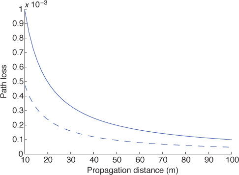
Figure 2.4 Path loss as a function of distance, measured as the ratio of receive power to transmit power, assuming a free-space path-loss model with isotropic antennas. More details about this channel model are found in Chapter 5.
There are a variety of models for path loss. In free space, path loss is proportional to the square of the frequency carrier, meaning that the higher-frequency carrier causes a higher path loss, assuming the receive antenna aperture decreases with antenna frequency. Path loss also depends on how well the transmitter can “see” the receiver. Specifically, the decay rate with distance is larger when the transmitter and receiver are obstructed in what is called non-line-of-sight (NLOS) propagation and is smaller when they experience line-of-sight (LOS) propagation. Several parameters like terrain, foliage, obstructions, and antenna heights are often taken into account in the computation of path loss. The path loss can even incorporate a random component, called shadowing, to account for variability of the received signal due to scattering objects in the environment.
A simple signal processing model for path loss is to scale the received signal by ![]() where the square root is to remind us that path loss is usually treated as a power. Modifying (2.1), the received signal with path loss and additive noise is
where the square root is to remind us that path loss is usually treated as a power. Modifying (2.1), the received signal with path loss and additive noise is
Path loss reduces the amplitude of the received signal, leading to a lower SNR.
2.3.4 Multipath Propagation
Radio waves traverse the propagation medium using mechanisms like diffraction, reflection, and scattering. In addition to the power loss described in the previous section, these phenomena cause the signal to propagate to the receiver via multiple paths. When there are multiple paths a signal can take between the transmitter and the receiver, the propagation channel is said to support multipath propagation, which results in multipath fading. These paths have different delays (due to different path lengths) and different attenuations, resulting in a smearing of the transmitted signal (similar to the effect of blurring an image).
There are different ways to model the effects of multipath propagation, depending on the bandwidth of the signal. In brief, if the bandwidth of the signal is small relative to a quantity called the coherence bandwidth, then multipath propagation creates an additional multiplicative impairment like the ![]() in (2.2), but it is modeled by a random process and varies over time. If the bandwidth of the signal is large, then multipath is often modeled as a convolution between the transmitted signal and the impulse response of the multipath channel. These models are described and the choice between models is explored further in Chapter 5.
in (2.2), but it is modeled by a random process and varies over time. If the bandwidth of the signal is large, then multipath is often modeled as a convolution between the transmitted signal and the impulse response of the multipath channel. These models are described and the choice between models is explored further in Chapter 5.
To illustrate the effects of multipath, consider a propagation channel with two paths. Each path introduces an attenuation α and a time delay τ. Modifying (2.2), the received signal with path loss, additive noise, and two multipaths is
The path loss ![]() is the same for both paths because it is considered to be a locally averaged quantity; additional differences in received power are captured in differences in α1 and α2. The smearing caused by multipath creates intersymbol interference, which must be mitigated at the receiver.
is the same for both paths because it is considered to be a locally averaged quantity; additional differences in received power are captured in differences in α1 and α2. The smearing caused by multipath creates intersymbol interference, which must be mitigated at the receiver.
Intersymbol interference (ISI) is a form of signal distortion resulting from multipath propagation as well as the distortion introduced by the analog filters. The name intersymbol interference means that the channel distortion is high enough that successively transmitted symbols interfere at the receiver; that is, a transmitted symbol arrives at the receiver during the next symbol period. Coping with this impairment is challenging when data is sent at high rates, since in these cases the symbol time is short and even a small delay can cause intersymbol interference. The effects of intersymbol interference are illustrated in Figure 2.5. The presence of ISI is usually analyzed using eye diagrams, as shown in this figure. The eye pattern overlaps many samples of the received signal. The effects of receiving several delayed and attenuated versions of the transmitted signal can be seen in the eye diagram as a reduction in the eye opening and loss of definition. Intersymbol interference can be mitigated by using equalization, as discussed in Chapter 5, or by using joint detection.

Figure 2.5 (a) Multipath propagation; (b) eye diagram corresponding to single-path propagation; (c) eye diagram corresponding to multipath propagation, showing ISI effects
2.4 Source Coding and Decoding
The main objective of a digital communication system is to transfer information. The source, categorized as either continuous or discrete, is the origin of this information. A continuous source is a signal with values taken from a continuum. Examples of continuous-valued sources include music, speech, and vinyl records. A discrete source has a finite number of possible values, usually a power of 2 and represented using binary. Examples of discrete sources include the 7-bit ASCII characters generated by a computer keyboard, English letters, and computer files. Both continuous and discrete sources may act as the origin of information in a digital communication system.
All sources must be converted into digital form for transmission by a digital communication system. To save the resources required to store and transport the information, as few bits as possible should be generated per unit time, with some distortion possibly allowed in the reconstruction. The objective of source coding is to generate a compressed sequence with as little redundancy as possible. Source decoding, as a result, reconstructs the original source from the compressed sequence, either perfectly or in a reasonable approximation.
Source coding includes both lossy and lossless compression. In lossy compression, some degradation is allowed to reduce the amount of resulting bits that need to be transmitted [35]. In lossless compression, redundancy is removed, but upon inverting the encoding algorithm, the signal is exactly the same [34, 345]. For discrete-time sources—for example, if f and g are the source encoding and decoding processes—then ![]() . For lossy compression,
. For lossy compression, ![]() , while for lossless compression,
, while for lossless compression, ![]() . Both lossy encoding and lossless encoding are used in conjunction with digital communication systems.
. Both lossy encoding and lossless encoding are used in conjunction with digital communication systems.
While source coding and decoding are important topics in signal processing and information theory, they are not a core part of the physical-layer signal processing in a wireless digital communication system. The main reason is that source coding and decoding often happen at the application layer, for example, the compression of video in a Skype call, which is far removed from the physical-layer tasks like error control coding and modulation. Consequently, we provide a review of the principles of source coding only in this section. Specialized topics like joint source-channel coding [78] are beyond the scope of this exposition. In the remainder of this book, we assume that source coding has already been performed. Specifically, we assume that ideal source coding has been accomplished such that the output of the source encoder is an independent identically distributed sequence of binary data.
2.4.1 Lossless Source Coding
Lossless source coding, also known as zero-error source coding, is a means of encoding a source such that it can be perfectly recovered without any errors. Many lossless source codes have been developed. Each source code is composed of a number of codewords. The codewords may have the same number of bits—for example, the ASCII code for computer characters, where each character is encoded by 7 bits. The codewords may also have different numbers of bits in what is called a variable-length code. Morse code is a classic variable-length code in which letters are represented by sequences of dots and dashes of different lengths. Lossless coding is ideal when working with data files where even a 1-bit error can corrupt the file.
The efficiency of a source-coding algorithm is related to a quantity called entropy, which is a function of the source’s alphabet and probabilistic description. Shannon showed that this source entropy is exactly the minimum number of bits per source symbol required for source encoding such that the corresponding source decoding can retrieve uniquely the original source information from the encoded string of bits. For a discrete source, the entropy corresponds to the average length of the codewords in the best possible lossless data compression algorithm. Consider a source that can take values from an alphabet with m distinct elements, each with probability p1, p2, · · · , pm. Then the entropy is defined as

where in the special case of a binary source
The entropy of a discrete source is maximized when all the symbols are equally likely, that is, pi = 1/m for i = 1, 2, . . . , m. A more complicated entropy calculation is provided in Example 2.1.
A discrete source generates an information sequence using the quaternary alphabet {a, b, c, d} with probabilities ![]() ,
, ![]() ,
, ![]() , and
, and ![]() . The entropy of the source is
. The entropy of the source is
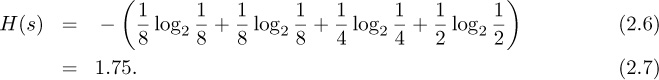
This means that lossless compression algorithms for encoding the source need at least 1.75 bits per alphabet letter.
There are several types of lossless source-coding algorithms. Two widely known in practice are Huffman codes and Lempel-Ziv (ZIP) codes. Huffman coding takes as its input typically a block of bits (often a byte). It then assigns a prefix-free variable-length codeword in such a way that the more likely blocks have smaller lengths. Huffman coding is used in fax transmissions. Lempel-Ziv coding is a type of arithmetic coding where the data is not segmented a priori into blocks but is encoded to create one codeword. Lempel-Ziv encoding is widely used in compression software like LZ77, Gzip, LZW, and UNIX compress. An illustration of a simple Huffman code is provided in Example 2.2.
Consider the discrete source given in Example 2.1. The Huffman coding procedure requires the forming of a tree where the branch ends correspond to the letters in the alphabet. Each branch is assigned a weight equal to the probability of the letter at the branch. Two branches with the lowest weights form a new branch whose weight is equal to the sum of the weights of the two branches. The procedure repeats with the new set of branches until forming the root with the weight of one. Each branch node is now labeled with a binary 1 or 0 decision to distinguish the two branches forming the node. The codeword for each letter is found by tracing the tree path from the root to the branching end where the letter is located. The procedure is illustrated in Figure 2.6.
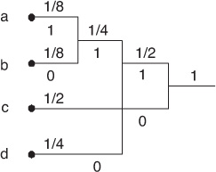
Figure 2.6 Huffman coding tree for the discrete source in Example 2.1
The codewords for the letters in the alphabet are as follows: 111 for a, 110 for b, 0 for c, and 10 for d. Notice that the letters with a higher probability correspond to the shorter codewords. Moreover, the average length of the codewords is 1.75 bits, exactly equal to the source entropy H(s).
2.4.2 Lossy Source Coding
Lossy source coding is a type of source coding where some information is lost during the encoding process, rendering perfect reconstruction of the source impossible. The purpose of lossy source coding is to reduce the average number of bits per unit time required to represent the source, at the expense of some distortion in the reconstruction. Lossy source coding is useful in cases where the end receiver of the information is human, as humans have some tolerance for distortion.
One of the most common forms of lossy source coding found in digital communication systems is quantization. Since continuous-time signals cannot be transmitted directly in a digital communication system, it is common for the source coding to involve sampling and quantization to generate a discrete-time signal from a continuous-time source. Essentially, the additional steps transform the continuous-time source into a close-to-equivalent digital source, which is then possibly further encoded. Note that these steps are the sources of errors in lossy source coding. In general, it is impossible to reconstruct uniquely and exactly the original analog sources from the resulting discrete source.
The sampling operation is based on the Nyquist sampling theorem, which is discussed in detail in Chapter 3. It says that no information is lost if a bandlimited continuous-time signal is periodically sampled with a small-enough period. The resulting discrete-time signal (with continuous-valued samples) can be used to perfectly reconstruct the bandlimited signal. Sampling, though, only converts the continuous-time signal to a discrete-time signal.
Quantization of the amplitudes of the sampled signals limits the number of possible amplitude levels, thus leading to data compression. For example, a B bit quantizer would represent a continuous-valued sample with one of 2B possible levels. The levels are chosen to minimize some distortion function, for example, the mean squared error. An illustration of a 3-bit quantizer is provided in Example 2.3.
Consider a 3-bit uniform quantizer. The dynamic range of the source, where most of the energy is contained, is assumed to be from −1 to 1. The interval [−1, 1] is then divided into 23 = 8 segments of the same length. Assuming the sampled signal is rounded to the closest end of the segment containing it, each sample is represented by the 3-bit codeword corresponding to the upper end of the segment containing the sample as illustrated in Figure 2.7. For example, a signal with a sample value of 0.44 is quantized to 0.375, which is in turn encoded by the codeword 101. The difference between 0.44 and 0.375 is the quantization error. Signals with values greater than 1 are mapped to the maximum value, in this case 0.875. This results in a distortion known as clipping. A similar phenomenon happens for signals with values less than −1.

There are several types of lossy coding beyond quantization. In other applications of lossy coding, the encoder is applied in a binary sequence. For example, the Moving Picture Experts Group (MPEG) defines various compressed audio and video coding standards used for digital video recording, and the Joint Photographic Experts Group (JPEG and JPEG2000) describes lossy still image compression algorithms, widely used in digital cameras [190].
2.5 Encryption and Decryption
Keeping the information transmitted by the source understandable by only the intended receivers is a typical requirement for a communication system. The openness of the wireless propagation medium, however, provides no physical boundaries to prevent unauthorized users from getting access to the transmitted messages. If the transmitted messages are not protected, unauthorized users are able not only to extract information from the messages (eavesdropping) but also to inject false information (spoofing). Eavesdropping and spoofing are just some implications of an insecure communication link.
In this section, we focus on encryption, which is one means to provide security against eavesdropping. Using encryption, the bit stream after source encoding is further encoded (encrypted) such that it can be decoded (decrypted) only by an intended receiver. This approach allows sensitive information to travel over a public network without compromising confidentiality.
There are several algorithms for encryption, and correspondingly for decryption. In this section, we focus on ciphers, which are widely used in communication. Ciphers work by transforming data using a known algorithm and a key or pair of keys. In secret-key encryption, an example of a symmetric cipher, a single secret key is used by both the encryption and the decryption. In public-key encryption, an example of an asymmetric cipher, a pair of keys is used: a public one for encryption and a private one for decryption. In a good encryption algorithm, it is difficult or ideally impossible to determine the secret or private key, even if the eavesdropper has access to the complete encryption algorithm and the public key. Informing the receiver about the secret or private key is a challenge in itself; it may be sent to the receiver by a separate and more secure means. Figure 2.8 illustrates a typical secret-key communication system [303].
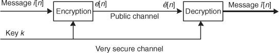
Now we describe a typical system. Let k1 denote the key used for encryption at the transmitter and k2 the key for decryption at the receiver. The mathematical model described in Section 2.2 for encryption should be revised as e[n] = p(i[n], k1), where p(·) denotes the cipher. At the receiver, the decrypted data can be written as ![]() , where q(·) is the corresponding decipher (i.e., the decrypting algorithm). In the case of public-key encryption, k1 and k2 are different from each other; k1 may be known to everyone, but k2 must be known by only the intended receiver. With secret-key encryption, k1 = k2 and the key remains unknown to the public. Most wireless communication systems use secret-key encryption because it is less computationally intensive; therefore we focus on secret-key encryption for the remainder of this section.
, where q(·) is the corresponding decipher (i.e., the decrypting algorithm). In the case of public-key encryption, k1 and k2 are different from each other; k1 may be known to everyone, but k2 must be known by only the intended receiver. With secret-key encryption, k1 = k2 and the key remains unknown to the public. Most wireless communication systems use secret-key encryption because it is less computationally intensive; therefore we focus on secret-key encryption for the remainder of this section.
Secret-key ciphers can be divided into two groups: block ciphers and stream ciphers [297]. Block ciphers divide the input data into nonoverlapping blocks and use the key to encrypt the data block by block to produce blocks of encrypted data of the same length. Stream ciphers generate a stream of pseudo-random key bits, which are then bitwise XORed (i.e., the eXclusive OR [XOR] operation) with the input data. Since stream ciphers can process the data byte after byte, and even bit after bit, in general they are much faster than block ciphers and more suitable to transmission of continuous and time-sensitive data like voice in wireless communication systems [297]. Moreover, a single bit error at the input of the block decrypter can lead to an error in the decryption of other bits in the same block, which is called error propagation. Stream ciphers are widely used in wireless, including GSM, IEEE 802.11, and Bluetooth, though the usage of block ciphers is also increasing with their incorporation into the 3GPP third- and fourth-generation cellular standards.
The major challenge in the design of stream ciphers is in the generation of the pseudo-random key bit sequences, or keystreams. An ideal keystream would be long, to foil brute-force attacks, but would still appear as random as possible. Many stream ciphers rely on linear feedback shift registers (LFSRs) to generate a fixed-length pseudo-random bit sequence as a keystream [297]. In principle, to create an LFSR, a feedback loop is added to a shift register of length n to compute a new term based on the previous n terms, as shown in Figure 2.9. The feedback loop is often represented as a polynomial of degree n. This ensures that the numerical operation in the feedback path is linear. Whenever a bit is needed, all the bits in the shift register are shifted right 1 bit and the LFSR outputs the least significant bit. In theory, an n-bit LFSR can generate a pseudo-random bit sequence of length up to (2n − 1) bits before repeating. LFSR-based keystreams are widely used in wireless communication, including the A5/1 algorithm in GSM [54], E0 in Bluetooth [44], the RC4 and AES algorithms [297] used in Wi-Fi, and even in the block cipher KASUMI used in 3GPP third- and fourth-generation cellular standards [101].

2.6 Channel Coding and Decoding
Both source decoding and decryption require error-free input data. Unfortunately, noise and other channel impairments introduce errors into the demodulation process. One way of dealing with errors is through channel coding, also called forward error correction or error control coding. Channel coding refers to a class of techniques that aim to improve communication performance by adding redundancy in the transmitted signal to provide resilience to the effects of channel impairments. The basic idea of channel coding is to add some redundancy in a controlled manner to the information bit sequence. This redundancy can be used at the receiver for error detection or error correction.
Detecting the presence of an error gives the receiver an opportunity to request a retransmission, typically performed as part of the higher-layer radio link protocol. It can also be used to inform higher layers that the inputs to the decryption or source decoding blocks had errors, and thus the outputs are also likely to be distorted. Error detection codes are widely used in conjunction with error correction codes, to indicate whether the decoded sequence is highly likely to be free of errors. The cyclic redundancy check (CRC) reviewed in Example 2.4 is the most widely used code for error detection.
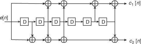
CRC codes operate on blocks of input data. Suppose that the input block length is k and that the output length is n. The length of the CRC, the number of parity bits, is n − k and the rate of the code is k/n. CRC operates by feeding the length k binary sequence into an LFSR that has been initialized to the zero state. The LFSR is parameterized by n − k weights w1, w2, . . . , wn−k. The operation of the LFSR is shown in Figure 2.10. The multiplies and adds are performed in binary. The D notation refers to a memory cell. As the binary data is clocked into the LFSR, the data in the memory cells is clocked out. Once the entire block has been input into the LFSR, the bits remaining in the memory cells form the length n − k parity. At the receiver, the block of bits can be fed into a similar LFSR and the resulting parity can be compared with the received parity to see if an error was made. CRC codes are able to detect about 1−2−(n−k) errors.

Error control codes allow the receiver to reconstruct an error-free bit sequence, if there are not too many errors. In general, a larger number of redundant bits allows the receiver to correct for more errors. Given a fixed amount of communication resources, though, more redundant bits means fewer resources are available for transmission of the desired information bits, which means a lower transmission rate. Therefore, there exists a trade-off between the reliability and the rate of data transmission, which depends on the available resources and the channel characteristics. This trade-off is illustrated through the simplest error control code, known as repetition coding, in Example 2.5. The example shows how a repetition code, which takes 1 bit and produces 3 output bits (a rate 1/3 code), is capable of correcting one error with a simple majority vote decoder. The repetition code is just one illustration of an error control code. This section reviews other types of codes, with a more sophisticated mathematical structure, that are more efficient than the repetition code.
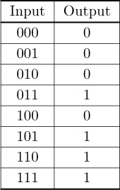
Consider a rate 1/3 repetition code. The code operates according to the mapping in Table 2.1. For example, if the bit sequence to be sent is 010, then the encoded sequence is 000111000.

Suppose that the decoder uses the majority decoding rule for decoding. This leads to the decoder mapping in Table 2.2. Based on the decoding table, if there is only one bit error, then the decoder outputs the correctly sent bit. If there are two or three bit errors, then the decoder decides in favor of the incorrectly sent bit and an error is made.
The performance of the code is often measured in terms of the probability of bit error. Suppose that a bit error occurs with probability p and is memoryless. The probability that 2 or 3 bits are in error out of a group of 3 bits is 1−(1−p)3 + 3p(1−p)2. For p = 0.01, the uncoded system sees an error probability of 0.01, which means on average one in 100 bits is in error. The coded system, though, sees an error probability of 0.000298, which means that on average about 3 bits in 10,000 are in error.
While repetition coding provides error protection, it is not necessarily the most efficient code. This raises an important issue, that is, how to quantify the efficiency of a channel code and how to design codes to achieve good performance. The efficiency of a channel code is usually characterized by its code rate k/n, where k is the number of information bits and n is the sum of the information and redundant bits. A large code rate means there are fewer redundant bits but generally leads to worse error performance. A code is not uniquely specified by its rate as there are many possible codes with the same rate that may possess different mathematical structures. Coding theory is broadly concerned with the design and analysis of error control codes.
Coding is fundamentally related to information theory. In 1948, Shannon proposed the concept of channel capacity as the highest information rate that can be transmitted through a channel with an arbitrarily small probability of error, given that power and bandwidth are fixed [302]. The channel capacity can be expressed as a function of a channel’s characteristics and the available resources. Let C be the capacity of a channel and R the information rate. The beauty of the channel capacity result is that for any noisy channel there exist channel codes (and decoders) that make it possible to transmit data reliably with the rate R < C. In other words, the probability of error can be as small as desired as long as the rate of the code (captured by R) is smaller than the capacity of the channel (measured by C). Furthermore, if R > C, there is no channel code that can achieve an arbitrarily small probability of error. The main message is that there is a bound on how large R can be (remember that since R = k/n, larger R means smaller n − k), which is determined by a property of the channel given by C. Since Shannon’s paper, much effort has been spent on designing channel codes that can achieve the limits he set out. We review a few strategies for error control coding here.
Linear block codes are perhaps the oldest form of error control coding, beyond simply repetition coding. They take a block of data and add redundancy to create a longer block. Block codes generally operate on binary data, performing the encoding either in the binary field or in a higher-order finite field. Codes that operate using a higher-order finite field have burst error correction capability since they treat groups of bits as an element of the field. Systematic block codes produce a codeword that contains the original input data plus extra parity information. Nonsystematic codes transform the input data into a new block. The well-known Hamming block code is illustrated in Example 2.6.
Various block codes are used in wireless communication. Fire codes [108], cyclic binary codes capable of burst error correction, are used for signaling and control in GSM [91]. Reed-Solomon codes [272] operate in a higher-order finite field and are typically used for correcting multiple burst errors. They have been widely used in deep-space communication [114] and more recently in WiMAX [244] and IEEE 802.11ad [162].
In this example we introduce the Hamming (7,4) code and explain its operation. The Hamming (7,4) code encodes blocks of 4 information bits into blocks of 7 bits by adding 3 parity/redundant bits into each block [136]. The code is characterized by the code generator matrix
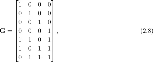
which takes an input vector of 4 bits e to produce an output vector of 7 bits c = Ge, where the multiplication and addition happen in the binary field. Note that it is conventional in coding to describe this operation using row vectors, but to be consistent within this book we explain it using column vectors. The code generator contains the 4 × 4 identity matrix, meaning that this is a systematic code.
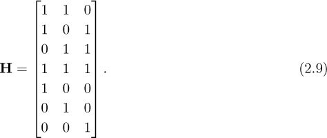
The parity check matrix for a linear block code is a matrix H such that HTG = 0. For the Hamming code
Now suppose that the observed data is ![]() where v is a binary error sequence (being all zero means there is no error). Then
where v is a binary error sequence (being all zero means there is no error). Then
If ![]() is not zero, then the received signal does not pass the parity check. The remaining component is called the syndrome, based on which the channel decoder can look for the correctable error patterns. The Hamming code is able to correct 1-bit errors, and its rate of 4/7 is much more efficient than the rate 1/3 repetition code that performs the same task.
is not zero, then the received signal does not pass the parity check. The remaining component is called the syndrome, based on which the channel decoder can look for the correctable error patterns. The Hamming code is able to correct 1-bit errors, and its rate of 4/7 is much more efficient than the rate 1/3 repetition code that performs the same task.
Another major category of channel coding found in wireless communications is convolutional coding. A convolutional code is in general described by a triple (k, n, K), where k and n have the same meaning as in block codes and K is the constraint length defining the number of k-tuple stages stored in the encoding shift register, which is used to perform the convolution. In particular, the n-tuples generated by a (k, n, K) convolutional code are a function not only of the current input k-tuple but also of the previous (K − 1) input k-tuples. K is also the number of memory elements needed in the convolutional encoder and plays a significant role in the performance of the code and the resulting decoding complexity. An example of a convolutional encode is shown in Example 2.7.
Convolutional codes can be applied to encode blocks of data. To accomplish this, the memory of the encoder is initialized to a known state. Often it is initialized to zero and the sequence is then zero padded (an extra K zeros are added to the block) so that it ends in the zero state. Alternatively, tail biting can be used where the code is initialized using the end of the block. The choice of initialization is explained in the decoding algorithm.
In this example we illustrate the encoding operation for a 64-state rate 1/2 convolutional code used in IEEE 802.11a as shown in Figure 2.11. This encoder has a single input bit stream (k = 1) and two output bit streams (n = 2). The shift register has six memory elements corresponding to 26 = 64 states. The connections of the feedback loops are defined by octal numbers as 1338 and 1718, corresponding to the binary representations 001011011 and 001111001. Two sets of output bits are created,
where ⊕ is the XOR operation. The encoded bit sequence is generated by interleaving the outputs, that is, c[2n] = c1[n] and c[2n + 1] = c2[n].
Decoding a convolutional code is challenging. The optimum approach is to search for the sequence that is closest (in some sense) to the observed error sequence based on some metric, such as maximizing the likelihood. Exploiting the memory of convolutional codes, the decoding can be performed using a forward-backward recursion known as the Viterbi algorithm [348]. The complexity of the algorithm is a function of the number of states, meaning that the error correction capability that results from longer constraint lengths comes at a price of more complexity.
Convolutional coding is performed typically in conjunction with bit interleaving. The reason is that convolutional codes generally have good random error correction capability but are not good with burst errors. They may also be combined with block codes that have good burst error correction capability, like the Reed-Solomon code, in what is known as concatenated coding. Decoding performance can be further improved by using soft information, derived from the demodulation block. When soft information is used, the output of the demodulator ![]() is a number that represents the likelihood that
is a number that represents the likelihood that ![]() is a zero or a one, as opposed to a hard decision that is just a binary digit. Most modern wireless systems use bit interleaving and soft decoding.
is a zero or a one, as opposed to a hard decision that is just a binary digit. Most modern wireless systems use bit interleaving and soft decoding.
Convolutional codes with interleaving have been widely used in wireless systems. GSM uses a constraint length K = 5 code for encoding data packets. IS-95 uses a constraint length K = 9 code for data. IEEE 802.11a/g/n use a constraint length K = 7 code as the fundamental channel coding, along with puncturing to achieve different rates. 3GPP uses convolutional codes with a constraint length K = 9 code.
Other types of codes are becoming popular for wireless communication, built on the foundations of iterative soft decoding. Turbo codes [36] use a modified recursive convolutional coding structure with interleaving to achieve near-optimal Shannon performance in Gaussian channels, at the expense of long block lengths. They are used in the 3GPP cellular standards. Low-density parity check (LDPC) codes [217, 314] are linear block codes with a special structure that, when coupled with efficient iterative decoders, also achieve near-optimal Shannon performance. They are used in IEEE 802.11ac and IEEE 802.11ad [259]. Finally, there has been interest in the recently developed polar codes [15], which offer options for lower-complexity decoding with good performance, and will be used for control channels in 5G cellular systems.
While channel coding is an important part of any communication system, in this book we focus on the signal processing aspects that pertain to modulation and demodulation. Channel coding is an interesting topic in its own right, already the subject of many textbooks [200, 43, 352]. Fortunately, it is not necessary to become a coding expert to build a wireless radio. Channel encoders and decoders are available in simulation software like MATLAB and LabVIEW and can also be acquired as intellectual property cores when implementing algorithms on an FPGA or ASIC [362, 331].
2.7 Modulation and Demodulation
Binary digits, or bits, are just an abstract concept to describe information. In any communication system, the physically transmitted signals are necessarily analog and continuous time. Digital modulation is the process at the transmit side by which information bit sequences are transformed into signals that can be transmitted over wireless channels. Digital demodulation is then the process at the receive side to extract the information bits from the received signals. This section provides a brief introduction to digital modulation and demodulation. Chapter 4 explores the basis of modulation and demodulation in the presence of additive white Gaussian noise, and Chapter 5 develops extended receiver algorithms for working with impairments.
There are a variety of modulation strategies in digital communication systems. Depending on the type of signal, modulation methods can be classified into two groups: baseband modulation and passband modulation. For baseband modulation, the signals are electrical pulses, but for passband modulation they are built on radio frequency carriers, which are sinusoids.
2.7.1 Baseband Modulation
In baseband modulation, the information bits are represented by electric pulses. We assume the information bits require the same duration of transmission, called a bit time slot. One simple method of baseband modulation is that 1 corresponds to bit time slots with the presence of a pulse and 0 corresponds to bit time slots without any pulse. At the receiver, the determination is made as to the presence or absence of a pulse in each bit time slot. In practice, there are many pulse patterns. In general, to increase the chance of detecting correctly the presence of a pulse, the pulse is made as wide as possible at the expense of a lower bit rate. Alternatively, signals can be described as a sequence of transitions between two voltage levels (bipolar). For example, a higher voltage level corresponds to 1 and a lower voltage level corresponds to 0. Alternate pulse patterns may have advantages including more robust detection or easier synchronization.
We consider two examples of baseband modulation: the non-return-to-zero (NRZ) code and the Manchester code. In NRZ codes, two nonzero different voltage levels H and L are used to represent the bits 0 and 1. Nevertheless, if the voltage is constant during a bit time slot, then a long sequence of all zeros or all ones can lead to loss of synchronization since there are no transitions in voltage to demarcate bit boundaries. To avoid this issue, the Manchester code uses the pulse with transitions that are twice as fast as the bit rate. Figure 2.12 illustrates the modulated signals for a bit sequence using the NRZ code and the Manchester code.

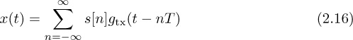
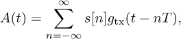
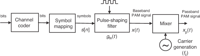
In principle, a pulse is characterized by its amplitude, position, and duration. These features of a pulse can be modulated by the information bits, leading to the corresponding modulation methods, namely, pulse-amplitude modulation (PAM), pulse-position modulation (PPM), and pulse-duration modulation (PDM). In this book we focus on complex pulse-amplitude modulations, which consist of two steps. In the first step, the bit sequence is converted into sequences of symbols. The set of all possible symbols is called the signal constellation. In the second step, the modulated signals are synthesized based on the sequence of symbols and a given pulse-shaping function. The entire process is illustrated in Figure 2.13 for the simplest case of real symbols. This is the well-known baseband modulation method called M-ary PAM.
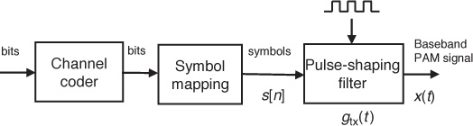
A pulse-amplitude modulated received signal at baseband may be written in the binary case as
where i[n] is the binary information sequence, gtx(t) is the transmit pulse shape, T is the symbol duration, and υ(t) is additive noise (typically modeled as random). In this example, i[n] = 0 becomes a “1” symbol, and i[n] = 1 becomes a “−1” symbol.
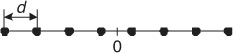
In M-ary PAM one of M allowable amplitude levels is assigned to each of the M symbols of the signal constellation. A standard M-ary PAM signal constellation C consists of M d-spaced real numbers located symmetrically around the origin, that is,

where d is the normalization factor. Figure 2.14 illustrates the positions of the symbols for an 8-PAM signal constellation. The modulated signal corresponding to the transmission of a sequence of M real symbols using PAM modulation can be written as the summation of uniform time shifts of the pulse-shaping filter multiplied by the corresponding symbol
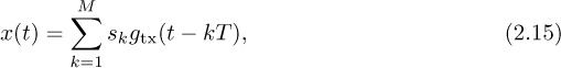
where T is the interval between the successive symbols and sk is the kth transmitted symbol, which is selected from CPAM based on the information sequence i[n].
The transmitter outputs the modulated signals to the wireless channel. Baseband signals, which are produced by baseband modulation methods, are not efficient because the transmission through the space of the electromagnetic fields corresponding to low baseband frequencies requires very large antennas. Therefore, all practical wireless systems use passband modulation methods.
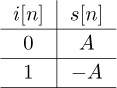
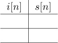
Binary phase-shift keying (BPSK) is one of the simplest forms of digital modulation. Let i[n] denote the sequence of input bits, s[n] a sequence of symbols, and x(t) the continuous-time modulated signal. Suppose that bit 0 produces A and bit 1 produces −A.
• Create a bit-to-symbol mapping table.
Answer:
• BPSK is a type of pulse-amplitude modulation. Let gtx(t) denote the pulse shape and let
denote the modulated baseband signal. Let the pulse ![]() for t ∈ [0, T] and gtx(t) = 0 otherwise. Draw a graph of x(t) for the input i[0] = 1, i[1] = 1, i[2] = 0, i[3] = 1, with A = 3 and T = 2. Illustrate for t ∈ [0, 8].
for t ∈ [0, T] and gtx(t) = 0 otherwise. Draw a graph of x(t) for the input i[0] = 1, i[1] = 1, i[2] = 0, i[3] = 1, with A = 3 and T = 2. Illustrate for t ∈ [0, 8].
Answer: The illustration is found in Figure 2.15.
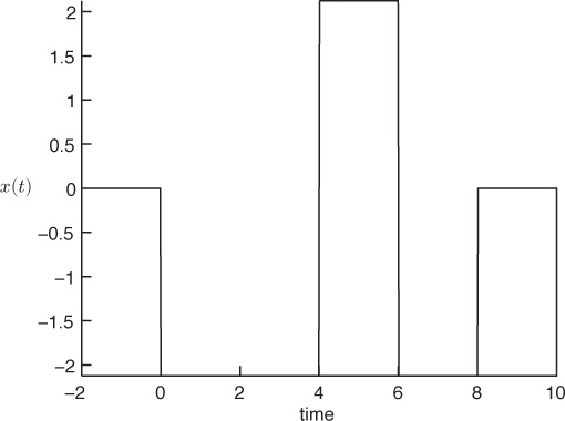
Figure 2.15 Output of a BPSK modulator when the transmit pulse-shaping filter is a rectangular function
2.7.2 Passband Modulation
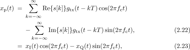
The signals used in passband modulation are RF carriers, which are sinusoids. Sinusoids are characterized by their amplitude, phase, and frequency. Digital passband modulation can be defined by the process whereby any features, or any combination of features, of an RF carrier are varied in accordance with the information bits to be transmitted. In general, a passband modulated signal xp(t) can be expressed as follows:
where A(t) is the time-varying amplitude, fc is the frequency carrier in hertz, and ϕ(t) is the time-varying phase. Several of the most common digital passband modulation types are amplitude-shift keying (ASK), phase-shift keying (PSK), frequency-shift keying (FSK), and quadrature-amplitude modulation (QAM).
In ASK modulation methods, only the amplitude of the carrier is changed according to the transmission bits. The ASK signal constellation is defined by different amplitude levels:
Therefore, the resulting modulated signal is given by
where fc and ϕ0 are constant; T is the symbol duration time, and
where s(n) is drawn from CASK. Figure 2.16 shows the block diagram of a simple ASK modulator.
The PSK modulation methods transmit information by changing only the phase of the carrier while the amplitude is kept constant (we can assume the amplitude is 1). The modulation is done by the phase term as follows:
where ϕ(t) is a signal that depends on the sequence of bits. Quadrature PSK (QPSK) and 8-PSK are the best-known PSK modulations. 8-PSK modulation is often used when there is a need for a 3-bit constellation, for example, in the GSM and EDGE (Enhanced Data rates for GSM Evolution) standards.
In FSK modulation, each vector symbol is represented by a distinct frequency carrier fk for k = 1, 2, · · · , M. For example, it may look like
This modulation method thus requires the availability of a number of frequency carriers that can be distinguished from each other.
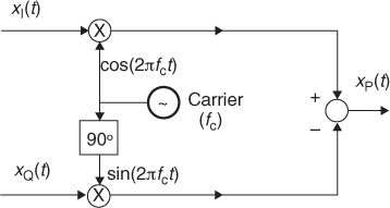
The most commonly used passband modulation is M-QAM modulation. QAM modulation changes both the amplitude and the phase of the carrier; thus it is a combination of ASK and PSK. We can also think of an M-QAM constellation as a two-dimensional constellation with complex symbols or a Cartesian product of two M/2-PAM constellations. QAM modulated signals are often represented in the so-called IQ form as follows:
where xI(t) and xQ(t) are the M/2-PAM modulated signals for the inphase and quadrature components. M-QAM is described more extensively in Chapter 4.
Figure 2.17 shows the block diagram of a QAM modulator. M-QAM modulation is used widely in practical wireless systems such as IEEE 802.11 and IEEE 802.16.
This example considers BPSK with passband modulation, continuing Example 2.10. For BPSK, the passband signal is denoted as
where x(t) is defined in (2.16). BPSK is a simplification of M-QAM with only an inphase component. The process of creating xp(t) from x(t) is known as upconversion.
• Plot xp(t) for t ∈ [0, 8] and interpret the results. Choose a reasonable value of fc so that it is possible to interpret your plot.
Answer: Using a small value of fc shows the qualitative behavior of abrupt changes in Figure 2.18. The signal changes phase at the points in time when the bits change. Essentially, information is encoded in the phase of the cosine, rather than in its amplitude. Note that with more complicated pulse-shaping functions, there would be more amplitude variation.

Figure 2.18 Output of a BPSK modulator with a square pulse shape from Example 2.11 when the carrier frequency is very small (just for illustration purposes)
• The receiver in a wireless system usually operates on the baseband signal. Neglecting noise, suppose that the received signal is the same as the transmit signal. Show how to recover x(t) from xp(t) by multiplying by cos(2πfct) and filtering.
Answer: After multiplying xp(t) by cos(2πfct),
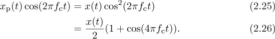
The carrier at 2fc can be removed by a lowpass-filtering (LPF) operation, so that the output of the filter is a scaled version of x(t).
2.7.3 Demodulation with Noise
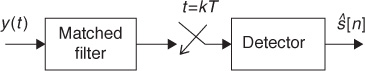
When the channel adds noise to the passband modulated signal that passes through it, the symbol sequence can be recovered by using a technique known as matched filtering, as shown in Figure 2.19. The receiver filters the received signal y(t) with a filter whose shape is “matched” to the transmitted signal’s pulse shape gtx(t). The matched filter limits the amount of noise at the output, but the frequencies containing the data signal are passed. The output of the matched filter is then sampled at multiples of the symbol period. Finally, a decision stage finds the symbol vector closest to the received sample. This demodulation procedure and the mathematical definition of the matched filter are covered in detail in Chapter 4. In practical receivers this is usually implemented in digital, using sampled versions of the received signal and the filter.
In this example we consider the baseband BPSK signal from Example 2.10. A simple detector is based on the matched filter, which in this example is the transmit rectangular pulse gtx(t) in Example 2.10.
• Show that ![]() where x(t) is given in (2.16).
where x(t) is given in (2.16).
Answer:
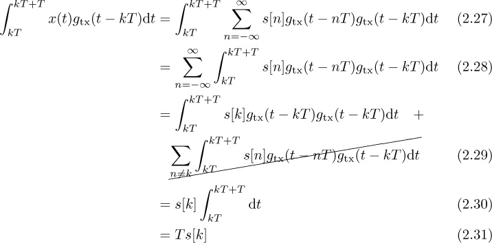
The original signal can be recovered by dividing by T.
• Plot the signal at the output of the matched filter, which is also a rectangular pulse, in t ∈ [−2, 10], when x(t) is the baseband BPSK signal from Example 2.10 corrupted by noise. Plot the sampled received signal at t = 1, 3, 5, 7. Interpret the results.
Answer: Figure 2.20(a) shows the output of the matched filter for the signal x(t) in Example 2.10 corrupted by additive noise. The samples of the received signal at multiples of the symbol period are represented in Figure 2.20(b) to show the output of the sampling stage. Then, the detector has to find the closest symbol to this received vector. Despite the noise, the detector provides the right symbol sequence [−1, −1, 1, −1].
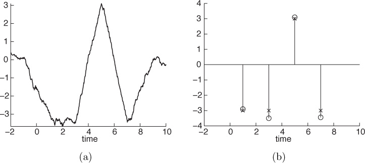
Figure 2.20 (a) Output of the matched filter for the signal in Example 2.10 corrupted by noise; (b) output samples of the sampling stage after the matched filter (circles) and transmitted symbols (x-marks)
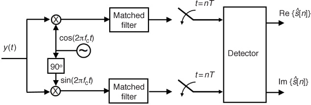
When demodulating a general passband signal, we need to extract the symbol information from the phase or the amplitude of an RF carrier. For M-QAM, the demodulator operates with two basic demodulators in parallel to extract the real and imaginary parts of the symbols. This demodulator can be implemented as shown in Figure 2.21. The passband received signal y(t) is corrupted by noise as in the baseband case, and the matched filters remove noise from both components.
In practice, however, the channel output signal is not equal to the modulated signal plus a noise term; signal distortion is also present, thus requiring more complicated demodulation methods, which are briefly described in Section 2.7.4 and discussed in detail in Chapter 5.
2.7.4 Demodulation with Channel Impairments
Real wireless channels introduce impairments besides noise in the received signal. Further, other functional blocks have to be added to the previous demodulation structures to recover the transmitted symbol. Moreover, practical realizations of the previous demodulators require the introduction of additional complexity in the receiver.
Consider, for example, the practical implementation of the demodulation scheme in Figure 2.19. It involves sampling at a time instant equal to multiples of the symbol duration, so it is necessary to find somehow the phase of the clock that controls this sampling. This is the so-called symbol timing recovery problem. Chapter 5 explains the main approaches for estimating the optimal sampling phase in systems employing complex PAM signals.
In a practical passband receiver some additional problems appear. The RF carriers used at the modulator are not exactly known at the receiver in Figure 2.21. For example, the frequency generated by the local oscillator at the receiver may be slightly different than the transmit frequency, and the phase of the carriers will also be different. Transmission through the wireless channel may also introduce a frequency offset in the carrier frequency due to the Doppler effect. Figure 2.22 shows the effect of a phase offset in a QPSK constellation. Because of these variations, a practical M-QAM receiver must include carrier phase and frequency estimation algorithms to perform the demodulation. Chapter 5 describes the main approaches for phase and frequency offset correction for single-carrier and OFDM systems.

Consider BPSK with passband modulation, continuing Example 2.11. Suppose that during the downconversion process, the receiver multiplies by cos(2π(fc + ![]() )t), where
)t), where ![]() ≠ 0 represents the frequency offset. Show how the received signal, in the absence of noise, is distorted.
≠ 0 represents the frequency offset. Show how the received signal, in the absence of noise, is distorted.
Answer:
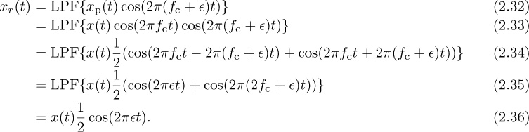
Because of the term cos(2π![]() t) in the demodulated signal, reconstruction by simple filtering no longer works, even for small values of
t) in the demodulated signal, reconstruction by simple filtering no longer works, even for small values of ![]() .
.
As described in Section 2.3, the wireless channel also introduces multipath propagation. The input of the demodulator is not the modulated signal x(t) plus a noise term, but it includes a distorted version of x(t) because of multipath. This filtering effect introduced by the channel has to be compensated at the receiver using an equalizer. Chapter 5 introduces the basis for the main channel equalization techniques used in current digital communication systems.
2.8 Summary
• Both analog and digital communication send information using continuous-time signals.
• Digital communication is well suited for digital signal processing.
• Source coding removes the redundancy in the information source, reducing the number of bits that need to be transmitted. Source decoding reconstructs the uncompressed sequence either perfectly or with some loss.
• Encryption scrambles data so that it can be decrypted by the intended receiver, but not by an eavesdropper.
• Channel coding introduces redundancy that the channel decoder can exploit to reduce the effects of errors introduced in the channel.
• Shannon’s capacity theorem gives an upper bound on the rate that can be supported by a channel with an arbitrarily low probability of error.
• Significant impairments in a wireless communication system include additive noise, path loss, interference, and multipath propagation.
• Physically transmitted signals are necessarily analog. Digital modulation is the process by which bit sequences containing the information are transformed into continuous signals that can be transmitted over the channel.
• Demodulating a signal consists of extracting the information bits from the received waveform.
• Sophisticated signal processing algorithms are used at the receiver side to compensate for the channel impairments in the received waveform.
Problems
1. Short Answer
(a) Why should encryption be performed after source coding?
(b) Why are digital communication systems implemented in digital instead of completely in analog?
2. Many wireless communication systems support adaptive modulation and coding, where the code rate and the modulation order (the number of bits per symbol) are adapted over time. Periodic puncturing of a convolutional code is one way to adapt the rate. Do some research and explain how puncturing works at the transmitter and how it changes the receiver processing.
3. A discrete source generates an information sequence using the ternary alphabet {a, b, c} with probabilities ![]() ,
, ![]() , and
, and ![]() . How many bits per alphabet letter are needed for source encoding?
. How many bits per alphabet letter are needed for source encoding?
4. Look up the stream ciphering used in the original GSM standard. Draw a block diagram that corresponds to the cipher operation and also give a linear feedback shift register implementation.
5. Determine the CRC code used in the WCDMA (Wideband Code Division Multiple Access) cellular system, the first release of the third-generation cellular standard.
(a) Find the length of the code.
(b) Give a representation of the coefficients of the CRC code.
(c) Determine the error detection capability of the code.
6. Linear Block Code Error control coding is used in all digital communication systems. Because of space constraints, we do not cover error control codes in detail in this book. Linear block codes refer to a class of parity-check codes that independently transform blocks of k information bits into longer blocks of m bits. This problem explores two simple examples of such codes.
Consider a Hamming (6,3) code (6 is the codeword length, and 3 is the message length in bits) with the following generator matrix:

(a) Is this a systematic code?
(b) List all the codewords for this (6,3) code. In other words, for every possible binary input of length 3, list the output. Represent your answer in table form.
(c) Determine the minimum Hamming distance between any two codewords in the code. The Hamming distance is the number of bit locations that differ between two locations. A code can correct c errors if the Hamming distance between any two codewords is at least 2c + 1.
(d) How many errors can this code correct?
(e) Without any other knowledge of probability or statistics, explain a reasonable way to correct errors. In other words, there is no need for any mathematical analysis here.
(f) Using the (6,3) code and your reasonable method, determine the number of bits you can correct.
(g) Compare your method and the rate 1/3 repetition code in terms of efficiency.
7. HDTV Do some research on the ATSC HDTV broadcast standard. Be sure to cite your sources in the answers. Note: You should find some trustworthy sources that you can reference (e.g., there may be mistakes in the Wikipedia article or it may be incomplete).
(a) Determine the types of source coding used for ATSC HDTV transmission. Create a list of different source coding algorithms, rates, and resolutions supported.
(b) Determine the types of channel coding (error control coding) used in the standard. Provide the names of the different codes and their parameters, and classify them as block code, convolution code, trellis code, turbo code, or LDPC code.
(c) List the types of modulation used for ATSC HDTV.
8. DVB-H Do some research on the DVB-H digital broadcast standard for handheld devices. Be sure to cite your sources in the answers. Note: You should find some trustworthy sources that you can reference (e.g., there may be mistakes in the Wikipedia article or it may be incomplete).
(a) Determine the types of source coding used for DVB-H transmission. Create a list of different source coding algorithms, rates, and resolutions supported.
(b) Determine the types of channel coding (error control coding) used in the standard. Provide the names of the different codes and their parameters, and classify them as block code, convolution code, trellis code, turbo code, or LDPC code.
(c) List the types of modulation used for DVB-H.
(d) Broadly speaking, what is the relationship between DVB and DVB-H?
9. On-off keying (OOK) is another form of digital modulation. In this problem, you will illustrate the operation of OOK. Let i[n] denote the sequence of input bits, s[n] a sequence of symbols, and x(t) the continuous-time modulated signal.
(a) Suppose that bit 0 produces 0 and bit 1 produces A. Fill in the bit mapping table.
(b) OOK is a type of amplitude modulation. Let g(t) denote the pulse shape and let
denote the modulated baseband signal. Let g(t) be a triangular pulse shape function defined as
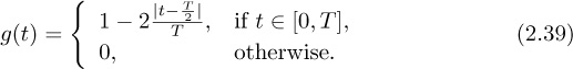
Draw a graph of x(t) for the input i[0] = 1, i[1] = 1, i[2] = 0, i[3] = 1, with A = 4 and T = 2. You can illustrate for t ∈ [0, 8]. Please draw this by hand.
(c) Wireless communication systems use passbands signals. Let the carrier frequency fc = 1GHz. For OOK, the passband signal is
Plot x(t) for the same range as the previous plot. Be careful! You might want to plot using a computer program, such as MATLAB or LabVIEW. Explain how the information is encoded in this case versus the previous case. The process of going from x(t) to xp(t) is known as upconversion. Illustrate the qualitative behavior with a smaller value of fc.
(d) The receiver in a wireless system usually operates on the baseband signal. Neglect to noise, suppose that the received signal is the same as the transmit signal. Show how to recover x(t) from xp(t) by multiplying xp(t) by cos(2πfct) and filtering.
(e) What happens if you multiply instead by cos(2π(fc + ![]() )t) where
)t) where ![]() ≠ 0? Can you still recover x(t)?
≠ 0? Can you still recover x(t)?
(f) A simple detector is the matched filter. Show that ![]() .
.
(g) What happens if you compute ![]() , where τ ∈ (0, T)?
, where τ ∈ (0, T)?
10. M-ary PAM is a well-known baseband modulation method in which one of M allowable amplitude levels is assigned to each of the M vector symbols of the signal constellation. A standard 4-PAM signal constellation consists of four real numbers located symmetrically around the origin, that is,

Since there are four possible levels, one symbol corresponds to 2 bits of information. Let i[n] denote the sequence of input bits, s[n] a sequence of symbols, and x(t) the continuous-time modulated signal.
(a) Suppose we want to map the information bits to constellation symbols by their corresponding numeric ordering. For example, among the four possible binary sequences of length 2, 00 is the smallest, and among the constellation symbols, ![]() is the smallest, so we map 00 to
is the smallest, so we map 00 to ![]() . Following this pattern, complete the mapping table below:
. Following this pattern, complete the mapping table below:

(b) Let g(t) denote the pulse shape and let
denote the modulated baseband signal. Let g(t) be a triangular pulse shape function defined as
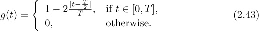
By hand, draw a graph of x(t) for the input bit sequence 11 10 00 01 11 01, with T = 2. You can illustrate for t ∈ [0, 12].
(c) In wireless communication systems, we send passband signals. The concept of passband signals is covered in Chapter 3. Let the carrier frequency be fc; then the passband signal is given by
For cellular systems, the range of fc is between 800MHz and around 2GHz. For illustration purposes here, use a very small value, fc = 2Hz. You might want to plot using a computer program such as MATLAB or LabVIEW. Explain how the information is encoded in this case versus the previous case.
(d) The receiver in a wireless system usually operates on the baseband signal. At this point we neglect noise and suppose that the received signal is the same as the transmit signal. Show how to recover x(t) from xp(t) by multiplying xp(t) by cos(2πfct) and filtering. The process of recovering a baseband signal from a passband signal is known as downconversion.
(e) What happens if you multiply instead by cos(2π(fc + ![]() )t), where
)t), where ![]() ≠ 0? Can you still recover x(t)? This is called carrier frequency offset and is covered in more detail in Chapter 5.
≠ 0? Can you still recover x(t)? This is called carrier frequency offset and is covered in more detail in Chapter 5.
(f) A simple detector is the matched filter. Show that ![]() .
.
(g) What happens if ![]() , where τ ∈ (0, T)? This is called symbol timing offset and is covered in more detail in Chapter 5.
, where τ ∈ (0, T)? This is called symbol timing offset and is covered in more detail in Chapter 5.