
Chapter 5. Dealing with Impairments
Communication in wireless channels is complicated, with additional impairments beyond AWGN and more elaborate signal processing to deal with those impairments. This chapter develops more complete models for wireless communication links, including symbol timing offset, frame timing offset, frequency offset, flat fading, and frequency-selective fading. It also reviews propagation channel modeling, including large-scale fading, small-scale fading, channel selectivity, and typical channel models.
We begin the chapter by examining the case of frequency-flat wireless channels, including topics such as the frequency-flat channel model, symbol synchronization, frame synchronization, channel estimation, equalization, and carrier frequency offset correction. Then we consider the ramifications of communication in considerably more challenging frequency-selective channels. We revisit each key impairment and present algorithms for estimating unknown parameters and removing their effects. To remove the effects of the channel, we consider several types of equalizers, including a least squares equalizer determined from a channel estimate, an equalizer directly determined from the unknown training, single-carrier frequency-domain equalization (SC-FDE), and orthogonal frequency-division multiplexing (OFDM). Since equalization requires an estimate of the channel, we also develop algorithms for channel estimation in both the time and frequency domains. Finally, we develop techniques for carrier frequency offset correction and frame synchronization. The key idea is to use a specially designed transmit signal to facilitate frequency offset estimation and frame synchronization prior to other functions like channel estimation and equalization. The approach of this chapter is to consider specific algorithmic solutions to these impairments rather than deriving optimal solutions.
We conclude the chapter with an introduction to propagation channel models. Such models are used in the design, analysis, and simulation of communication systems. We begin by describing how to decompose a wireless channel model into two submodels: one based on large-scale variations and one on small-scale variations. We then introduce large-scale models for path loss, including the log-distance and LOS/NLOS channel models. Next, we describe the selectivity of a small-scale fading channel, explaining how to determine if it is frequency selective and how quickly it varies over time. Finally, we present several small-scale fading models for both flat and frequency-selective channels, including some analysis of the effects of fading on the average probability of symbol error.
5.1 Frequency-Flat Wireless Channels
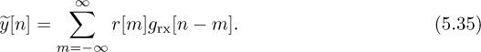
In this section, we develop the frequency-flat AWGN communication model, using a single-path channel and the notion of the complex baseband equivalent. Then we introduce several impairments and explain how to correct them. Symbol synchronization corrects for not sampling at the correct point, which is also known as symbol timing offset. Frame synchronization finds a known reference point in the data—for example, the location of a training sequence—to overcome the problem of frame timing offset. Channel estimation is used to estimate the unknown flat-fading complex channel coefficient. With this estimate, equalization is used to remove the effects of the channel. Carrier frequency offset synchronization corrects for differences in the carrier frequencies between the transmitter and the receiver. This chapter provides a foundation for dealing with impairments in the more complicated case of frequency-selective channels.
5.1.1 Discrete-Time Model for Frequency-Flat Fading
The wireless communication channel, including all impairments, is not well modeled simply by AWGN. A more complete model also includes the effects of the propagation channel and filtering in the analog front end. In this section, we consider a single-path channel with impulse response
Based on the derivations in Section 3.3.3 and Section 3.3.4, this channel has a complex baseband equivalent given by
and pseudo-baseband equivalent channel
See Example 3.37 and Example 3.39 to review this calculation. The Bsinc(t) term is present because the complex baseband equivalent is a baseband bandlimited signal. In the frequency domain
we observe that |H(f)| is a constant for f ∈ [−B/2, B/2]. This channel is said to be frequency flat because it is constant over the bandwidth of interest to the signal. Channels that consist of multipaths can be approximated as frequency flat if the signal bandwidth is much less than the coherence bandwidth, which is discussed further in Section 5.8.
Now we incorporate this channel into our received signal model. The channel in (5.2) convolves with the transmitted signal prior to the noise being added at the receiver. As a result, the complex baseband received signal prior to matched filtering and sampling is

To ensure that r(t) is bandlimited, henceforth we suppose that the noise has been lowpass filtered to have a bandwidth of B/2. For simplicity of notation, and to be consistent with the discrete-time representation, we let ![]() and write
and write

The factor of ![]() is included in h since only the combined scaling is important from the perspective of receiver design. Matched filtering and sampling at the symbol rate give the received signal
is included in h since only the combined scaling is important from the perspective of receiver design. Matched filtering and sampling at the symbol rate give the received signal

where g(t) is a Nyquist pulse shape. Compared with the AWGN received signal model y[n] = s[n] + υ[n], there are several sources of distortion, which must be recognized and corrected.
One impairment is caused by symbol timing error. Suppose that τd is a fraction of a symbol period, that is, τd ∈ [0, T). This models the effect of sample timing error, which happens when the receiver does not sample at precisely the right point in time. Under this assumption

Intersymbol interference is created when the Nyquist pulse shape is not sampled exactly at nT, since g(nT + τd) is not generally equal to δ[n]. Correcting for this fractional delay requires symbol synchronization, equalization, or a more complicated detector.
A second impairment occurs with larger delays. For illustration purposes, suppose that τd = dT for some integer d. This is the case where symbol timing has been corrected but an unknown propagation delay, which is a multiple of the symbol period, remains. Under this assumption
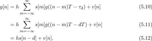
Essentially integer offsets create a mismatch between the indices of the transmitted and received symbols. Frame synchronization is required to correct this frame timing error impairment.
Finally, suppose that the unknown delay τd has been completely removed so that τd = 0. Then the received signal is
Sampling and removing delay leaves distortion due to the attenuation and phase shift in h. Dealing with h requires either a specially designed modulation scheme, like DQPSK (differential quadrature phase-shift keying), or channel estimation and equalization.
It is clear that amplitude, phase, and delay if not compensated can have a drastic impact on system performance. As a consequence, every wireless system is designed with special features to enable these impairments to be estimated or directly removed in the receiver processing. Most of this processing is performed on small segments of data called bursts, packets, or frames. We emphasize this kind of batch processing in this book. Many of the algorithms have adaptive extensions that can be applied to continually estimate impairments.
5.1.2 Symbol Synchronization
The purpose of symbol synchronization, or timing recovery, is to estimate and remove the fractional part of the unknown delay τd, which corresponds to the part of the error in [0, T). The theory behind these algorithms is extensive and their history is long [309, 226, 124]. The purpose of this section is to present one of the many algorithm approaches for symbol synchronization in complex pulse-amplitude modulated systems.
Philosophically, there are several approaches to synchronization as illustrated in Figure 5.1. There is a pure analog approach, a combined digital and analog approach where digital processing is used to correct the analog, and a pure digital approach. Following the DSP methodology, this book considers only the case of pure digital symbol synchronization.
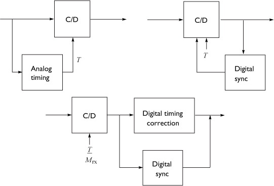
We consider two different strategies for digital symbol synchronization, depending on whether the continuous-to-discrete converter can be run at a low sampling rate or a high sampling rate:
• The oversampling method, illustrated in Figure 5.2, is suitable when the oversampling factor Mrx is large and therefore a high rate of oversampling is possible. In this case the synchronization algorithm essentially chooses the best multiple of T/Mrx and adds a suitable integer delay k* prior to downsampling.

• The resampling method is illustrated in Figure 5.3. In this case a resampler, or interpolator, is used to effectively create an oversampled signal with an effective sample period of T/Mrx even if the actual sampling is done with a period less than T/Mrx but still satisfying Nyquist. Then, as with the oversampling method, the multiple of T/Mrx is estimated and a suitable integer delay k* is added prior to the downsampling operation.

A proper theoretical approach for solving for the best of τd would be to use estimation theory. For example, it is possible to solve for the maximum likelihood estimator. For simplicity, this section considers an approach based on a cost function known as the maximum output energy (MOE) criterion, the same approach as in [169]. There are other approaches based on maximum likelihood estimation such as the early-late gate approach. Lower-complexity implementations of what is described are possible that exploit filter banks; see, for example, [138].
First we compute the energy output as a way to justify each approach for timing synchronization. Denote the continuous-time output of the matched filter as

The output energy after sampling by nT + τ is

Suppose that τd = dT + τfrac and ![]() ; then
; then
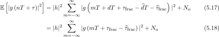
with a change of variables. Therefore, while the delay τ can take an arbitrary positive value, only the offset that corresponds to the fractional delay has an impact on the output energy.
The maximum output energy approach to symbol timing attempts to find the τ that maximizes JMOE(τ) where τ ∈ [0, T]. The maximum output energy solution is
The rationale behind this approach is that
where the inequality is true for most common pulse-shaping functions (but not for arbitrarily chosen pulse shapes). Thus the unique maximum of JMOE(τ) corresponds to τ = τd. The values of JMOE(τ) are plotted in Figure 5.4 for the raised cosine pulse shape. A proof of (5.20) for sinc and raised cosine pulse shapes is established in Example 5.1 and Example 5.2.
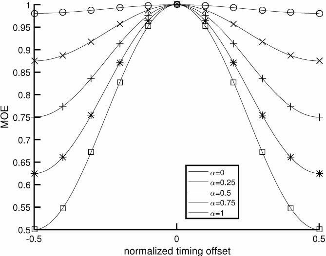
Figure 5.4 Plot of JMOE(τ) for τ ∈ [−T/2, T/2], in the absence of noise, assuming a raised cosine pulse shape (4.73). The x-axis is normalized to T. As the rolloff value of the raised cosine is increased, the output energy peaks more, indicating that the excess bandwidth provided by choosing larger values of rolloff α translates into better symbol timing using the maximum output energy cost function.
Show that the inequality in (5.20) is true for sinc pulse shapes.
Answer: For convenience denote

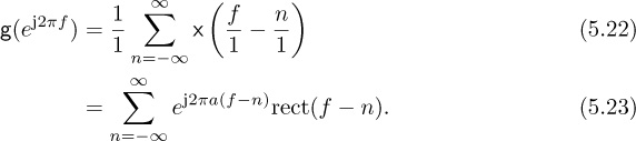
where ![]() . Let g(t) = sinc(t+a) and g[m] = g(mT) = sinc(m+a), and let
. Let g(t) = sinc(t+a) and g[m] = g(mT) = sinc(m+a), and let g(f) and g(ej2πf) be the CTFT of g(t) and DTFT of g[m] respectively. Then g(f) = ej2πaf rect(f) and
By Parseval’s theorem for the DTFT we have
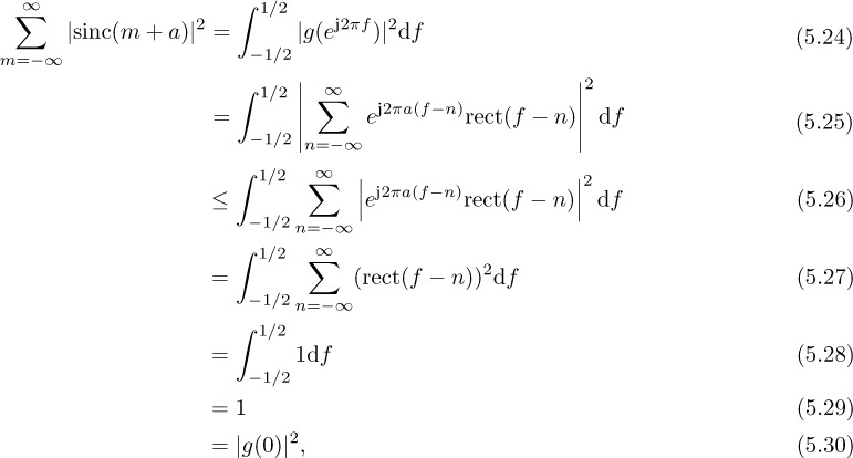
where the inequality follows because |∑ai| ≤ ∑ |ai|. Therefore,
Show that the MOE inequality in (5.20) holds for raised cosine pulse shapes.
Answer: The raised cosine pulse

is a modulated version of the sinc pulse shape. Since
it follows that
and the result from Example 5.1 can be used.
Now we develop the direct solution to maximizing the output energy, assuming the receiver architecture with oversampling as in Figure 4.10. Let r[n] denote the signal after oversampling or resampling, assuming there are Mrx samples per symbol period. Let the output of the matched receiver filter prior to downsampling at the symbol rate be
We use this sampled signal to compute a discrete-time version of JMOE(τ) given by
where k is the sample offset between 0, 1, . . . , Mrx − 1 corresponding to an estimate of the fractional part of the timing offset given by kT/Mrx. To develop a practical algorithm, we replace the expectation with a time average over P symbols, thanks to ergodicity, so that
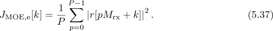
Looking for the maximizer of JMOE,e[k] over k = 0, 1, . . . , Mrx − 1 gives the optimum sample k* and an estimate of the symbol timing offset k*T/Mrx.
The optimum correction involves advancing the received signal by k* samples prior to downsampling. Essentially, the synchronized data is ![]() . Equivalently, the signal can be delayed by k* − Mrx samples, since subsequent signal processing steps will in any case correct for frame synchronization.
. Equivalently, the signal can be delayed by k* − Mrx samples, since subsequent signal processing steps will in any case correct for frame synchronization.
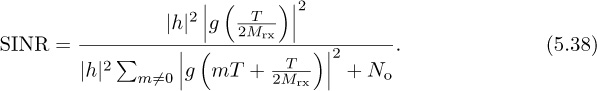
The main parameter to be selected in the symbol timing algorithms covered in this section is the oversampling factor Mrx. This decision can be based on the residual ISI created because the symbol timing is quantized. Using the SINR from (4.56), assuming h is known perfectly, matched filtering at the receiver, and a maximum symbol timing offset T/2Mrx, then
This value can be used, for example, with the probability of symbol error analysis in Section 4.4.5 to select a value of Mrx such that the impact of symbol timing error is acceptable, depending on the SNR and target probability of symbol error. An illustration is provided in Figure 5.5 for the case of 4-QAM. In this case, a value of Mrx = 8 leads to less than 1dB of loss at a symbol error rate of 10−4.
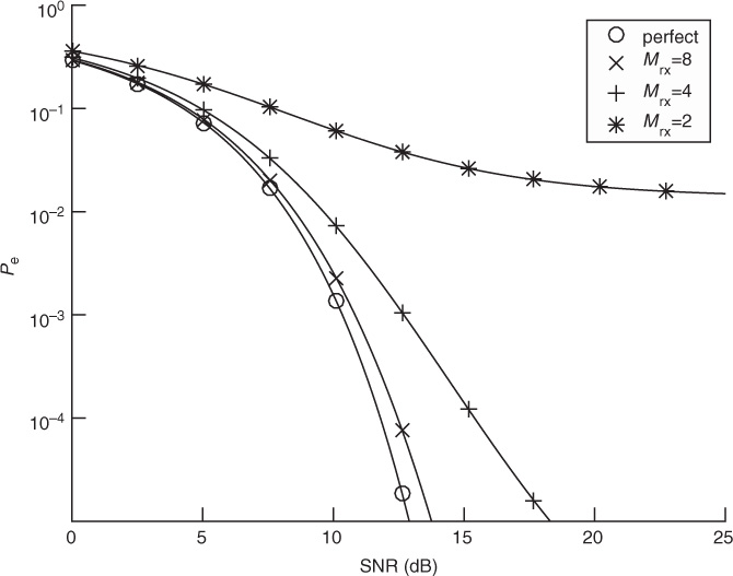
Figure 5.5 Plot of the exact symbol error rate for 4-QAM from (4.147), substituting SINR for SNR, with ![]() for different values of Mrx in (5.38), assuming a raised cosine pulse shape with α = 0.25. With enough oversampling, the effects of timing error are small.
for different values of Mrx in (5.38), assuming a raised cosine pulse shape with α = 0.25. With enough oversampling, the effects of timing error are small.
5.1.3 Frame Synchronization
The purpose of frame synchronization is to resolve multiple symbol period delays, assuming that symbol synchronization has already been performed. Let d denote the remaining offset where d = τd/T − k*/Mrx, assuming the symbol timing offset was corrected perfectly. Given that, ISI is eliminated and
To reconstruct the transmitted bit sequence it is necessary to know “where the symbol stream starts.” As with symbol synchronization, there is a great deal of theory surrounding frame synchronization [343, 224, 27]. This section considers one common algorithm for frame synchronization in flat channels that exploits the presence of a known training sequence, inserted during a training phase.
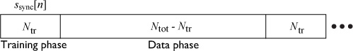
Most wireless systems insert reference signals into the transmitted waveform, which are known by the receiver. Known information is often called a training sequence or a pilot symbol, depending on how the known information is inserted. For example, a training sequence may be inserted at the beginning of a transmission as illustrated in Figure 5.6, or a few pilot symbols may be inserted periodically. Most systems use some combination of the two where long training sequences are inserted periodically and shorter training sequences (or pilot symbols) are inserted more frequently. For the purpose of explanation, it is assumed that the desired frame begins at discrete time n = 0. The total frame length is Ntot, including a length Ntr training phase and an Ntot − Ntr data phase. Suppose that ![]() is the training sequence known at the receiver.
is the training sequence known at the receiver.
One approach to performing frame synchronization is to correlate the received signal with the training sequence to compute
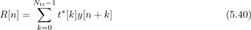
The maximization usually occurs by evaluating R[n] over a finite set of possible values. For example, the analog hardware may have a carrier sense feature that can determine when there is a significant signal of interest. Then the digital hardware can start evaluating the correlation and looking for the peak. A threshold can also be used to select the starting point, that is, finding the first value of n such that |R[n]| exceeds a target threshold. An example with frame synchronization is provided in Example 5.3.
Consider a system as described by (5.39) with ![]() , Ntr = 7, and Ntot = 21 with d = 0. We assume 4-QAM for the data transmission and that the training consists of the Barker code of length 7 given by
, Ntr = 7, and Ntot = 21 with d = 0. We assume 4-QAM for the data transmission and that the training consists of the Barker code of length 7 given by ![]() . The SNR is 5dB. We consider a frame snippet that consists of 14 data symbols, 7 training symbols, 14 data symbols, 7 training symbols, and 14 data symbols. In Figure 5.7, we plot |R[n]| computed from (5.40). There are two peaks that correspond to locations of our training data. The peaks happen at 21 and 42 as expected. If the snippet was delayed, then the peaks would shift accordingly.
. The SNR is 5dB. We consider a frame snippet that consists of 14 data symbols, 7 training symbols, 14 data symbols, 7 training symbols, and 14 data symbols. In Figure 5.7, we plot |R[n]| computed from (5.40). There are two peaks that correspond to locations of our training data. The peaks happen at 21 and 42 as expected. If the snippet was delayed, then the peaks would shift accordingly.

Figure 5.7 The absolute value of the output of a correlator for frame synchronization. The details of the simulation are provided in Example 5.3. Two correlation peaks are seen, corresponding to the location of the two training sequences.
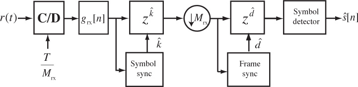
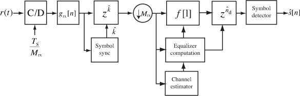
A block diagram of a receiver including both symbol synchronization and frame synchronization operations is illustrated in Figure 5.8. The frame synchronization happens after the downsampling and prior to the symbol detection. Fixing the frame synchronization requires advancing the signal by ![]() symbols.
symbols.
The frame synchronization algorithm may find a false peak if the data is the same as the training sequence. There are several approaches to avoid this problem. First, training sequences can be selected that have good correlation properties. There are many kinds of sequences known in the literature that have good autocorrelation properties [116, 250, 292], or periodic autocorrelation properties [70, 267]. Second, a longer training sequence may be used to reduce the likelihood of a false positive. Third, the training sequence can come from a different constellation than the data. This was used in Example 5.3 where a BPSK training sequence was used but the data was encoded with 4-QAM. Fourth, the frame synchronization can average over multiple training periods. Suppose that the training is inserted every Ntot symbols. Averaging over P periods then leads to an estimate

Larger amounts of averaging improve performance at the expense of higher complexity and more storage requirements. Finally, complementary training sequences can be used. In this case a pair of training sequences {t1[n]} and {t2[n]} are designed such that ![]() has a sharp correlation peak. Such sequences are discussed further in Section 5.3.1.
has a sharp correlation peak. Such sequences are discussed further in Section 5.3.1.
5.1.4 Channel Estimation
Once frame synchronization and symbol synchronization are completed, a good model for the received signal is
The two remaining impairments are the unknown flat channel h and the AWGN υ[n]. Because h rotates and scales the constellation, the channel must be estimated and either incorporated into the detection process or removed via equalization.
The area of channel estimation is rich and the history long [40, 196, 369]. In general, a channel estimation problem is handled like any other estimation problem. The formal approach is to derive an optimal estimator under assumptions about the signal and noise. Examples include the least squares estimator, the maximum likelihood estimator, and the MMSE estimator; background on these estimators may be found in Section 3.5.
In this section we emphasize the use of least squares estimation, which is also the ML estimator when used for linear parameter estimation in Gaussian noise. To use least squares, we build a received signal model from (5.43) by exploiting the presence of the known training sequence from n = 0, 1, . . . , Ntr − 1. Stacking the observations in (5.43) into vectors,

which becomes compactly
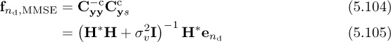
We already computed the maximum likelihood estimator for a more general version of (5.46) in Section 3.5.3. The solution was the least squares estimate, given by
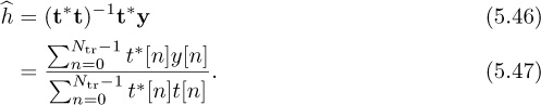
Essentially, the least squares estimator correlates the observed data with the training data and normalizes the result. The denominator is just the energy in the training sequence, which can be precomputed and stored offline. The numerator is calculated as part of the frame synchronization process. Therefore, frame synchronization and channel estimation can be performed jointly. The receiver, including symbol synchronization, frame synchronization, and channel estimation, is illustrated in Figure 5.9.
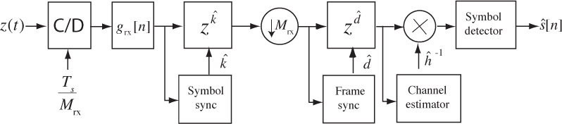
Figure 5.9 Receiver with symbol synchronization based on oversampling, frame synchronization, and channel estimation
In this example, we evaluate the squared error in the channel estimate. We consider a similar system to the one described in Example 5.3 with a length Ntr = 7 Barker code used for a training sequence, and a least squares channel estimator as in (5.46). We perform a Monte Carlo estimate of the channel by generating a noise realization and estimating the channel ![]() for n = 1, 2, . . . , 1000 realizations. In Figure 5.10, we evaluate the estimation error as a function of the SNR, which is defined as
for n = 1, 2, . . . , 1000 realizations. In Figure 5.10, we evaluate the estimation error as a function of the SNR, which is defined as ![]() , and is 5dB in this example. We plot the error for one realization of a channel estimation, which is given by
, and is 5dB in this example. We plot the error for one realization of a channel estimation, which is given by ![]() , and the mean squared error, which is given by
, and the mean squared error, which is given by ![]() . The plot shows how the estimation error, based both on one realization and on average, decreases with SNR.
. The plot shows how the estimation error, based both on one realization and on average, decreases with SNR.
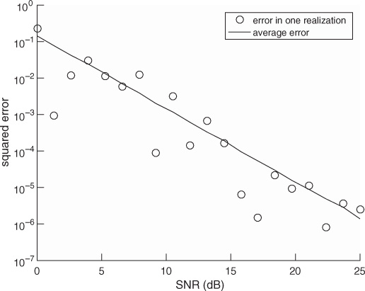
Figure 5.10 Estimation error as a function of SNR for the system in Example 5.4. The error estimate reduces as SNR increases.
In this example, we evaluate the squared error in the channel estimate for different lengths of 4-QAM training sequences, an SNR of 5dB, the channel as in Example 5.3, and a least squares channel estimator as in (5.46). We perform a Monte Carlo estimate of the squared error of one realization and the mean squared error, as described in Example 5.4. We plot the results in Figure 5.11, which show how longer training sequences reduce estimation error. Effectively, longer training increases the effective SNR through the addition of energy through coherent combining in ![]() and more averaging in
and more averaging in ![]() .
.
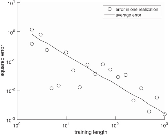
Figure 5.11 Estimation error as a function of the training length for the system in Example 5.5. The error estimate reduces as the training length increases.
5.1.5 Equalization
Assuming that channel estimation has been completed, the next step in the receiver processing is to use the channel estimate to perform symbol detection. There are two reasonable approaches; both involve assuming that ![]() is the true channel estimate. This is a reasonable assumption if the channel estimation error is small enough.
is the true channel estimate. This is a reasonable assumption if the channel estimation error is small enough.
The first approach is to incorporate ![]() into the detection process. Replacing
into the detection process. Replacing ![]() by h in (4.105), then
by h in (4.105), then
Consequently, the channel estimate becomes an input into the detector. It can be used as in (5.48) to scale the symbols during the computation of the norm, or it can be used to create a new constellation ![]() and detection performed using the scaled constellation as
and detection performed using the scaled constellation as
The latter approach is useful when Ntot is large.
An alternative approach to incorporating the channel into the ML detector is to remove the effects of the channel prior to detection. For ![]() ,
,

The process of creating the signal ![]() is an example of equalization. When equalization is used, the effects of the channel are removed from y[n] and a standard detector can be applied to the result, leveraging constellation symmetries to reduce complexity. The receiver, including symbol synchronization, frame synchronization, channel estimation, and equalization, is illustrated in Figure 5.9.
is an example of equalization. When equalization is used, the effects of the channel are removed from y[n] and a standard detector can be applied to the result, leveraging constellation symmetries to reduce complexity. The receiver, including symbol synchronization, frame synchronization, channel estimation, and equalization, is illustrated in Figure 5.9.
The probability of symbol error with channel estimation can be computed by treating the estimation error as noise. Let ![]() where
where ![]() is the estimation error. For a given channel h and estimate
is the estimation error. For a given channel h and estimate ![]() the equalized received signal is
the equalized received signal is

It is common to treat the middle interference term as additional noise. Moving the common ![]() to the numerator,
to the numerator,

This can be used as part of a Monte Carlo simulation to determine the impact of channel estimation. Since the receiver does not actually know the estimation error, it is also common to consider a variation of the SINR expression where the variance of the estimate ![]() is used in place of the instantaneous value (assuming that the estimator is unbiased so zero mean). Then the SINR becomes
is used in place of the instantaneous value (assuming that the estimator is unbiased so zero mean). Then the SINR becomes

This expression can be used to study the impact of estimation error on the probability of error, as the mean squared error of the estimate is a commonly computed quantity. A comparison of the probability of symbol error for these approaches is provided in Example 5.6.
In this example we evaluate the impact of channel estimation error. We consider a system similar to the one described in Example 5.4 with a length Ntr = 7 Barker code used for a training sequence, and a least squares channel estimator as in (5.46). We perform a Monte Carlo estimate of the channel by generating a noise realization and estimating the channel ![]() for n = 1, 2, . . . , 1000 realizations. For each realization, we compute the error, insert into the
for n = 1, 2, . . . , 1000 realizations. For each realization, we compute the error, insert into the ![]() in (5.53), and use that to compute the exact probability of symbol error from Section 4.4.5. We then average this over 1000 Monte Carlo simulations. We also compare in Figure 5.12 with the probability of error assuming no estimation error with SNR |h|2Ex/No and with the probability of error computed using the average error from the SINR in (5.54). We see in this example that the loss due to estimation error is about 1dB and that there is little difference in the average probability of symbol error and the probability of symbol error computed using the average estimation error.
in (5.53), and use that to compute the exact probability of symbol error from Section 4.4.5. We then average this over 1000 Monte Carlo simulations. We also compare in Figure 5.12 with the probability of error assuming no estimation error with SNR |h|2Ex/No and with the probability of error computed using the average error from the SINR in (5.54). We see in this example that the loss due to estimation error is about 1dB and that there is little difference in the average probability of symbol error and the probability of symbol error computed using the average estimation error.
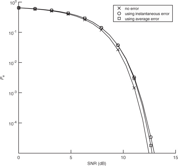
Figure 5.12 The probability of symbol error with 4-QAM and channel estimation using a length Ntr = 7 training sequence. The probability of symbol error with no channel estimation error is compared with the average of the probability of symbol error including the instantaneous error, and the probability of symbol error using the average estimation error. There is little loss in using the average estimation error.
5.1.6 Carrier Frequency Offset Synchronization
Wireless communication systems use passband communication signals. They can be created at the transmitter by upconverting a complex baseband signal to carrier fc and can be processed at the receiver to produce a complex baseband signal by downconverting from a carrier fc. In Section 3.3, the process of upconversion to carrier fc, downconversion to baseband, and the complex equivalent notation were explained under the important assumption that fc is known perfectly at both the transmitter and the receiver. In practice, fc is generated from a local oscillator. Because of temperature variations and the fact that the carrier frequency is generated by a different local oscillator and transmitter and receiver, in practice fc at the transmitter is not equal to ![]() at the receiver as illustrated in Figure 5.13. The difference between the transmitter and the receiver
at the receiver as illustrated in Figure 5.13. The difference between the transmitter and the receiver ![]() is the carrier frequency offset (or simply frequency offset) and is generally measured in hertz. In device specification sheets, the offset is often measured as |fe|/fc and is given in units of parts per million. In this section, we derive the system model for carrier frequency offset and present a simple algorithm for carrier frequency offset estimation and correction.
is the carrier frequency offset (or simply frequency offset) and is generally measured in hertz. In device specification sheets, the offset is often measured as |fe|/fc and is given in units of parts per million. In this section, we derive the system model for carrier frequency offset and present a simple algorithm for carrier frequency offset estimation and correction.
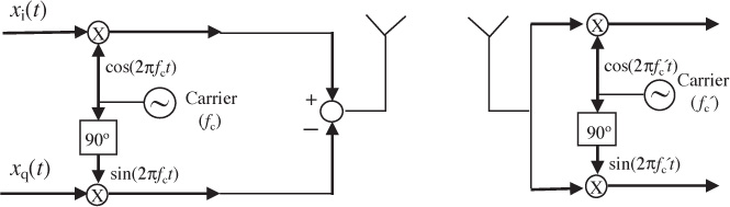
Figure 5.13 Abstract block diagram of a wireless system with different carrier frequencies at the transmitter and the receiver
Let
be the passband signal generated at the transmitter. Let the observed passband signal at the receiver at carrier fc be
where r(t) = ri(t) + jrq(t) is the complex baseband signal that corresponds to rp(t) and we use the fact that ![]() for the last step. Now suppose that rp(t) is downconverted using carrier
for the last step. Now suppose that rp(t) is downconverted using carrier ![]() to produce a new signal r′(t). Then the extracted complex baseband signal is (ignoring noise)
to produce a new signal r′(t). Then the extracted complex baseband signal is (ignoring noise)
Focusing on the last term in (5.59) with ![]() , then
, then

Substituting in rp(t) from (5.58),
Lowpass filtering (assuming, strictly speaking, a bandwidth of B + |fe|) and correcting for the factor of ![]() leaves the complex baseband equivalent
leaves the complex baseband equivalent
Carrier frequency offset results in a rolling phase shift that happens after the convolution and depends on the difference in carrier fe. As the phase shift accumulates, failing to synchronize can quickly lead to errors.
Following the methodology of this book, it is of interest to formulate and solve the frequency offset estimation and correction problem purely in discrete time. To that end a discrete-time complex baseband equivalent model is required.
To formulate a discrete-time model, we focus on the sampled signal after matched filtering, still neglecting noise, as

Suppose that the frequency offset fe is sufficiently small that the variation over the duration of grx(t) can be assumed to be a constant; then e−j2πfeτgrx(τ) ≈ grx(τ). This is reasonable since most of the energy in the matched filter grx(t) is typically concentrated over a few symbol periods. Assuming this holds,
As a result, it is reasonable to model the effects of frequency offset as if they occurred on the matched filtered signal.
Now we specialize to the case of flat-fading channels. Substituting for r(t), adding noise, and sampling gives

where ![]() = feT is the normalized frequency offset. Frequency offset introduces a multiplication by the discrete-time complex exponential ej2πfeTn.
= feT is the normalized frequency offset. Frequency offset introduces a multiplication by the discrete-time complex exponential ej2πfeTn.
To visualize the effects of frequency offset, suppose that symbol and frame synchronization has been accomplished and only equalization and channel estimation remain. Then the Nyquist property of the pulse shape can be exploited so that
Notice that the transmit symbol is being rotated by exp(j2π![]() n). As n increases, the offset increases, and thus the symbol constellation rotates even further. The impact of this is an increase in the number of symbol errors as the symbols rotate out of their respective Voronoi regions. The effect is illustrated in Example 5.7.
n). As n increases, the offset increases, and thus the symbol constellation rotates even further. The impact of this is an increase in the number of symbol errors as the symbols rotate out of their respective Voronoi regions. The effect is illustrated in Example 5.7.
Consider a system with the frequency offset described by (5.69). Suppose that ![]() = 0.05. In Figure 5.14, we plot a 4-QAM constellation at times n = 0, 1, 2, 3. The Voronoi regions corresponding to the unrotated constellation are shown on each plot as well. To make seeing the effect of the rotation easier, one point is marked with an x. Notice how the rotations are cumulative and eventually the constellation points completely leave their Voronoi regions, which results in detection errors even in the absence of noise.
= 0.05. In Figure 5.14, we plot a 4-QAM constellation at times n = 0, 1, 2, 3. The Voronoi regions corresponding to the unrotated constellation are shown on each plot as well. To make seeing the effect of the rotation easier, one point is marked with an x. Notice how the rotations are cumulative and eventually the constellation points completely leave their Voronoi regions, which results in detection errors even in the absence of noise.

Figure 5.14 The successive rotation of a 4-QAM constellation due to frequency offset. The Voronoi regions for each constellation point are indicated with the dashed lines. To make the effects of the rotation clearer, one of the constellation points is marked with an x.
Correcting for frequency offset is simple: just multiply y[n] by e−j2π![]() n. Unfortunately, the offset is unknown at the receiver. The process of correcting for
n. Unfortunately, the offset is unknown at the receiver. The process of correcting for ![]() is known as frequency offset synchronization. The typical method for frequency offset synchronization involves first estimating the offset
is known as frequency offset synchronization. The typical method for frequency offset synchronization involves first estimating the offset ![]() , then correcting for it by forming the new sequence
, then correcting for it by forming the new sequence ![]() with the phase removed. There are several different methods for correction; most employ a frequency offset estimator followed by a correction phase. Blind offset estimators use some general properties of the received signal to estimate the offset, whereas non-blind estimators use more specific properties of the training sequence.
with the phase removed. There are several different methods for correction; most employ a frequency offset estimator followed by a correction phase. Blind offset estimators use some general properties of the received signal to estimate the offset, whereas non-blind estimators use more specific properties of the training sequence.
Now we review two algorithms for correcting the frequency offset in a flat-fading channel. We start by observing that frequency offset does not impact symbol synchronization, since the ej2πfeTn cancels out the maximum output energy maximization caused by the magnitude function (see, for example, (5.15)). As a result, ISI cancels and a good model for the received signal is
where the offset ![]() , the channel h, and the frame offset d are unknowns. In Example 5.8, we present an estimator based on a specific training sequence design. In Example 5.9, we use properties of 4-QAM to develop a blind frequency offset estimator. We compare their performance to highlight differences in the proposed approaches in Figure 5.15. We also explain how to jointly estimate the delay and channel with each approach. These algorithms illustrate some ways that known information or signal structure can be exploited for estimation.
, the channel h, and the frame offset d are unknowns. In Example 5.8, we present an estimator based on a specific training sequence design. In Example 5.9, we use properties of 4-QAM to develop a blind frequency offset estimator. We compare their performance to highlight differences in the proposed approaches in Figure 5.15. We also explain how to jointly estimate the delay and channel with each approach. These algorithms illustrate some ways that known information or signal structure can be exploited for estimation.

Figure 5.15 The mean squared error performance of two different frequency offset estimators: the training-based approach in Example 5.8 and the blind approach in Example 5.9. Frame synchronization is assumed to have been performed already for the coherent approach. The channel is the same as in Example 5.3 and other examples, and the SNR is 5dB. The true frequency offset is ![]() = 0.01. The estimators are compared assuming the number of samples (Ntr for the coherent case and Ntot for the blind case). The error in each Monte Carlo simulation is computed from phase
= 0.01. The estimators are compared assuming the number of samples (Ntr for the coherent case and Ntot for the blind case). The error in each Monte Carlo simulation is computed from phase ![]() to avoid any phase wrapping effects.
to avoid any phase wrapping effects.
In this example, we present a coherent frequency offset estimator that exploits training data. We suppose that frame synchronization has been solved. Let us choose as a training sequence t[n] = exp(j2πftn) for n = 0, 1, . . . , Ntr − 1 where ft is a fixed frequency. This kind of structure is available from the Frequency Correction Burst in GSM, for example [100]. Then for n = 0, 1, . . . , Ntr − 1,
Correcting the known offset introduced by the training data gives
The rotation by e−j2πftn does not affect the distribution of the noise. Solving for the unknown frequency in (5.72) is a classic problem in signal processing and single-tone parameter estimation, and there are many approaches [330, 3, 109, 174, 212, 218]. We explain the approach used in [174] based on the model in [330]. Approximate the corrected signal in (5.72) as
where θ is the phase of h and ν[n] is Gaussian noise. Then, looking at the phase difference between two adjacent samples, a linear system can be written from the approximate model as
Aggregating the observations in (5.79) from n = 1, . . . , Ntot − 1, we can create a linear estimation problem
where [p]n = phase(ej2πftny*[n]e−j2πft(n+1)y[n + 1]), 1 is an Ntr − 1 × 1 vector, and ν is an Ntr − 1 × 1 noise vector. The least squares solution is given by

which is also the maximum likelihood solution if ν[n] is assumed to be IID [174].
Frame synchronization and channel estimation can be incorporated into this estimator as follows. Given that the frequency offset estimator in (5.77) solves a least squares problem, there is a corresponding expression for the squared error; see, for example, (3.426). Evaluate this expression for many possible delays and choose the delay that has the lowest squared error. Correct for the offset and delay, then estimate the channel as in Section 5.1.4.
In this example, we exploit symmetry in the 4-QAM constellation to develop a blind frequency offset estimator, which does not require training data. The main observation is that for 4-QAM, the normalized constellation symbols are points on the unit circle. In particular for 4-QAM, it turns out that s4[n] = −1. Taking the fourth power,
where ν[n] contains noise and products of the signal and noise. The unknown parameter d disappears because s4[n − d] = −1, assuming a continuous stream of symbols. The resulting equation has the form of a complex sinusoid in noise, with unknown frequency, amplitude, and phase similar to (5.72). Then a set of linear equations can be written from
in a similar fashion to (5.75), and then

Frame synchronization and channel estimation can be incorporated as follows. Use all the data to estimate the carrier frequency offset from (5.80). Then correct for the offset and perform frame synchronization and channel estimation based on training data, as outlined in Section 5.1.3 and Section 5.1.4.
5.2 Equalization of Frequency-Selective Channels
In this and subsequent sections, we generalize the development in Section 5.1 to frequency-selective fading channels. We focus specifically on equalization, assuming that channel estimation, frame synchronization, and frequency offset synchronization have been performed. We solve the channel estimation problem in Section 5.3 and the frame and frequency offset synchronization problems in Section 5.4. First we develop the discrete-time received signal model, including a frequency-selective channel and AWGN. Then we develop three approaches for linear equalization. The first approach is based on constructing an FIR filter that approximately inverts the effective channel. The second approach is to insert a special prefix in the transmitted signal to permit frequency-domain equalization at the receiver, in what is called SC-FDE. The third approach also uses a cyclic prefix but precodes the information in the frequency domain, in what is called OFDM modulation. As the equalization removes intersymbol interference, standard symbol detection follows the equalization operations.
5.2.1 Discrete-Time Model for Frequency-Selective Fading
In this section, we develop a received signal model for general frequency-selective channels, generalizing the results for a single path in Section 5.1.1. Assuming perfect synchronization, the received complex baseband signal after matched filtering but prior to sampling is
Essentially, y(t) takes the form of a complex pulse-amplitude modulated signal but where g(t) is replaced by ![]() . Except in special cases, this new effective pulse is no longer a Nyquist pulse shape.
. Except in special cases, this new effective pulse is no longer a Nyquist pulse shape.
We now develop a sampled signal model. Let
denote the sampled effective discrete-time channel. This channel combines the complex baseband equivalent model of the propagation channel, the transmit pulse-shaping filter, the receive pulse matched transmit filter, and the scaled transmit energy ![]() .
.
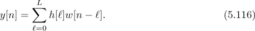
Sampling (5.82) at the symbol rate and with the effective discrete-time channel gives the received signal
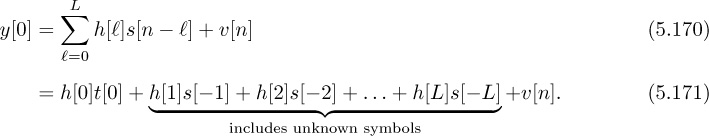
The main distortion is ISI, since every observation y[n] is a linear combination of all the transmitted symbols through the convolution integral.
To get some insight into the impact of intersymbol interference, suppose that ![]() . Then
. Then
The nth symbol s[n] is subject to interference from s[n − 1], sent in the previous symbol period. Without correcting for this interference, detection performance will be bad. Treating ISI as noise,
For example, for SNR = 10dB = 10 and |h1|2 = 1, SINR = 10/(10+1) = 0.91 or −0.4dB. Figure 5.16 shows the SINR as a function of |h1|2 for SNR = 10dB and SNR = 5dB.
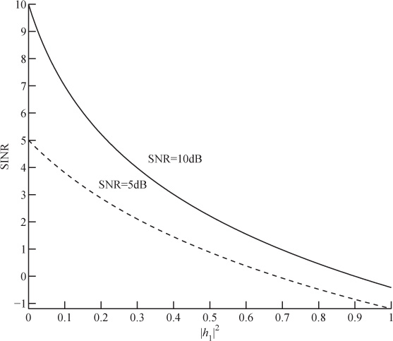
Figure 5.16 The SINR as a function of |h1|2 for the discrete-time channel ![]() in Example 5.10.
in Example 5.10.
To develop receiver signal processing algorithms, it is reasonable to treat h[n] as causal and FIR. The causal assumption is reasonable because the propagation channel cannot predict the future. Furthermore, frame synchronization algorithms attempt to align, assuming a causal impulse response. The FIR assumption is reasonable because (a) there are no perfectly reflecting environments and (b) the signal energy decays as a function of distance between the transmitter and the receiver. Essentially, every time the signal reflects, some of the energy passes through the reflector or is scattered and thus it loses energy. As the signal propagates, it also loses power as it spreads in the environment. Multipaths that are weak will fall below the noise threshold. With the FIR assumption,
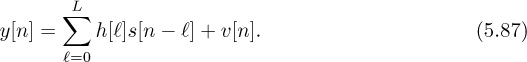
The channel is fully specified by the L+1 coefficients ![]() . The order of the channel, given by L, determines to a large extent the severity of the ISI. Flat fading corresponds to the special case of L = 0. We develop equalizers specifically for the system model in (5.87), assuming that the channel coefficients are perfectly known at the receiver.
. The order of the channel, given by L, determines to a large extent the severity of the ISI. Flat fading corresponds to the special case of L = 0. We develop equalizers specifically for the system model in (5.87), assuming that the channel coefficients are perfectly known at the receiver.
5.2.2 Linear Equalizers in the Time Domain
In this section, we develop an FIR equalizer to remove (approximately) the effects of ISI. We suppose that the channel coefficients are known perfectly; they can be estimated using training data via the method described in Section 5.3.1.
There are many strategies for equalization. One of the best approaches is to apply what is known as maximum likelihood sequence detection [348]. This is a generalization of the AWGN detection rule, which incorporates the memory in the channel due to L > 0. Unfortunately, this detector is complex to implement for channels with large L, though note that it is implemented in practical systems for modest values of L. Another approach is decision feedback equalization, where the contributions of detected symbols are subtracted, reducing the extent of the ISI [17, 30]. Combinations of these approaches are also possible.
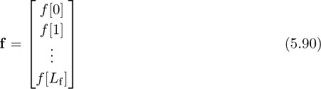
In this section, we develop an FIR linear equalizer that operates on the time-domain signal. The goal of a linear equalizer is to find a filter that removes the effects of the channel. Let ![]() be an FIR equalizer. The length of the equalizer is given by Lf. The equalizer is also associated with an equalizer delay nd, which is a design parameter. Generally, allowing nd > 0 improves performance. The best equalizers consider several values of nd and choose the best one.
be an FIR equalizer. The length of the equalizer is given by Lf. The equalizer is also associated with an equalizer delay nd, which is a design parameter. Generally, allowing nd > 0 improves performance. The best equalizers consider several values of nd and choose the best one.
An ideal equalizer, neglecting noise, would satisfy

for n = 0, 1, . . . , Lf + L. Unfortunately, there are only Lf + 1 unknown parameters, so (5.88) can be satisfied exactly only in trivial cases like flat fading. This is not a surprise, as we know from DSP that the inverse of an FIR filter is an IIR filter. Alternatively, we pursue a least squares solution to (5.88).
We write (5.88) as a linear system and then find the least squares solution. The key idea is to write a set of linear equations and solve for the filter coefficients that ensure that (5.88) minimizes the squared error. First incorporate the channel coefficients into the Lf + L + 1 × Lf + 1 convolution matrix:

Then write the equalizer coefficients in a vector
and the desired response as the vector end with zeros everywhere except for a 1 in the nd + 1 position. With these definitions, the desired linear system is
The least squares solution is
with squared error
The squared error can be minimized further by choosing nd such that J[nd] is minimized. This is known as optimizing the equalizer delay.
In this example, we compute the least squares optimal equalizer of length Lf = 6 for a channel with impulse response h[0] = 0.5, h[1] = j/2, and h[2] = 0.4 exp(j * π/5). First we construct the convolution matrix
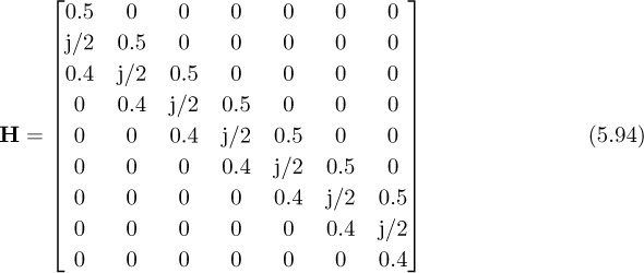
and use it to compute (5.93) to determine the optimal equalizer length. As illustrated in Figure 5.17(a), the optimum delay occurs at nd = 5 with J[5] = 0.0266. The optimum equalizer derived from (5.92) is
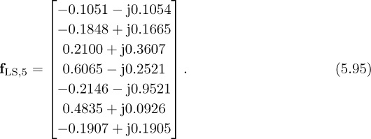
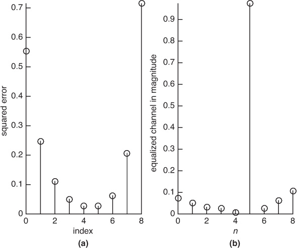
Figure 5.17 The squared error for the equalizer J[nd] in (a) and the equalized channel h[n] * fnd[n] in (b), corresponding to the parameters in Example 5.11
The equalized impulse response is plotted in Figure 5.17(b).
The matrix H has a special kind of structure. Notice that the diagonals are all constant. This is known as a Toeplitz matrix, sometimes called a filtering matrix. It shows up often when writing a convolution in matrix form. The structure in Toeplitz matrices also leads to many efficient algorithms for solving least squares equations, implementing adaptive solutions, and so on [172, 294]. This structure also means that H is full rank as long as at least one coefficient is nonzero. Therefore, the inverse in (5.92) exists.
The equalizer is applied to the sampled received signal to produce
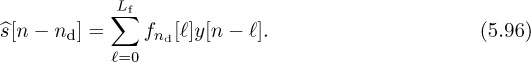
The delay nd is known and can be corrected by advancing the output by the corresponding number of samples.
An alternative to the least squares equalizer is the LMMSE equalizer. Let us rewrite (5.96) to place the equalizer coefficients into a single vector
where yT[n] = [y[n], y[n − 1], . . . , y[n − Lf]T,
with sT[n] = [s[n], s[n − 1], . . . , s[n − L]]T and H as in (5.89). We seek the equalizer that minimizes the mean squared error
Assume that s[n] is IID with zero mean and unit variance, v[n] is IID with variance ![]() , and s[n] and v[n] are independent. As a result,
, and s[n] and v[n] are independent. As a result,
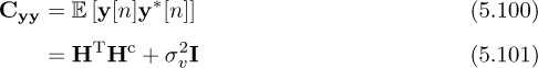

Then we can apply the results from Section 3.5.4 to derive
where the conjugate results from the use of conjugate transpose in the formulation of the equalizer in (3.459). The LMMSE equalizer gives an inverse that is regularized by the noise power ![]() , which is No if the only impairment is AWGN. This should improve performance at lower values of the SNR where equalization creates the most noise enhancement.
, which is No if the only impairment is AWGN. This should improve performance at lower values of the SNR where equalization creates the most noise enhancement.
The asymptotic equalizer properties are interesting. As ![]() , fnd,MMSE → fLS,nd. In the absence of noise, the MMSE solution becomes the LS solution. As
, fnd,MMSE → fLS,nd. In the absence of noise, the MMSE solution becomes the LS solution. As ![]() ,
, ![]() . This can be seen as a spatially matched filter.
. This can be seen as a spatially matched filter.
A block diagram of linear equalization and channel estimation is illustrated in Figure 5.18. Note that the optimization over delay and correction for delay are included in the equalization computation, though they could be separated in additional blocks. Symbol synchronization is included in the diagram, despite the fact that linear equalization can correct for symbol timing errors through equalization. The reason is that SNR performance can nonetheless be improved by taking the best sample, especially when the pulse shape has excess bandwidth. An alternative is to implement a fractionally spaced equalizer, which operates on the signal prior to downsampling [128]. This is explored further in the problems at the end of the chapter.
A final comment on complexity. The length of the equalizer Lf is a design parameter that depends on L. The parameter L is the extent of the multipath in the channel and is determined by the bandwidth of the signal as well as the maximum delay spread derived from propagation channel measurements. The equalizer is an approximate FIR inverse of an FIR filter. As a consequence, performance will improve if Lf is large, assuming perfect channel knowledge. The complexity required per symbol, however, also grows with Lf. Thus there is a trade-off between choosing large Lf to have better equalizer performance and smaller Lf to have more efficient receiver implementation. A rule of thumb is to take Lf to be at least 4L.
5.2.3 Linear Equalization in the Frequency Domain with SC-FDE
Both the direct and the indirect equalizers require a convolution on the received signal to remove the effects of the channel. In practice this can be done with a direct implementation using the overlap-and-add or overlap-and-save methods for efficiently computing convolutions in the frequency domain. An alternative to FIR in the time domain is to perform equalization completely in the frequency domain. This has the advantage of allowing an ideal inverse of the channel to be computed. Application of frequency-domain equalization, though, requires additional mathematical structure in the transmitted waveform as we now explain.
In this section, we describe a technique known as SC-FDE [102]. At the transmitter, SC-FDE divides the symbols into blocks and adds redundancy in the form of a cyclic prefix. The receiver can exploit this extra information to permit equalization using the DFT. The result is an equalization strategy that is capable of perfectly equalizing the channel, in the absence of noise. SC-FDE is supported in IEEE 802.11ad, and a variation is used in the uplink of 3GPP LTE.
We now explain the motivation for working with the DFT and the key ideas behind the cyclic prefix. First, we explain why direct application of the DTFT is not feasible. Consider the received signal with intersymbol interference but without noise in (5.87). In the frequency domain
The ideal zero-forcing equalizer is
Unfortunately, it is not possible to directly implement the ideal zero-forcing equalizer in the DTFT frequency domain. First of all, the equalizer does not exist at f for which H(ej2πf) is zero. This can be solved by using a pseudo-inverse rather than an inverse equalizer. Several more important problems occur as a by-product of the use of the DTFT. It is often not possible to compute the ideal DTFT in practice. For example, the whole {s[n]} → S(ej2πf) is required, but typically only a few samples of s[n] are available. Even when {s[n]} is available, the DTFT may not even exist since the sum may not converge. Furthermore, it is not possible to observe over a long interval since h[ℓ] is time invariant only over a short window.
A solution to this problem is to use a specially designed {s[n]} and leverage the principles of the discrete Fourier transform. A comprehensive discussion of the DFT and its properties is provided in Chapter 3. To review, recall that the DFT is a basis expansion for finite-length signals:

The DFT can be computed efficiently with the FFT for N as a power of 2 and certain other special cases. Practical implementations of the DFT use the FFT. The key properties of the DFT are summarized in Table 3.5.
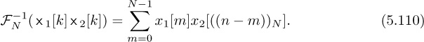
A distinguishing feature of the DFT is that multiplication in frequency corresponds to circular convolution in time. Consider two sequences ![]() and
and ![]() . Let FN (·) denote the DFT operation on a length N signal, and let
. Let FN (·) denote the DFT operation on a length N signal, and let ![]() denote its inverse. With ×1[k] = FN (x1[n]) and ×2[k] = FN [x2[n]], then
denote its inverse. With ×1[k] = FN (x1[n]) and ×2[k] = FN [x2[n]], then
Unfortunately, linear convolution, not circular convolution, is a good model for the effects of wireless propagation per (5.87).
It is possible to mimic the effects of circular convolution by modifying the transmitted signal with a suitably chosen guard interval. The most common choice is what is called a cyclic prefix, illustrated in Figure 5.19. To understand the need for a cyclic prefix, consider the circular convolution between a block of symbols of length N where N > L: ![]() and the channel
and the channel ![]() , which has been zero padded to have length N, that is, h[n] = 0 for n ∈ [L + 1, N − 1]. The output of the circular convolution is
, which has been zero padded to have length N, that is, h[n] = 0 for n ∈ [L + 1, N − 1]. The output of the circular convolution is


The portion for n ≥ L looks like a linear convolution; the circular wrap-around occurs only for the first L samples.
Now we modify the transmitted sequence to obtain a circular convolution from the linear convolution introduced by the channel. Let Lc ≥ L be the length of the cyclic prefix. Form the signal ![]() where the cyclic prefix is
where the cyclic prefix is
After convolution with an L + 1 tap channel, and neglecting noise for the derivation,
Now we neglect the first Lc terms of the convolution, which is called discarding the cyclic prefix, to form the new signal:

To see the effect, it is useful to evaluate ![]() for a few values of n:
for a few values of n:
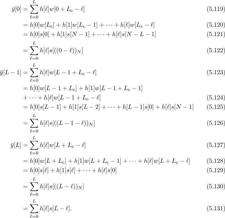
For values of n < L, the cyclic prefix replicates the effects of the linear convolution observed in (5.113). For values of N ≥ L, the circular convolution becomes a linear convolution, also as expected from (5.113) because L < N. In general, the truncated sequence satisfies
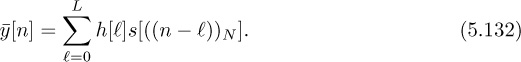
Therefore, thanks to the cyclic prefix, it is possible to implement frequency-domain equalization simply by computing ![]() ,
, s[k] = FN (s[n]), and then

This is the key idea behind the SC-FDE equalizer.
The cyclic prefix also acts as a guard interval, separating the contributions of different blocks of data. To see this, note that ![]() depends only on symbols
depends only on symbols ![]() and not symbols sent in previous blocks like s[n] for n < 0 or n > N. Zero padding can alternatively be used as a guard interval, as explored in Example 5.12.
and not symbols sent in previous blocks like s[n] for n < 0 or n > N. Zero padding can alternatively be used as a guard interval, as explored in Example 5.12.
Zero padding is an alternative to the cyclic prefix [236]. With zero padding, Lc zero values replace the cyclic prefix where
The data is encoded as in (5.115) and L ≤ Lc. We neglect noise for this problem.
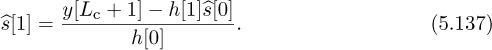
• Show how zero padding enables successive decoding of s[n] from y[n]. Hint: Start with n = 0 and show that s[0] can be derived from y[Lc]. Let ![]() denote the detected symbol. Then show how, by subtracting off
denote the detected symbol. Then show how, by subtracting off ![]() , you can detect
, you can detect ![]() . Then assume it is true for a given n and show that it works for n + 1.
. Then assume it is true for a given n and show that it works for n + 1.
Answer: To decode s[0], we look at the expression of y[Lc]. After expanding and simplifying, because of the zeros, we obtain y[Lc] = h[0]w[Lc] = h[0]s[0]. Because h[0] is known, we can decode s[0] as
To decode s[1], we use y[Lc + 1] and the previously detected value of ![]() . Because
. Because ![]() , and assuming the detected symbol is correct,
, and assuming the detected symbol is correct,
Finally, assume that ![]() has been decoded; then
has been decoded; then

We thus can decode s[k] as follows:
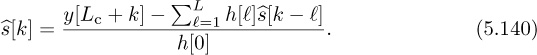
The main drawback of this approach is that it suffers from error propagation: a symbol error in ![]() affects the detection of all symbols after k.
affects the detection of all symbols after k.
• Consider the following alternative to discarding the cyclic prefix:

Show how this structure also permits frequency domain equalization (neglect noise for the derivation).
Answer: For n = 0, 1, . . . , L − 1:

where the cancellation is due to the cyclic prefix. For n = L, L − 1, . . . , N − 1:

Therefore, ![]() is the same as (5.132), and the same equalization as SC-FDE can be applied, with a little performance penalty due to the double addition of noise. Zero padding has been used in UWB (ultra-wideband) [197] to make multiband OFDM easier to implement, and in millimeter-wave SC-FDE systems [82], where it allows for reconfiguration of the RF parameters without signal distortion.
is the same as (5.132), and the same equalization as SC-FDE can be applied, with a little performance penalty due to the double addition of noise. Zero padding has been used in UWB (ultra-wideband) [197] to make multiband OFDM easier to implement, and in millimeter-wave SC-FDE systems [82], where it allows for reconfiguration of the RF parameters without signal distortion.
Noise has an adverse effect on the performance of the SC-FDE equalizer. Now we examine what happens to the effective noise variance after equalization. In the presence of noise, and with perfect channel state information,
The second term is augmented during the equalization process in what is called noise enhancement. Let ![]() be the enhanced noise component. It remains zero mean. To compute its variance, we expand the enhanced noise as
be the enhanced noise component. It remains zero mean. To compute its variance, we expand the enhanced noise as
and then compute
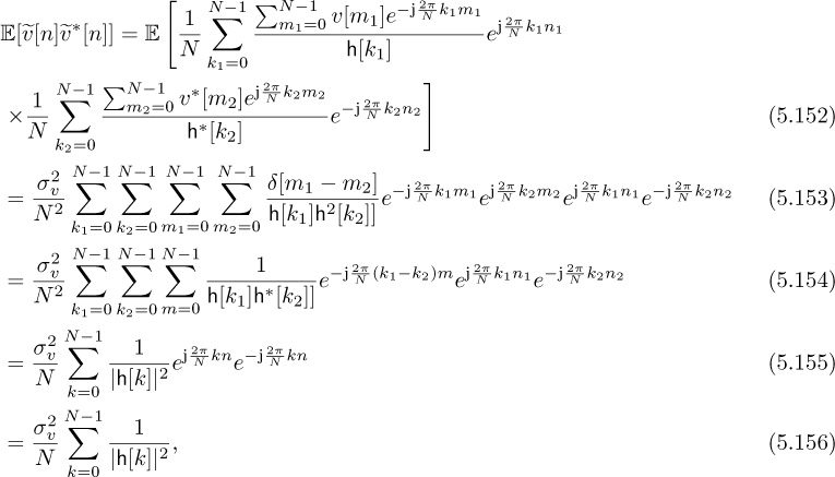
where the results follow from the IID property of υ[n] and repeated applications of the orthogonality of discrete-time complex exponentials. The main conclusion is that we can model (5.150) as
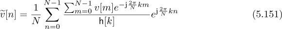
where ν[n] is AWGN with variance given in (5.156), which is the geometric mean of the inverse of the channel in the frequency domain. We contrast this result with that obtained using OFDM in the next section.
An implementation of a QAM system with frequency-domain equalization is illustrated in Figure 5.20. The operation of collecting the input bits into groups of N symbols is given by the serial-to-parallel converter. A cyclic prefix takes the N input symbols, copies the last Lc symbols to the beginning, and outputs N + Lc symbols. The resulting symbols are then converted from parallel to serial, followed by upsampling and the usual matched filtering. The serial-to-parallel and parallel-to-serial blocks can be implemented from a DSP perspective using simple filter banks.
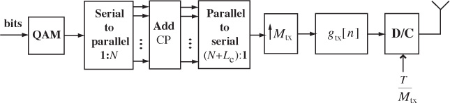
Figure 5.20 QAM transmitter for a single-carrier frequency-domain equalizer, with CP denoting cyclic prefix
Compared with linear equalization, SC-FDE has several advantages. The channel inverse can be done perfectly since the inverse is exact in the DFT domain (assuming, of course, that none of the h[k] are zero), and the time-domain equalizer is an approximate inverse. SC-FDE also works regardless of the value of L as long as Lc ≥ L. The equalizer complexity is fixed and is determined by the complexity of the FFT operation, proportional to N log2 N. The complexity of the time-domain equalizer is a function of K and generally grows with L (assuming that K grows with L), unless it is itself implemented in the frequency domain. As a general rule of thumb it becomes more efficient to equalize in the frequency domain for L around 5.
The main parameters to select in SC-FDE are N and Lc. To minimize complexity it makes sense to take N to be small. The amount of overhead, though, is Lc/(N + Lc). Consequently, taking N to be large reduces the system overhead incurred by redundancy in the cyclic prefix. Too large an N, however, may mean that the channel varies over the N symbols, violating the LTI assumption. In general, Lc is selected to be large enough that L < Lc for most channel realizations, throughout the use cases of the wireless system. For example, for a personal area network application, indoor channel measurements may be used to establish the power delay profile and other channel statistics from which a maximum value of Lc can be derived.
5.2.4 Linear Equalization in the Frequency Domain with OFDM
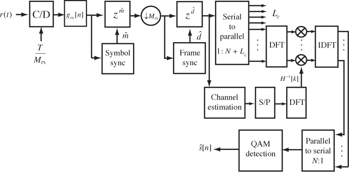
The SC-FDE receiver illustrated in Figure 5.21 performs a DFT on a portion of the received signal, equalizes with the DFT of the channel, and takes the IDFT (inverse discrete Fourier transform) to form the equalized sequence ![]() . This offloads the primary equalization operations to the receiver. In some cases, however, it is of interest to have a more balanced load between transmitter and receiver. A solution is to shift the IDFT to the transmitter. This results in a framework known as multicarrier modulation or OFDM modulation [63, 72].
. This offloads the primary equalization operations to the receiver. In some cases, however, it is of interest to have a more balanced load between transmitter and receiver. A solution is to shift the IDFT to the transmitter. This results in a framework known as multicarrier modulation or OFDM modulation [63, 72].
Several wireless standards have adopted OFDM modulation, including wireless LAN standards like IEEE 802.11a/b/n/ac/ad [279, 290], fourth-generation cellular systems like 3GPP LTE [299, 16, 93, 253], digital audio broadcasting (DAB) [333], and digital video broadcasting (DVB) [275, 104].
In this section, we describe the key operations of OFDM at the transmitter as illustrated in Figure 5.22 and the receiver as illustrated in Figure 5.23. We present OFDM from the perspective of having already derived SC-FDE, though historically OFDM was developed several decades prior to SC-FDE. We conclude with a discussion of OFDM versus SC-FDE versus linear equalization techniques.
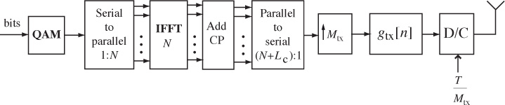
Figure 5.22 Block diagram of an OFDM transmitter. Often the upsampling and digital pulse shaping are omitted when rectangular pulse shapes are used. The inverse DFT is implemented using an inverse fast Fourier transform (IFFT).
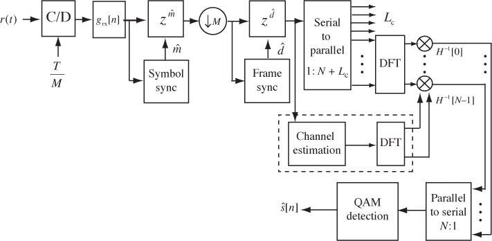
Figure 5.23 Block diagram of an OFDM receiver. Normally the matched filtering and symbol synchronization functions are omitted.
The key idea of OFDM, from the perspective of SC-FDE, is to insert the IDFT after the first serial-to-parallel converter in Figure 5.22. Given ![]() and a cyclic prefix of length Lc, the transmitter produces the sequence
and a cyclic prefix of length Lc, the transmitter produces the sequence

which is passed to the transmit pulse-shaping filter. The signal w[n] satisfies w[n] = w[n + N] for n = 0, 1, . . . , Lc − 1; therefore, it has a cyclic prefix. The samples {w[Lc], w[Lc + 1], . . . , w[N + Lc − 1]} correspond to the IDFT of ![]() . Unlike the SC-FDE case, the transmitted symbols can be considered to originate in the frequency domain. We do not use the frequency-domain notation for s[n] for consistency with the signal model.
. Unlike the SC-FDE case, the transmitted symbols can be considered to originate in the frequency domain. We do not use the frequency-domain notation for s[n] for consistency with the signal model.
We present the transmitter structure in Figure 5.22 to make the connection with SC-FDE clear. In OFDM, though, it is common to use rectangular pulse shaping where

This function is not bandlimited, so it cannot strictly speaking be implemented using the upsampling followed by digital pulse shaping as shown in Figure 5.22. Instead, it is common to simply use the “stair-step” response of the digital-to-analog converter to perform the pulse shaping. This results in a signal at the output of the DAC that takes the form
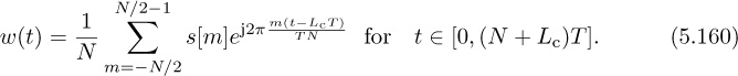
This interpretation shows how symbol s[m] rides on continuous-time carrier exp(j2πtm/NT) at baseband with a carrier of frequency 1/NT, which is also called the subcarrier bandwidth. This is one reason that OFDM is also called multicarrier modulation. We write the summation as shown in (5.160) to make it clear that frequencies around . . . , N − 3, N − 2, N − 1, 0, 1, 2, . . . are low frequencies whereas those around N/2 are high frequencies. Subcarrier n = 0 is known as the DC subcarrier, which is often assigned a zero symbol to avoid DC offset issues. The subcarriers near N/2 are often assigned zero symbols to facilitate spectral shaping.
Now we show how OFDM works. Consider the received signal as in (5.116). Discard the first Lc samples to form
Inserting (5.158) for w[n] and interchanging summations gives

Therefore, taking the DFT gives
for n = 0, 1, . . . , N − 1, and equalization simply involves multiplying by h−1[n]. Low SNR performance could be improved by multiplying by the LMMSE equalizer ![]() instead of by
instead of by h−1[n]. In terms of time-domain quantities,
The effective channel experienced by s[n] is h[n], which is a flat-fading channel. OFDM effectively converts a problem of equalizing a frequency-selective channel into that of equalizing a set of parallel flat-fading channels. Equalization thus simplifies a great deal versus time-domain linear equalization.
The terminology in OFDM systems is slightly different from that in single-carrier systems. Usually in OFDM, the collection of samples including the cyclic prefix ![]() is called an OFDM symbol. The constituent symbols
is called an OFDM symbol. The constituent symbols ![]() are called subsymbols. The OFDM symbol period is (N + Lc)T, and T is called the sample period. The guard interval, or cyclic prefix duration, is LcT. The subcarrier spacing is 1/(NT) and is the spacing between adjacent subcarriers as measured on a spectrum analyzer. The passband bandwidth is 1/T, assuming the use of a sinc pulse-shaping filter (which is not common; a rectangular pulse shape is used along with zeroing certain subcarriers).
are called subsymbols. The OFDM symbol period is (N + Lc)T, and T is called the sample period. The guard interval, or cyclic prefix duration, is LcT. The subcarrier spacing is 1/(NT) and is the spacing between adjacent subcarriers as measured on a spectrum analyzer. The passband bandwidth is 1/T, assuming the use of a sinc pulse-shaping filter (which is not common; a rectangular pulse shape is used along with zeroing certain subcarriers).
There are many trade-offs associated with selecting different parameters. Making N large while Lc is fixed reduces the fraction of overhead N/(N +Lc) due to the cyclic prefix. A larger N, though, means a longer block length and shorter subcarrier spacing, increasing the impact of time variation in the channel, Doppler, and residual carrier frequency offset. Complexity also increases with larger values as the complexity of processing per subcarrier grows with log2 N.
Consider an OFDM system where the OFDM symbol period is 3.2µs, the cyclic prefix has length Lc = 64, and the number of subcarriers is N = 256. Find the sample period, the passband bandwidth (assuming that a sinc pulse-shaping filter is used), the subcarrier spacing, and the guard interval.
Answer: The sample period T satisfies the relation T (256 + 64) = 3.2µs, so the sample period is T = 10ns. Then, the passband bandwidth is 1/T = 100MHz. Also, the subcarrier spacing is 1/(NT) = 390.625kHz. Finally, the guard interval is LcT = 640ns.
Noise impacts OFDM differently than SC-FDE. Now we examine what happens to the effective noise variance after equalization. In the presence of noise, and with perfect channel state information,
where v[n] = FN (υ[n]). Because linear combinations of Gaussian random variables are Gaussian, and the DFT is an orthogonal transformation, v[n] remains Gaussian with zero mean and variance ![]() . Therefore,
. Therefore, v[n]/h[n] is AWGN with zero mean and variance ![]() . Unlike SC-FDE, the noise enhancement varies with different subcarriers. When
. Unlike SC-FDE, the noise enhancement varies with different subcarriers. When h[n] is small for a particular value of n (close to a null in the spectrum), substantial noise enhancement is created. With SC-FDE there is also noise enhancement, but each detected symbol sees the same effective noise variance as in (5.156). With coding and interleaving, the error rate differences between SC-FDE and OFDM are marginal, unless other impairments like low-resolution DACs and ADCs or nonlinearities are included in the comparison (see, for example, [291, 102, 300, 192, 277]) when SC-FDE has a slight edge.
OFDM is in general more sensitive to RF impairments compared with SC-FDE and standard complex pulse-amplitude modulated signals. It is sensitive to nonlinearities because the ratio between the peak of the OFDM signal and its average value (called the peak-to-average power ratio) is higher in an OFDM system compared with a standard complex pulse-amplitude modulated signal. The reason is that the IDFT operation at the transmitter makes the signal more likely to have all peaks. Signal processing techniques can be used to mitigate some of the differences [166]. OFDM signals are also more sensitive to phase noise [264], gain and phase imbalance [254], and carrier frequency offset [75].
The OFDM waveform offers additional degrees of flexibility not found in SC-FDE. For example, the information rate can be adjusted to current channel conditions based on the frequency selectivity of the channel by changing the modulation and coding on different subcarriers. Spectral shaping is possible by zeroing certain symbols, as already described. Different users can even be allocated to subcarriers or groups of subcarriers in what is called orthogonal frequency-division multiple access (OFDMA). Many systems like IEEE 802.11a/g/n/ac use OFDM exclusively for transmission and reception. 3GPP LTE Advanced uses OFDM on the downlink and a variation of SC-FDE on the uplink where power backoff is more critical. IEEE 802.11ad supports SC-FDE as a mandatory mode and OFDM in a higher-rate optional mode. Despite their differences, both OFDM and SC-FDE maintain an important advantage of time-domain linear equalization: the equalizer complexity does not scale with L, as long as the cyclic prefix is long enough. Going forward, OFDM and SC-FDE are likely to continue to see wide commercial deployment.
5.3 Estimating Frequency-Selective Channels
When developing algorithms for equalization, we assumed that the channel state information ![]() was known perfectly at the receiver. This is commonly known as genie-aided channel state information and is useful for developing analysis of systems. In practice, the receiver needs to estimate the channel coefficients as engineering an all-knowing genie has proved impossible. In this section, we describe one method for estimating the channel in the time domain, and another for estimating the channel in the frequency domain. We also describe an approach for direct channel equalization in the time domain, where the coefficients of the equalizer are estimated from the training data instead of first estimating the channel and then computing the inverse. All the proposed methods make use of least squares.
was known perfectly at the receiver. This is commonly known as genie-aided channel state information and is useful for developing analysis of systems. In practice, the receiver needs to estimate the channel coefficients as engineering an all-knowing genie has proved impossible. In this section, we describe one method for estimating the channel in the time domain, and another for estimating the channel in the frequency domain. We also describe an approach for direct channel equalization in the time domain, where the coefficients of the equalizer are estimated from the training data instead of first estimating the channel and then computing the inverse. All the proposed methods make use of least squares.
5.3.1 Least Squares Channel Estimation in the Time Domain
In this section, we formulate the channel estimation problem in the time domain, making use of a known training sequence. The idea is to write a linear system of equations where the channel convolves only the known training data. From this set of equations, the least squares solution follows directly.
Suppose as in the frame synchronization case that ![]() is a known training sequence and that s[n] = t[n] for n = 0, 1, . . . , Ntr − 1. Consider the received signal in (5.87). We have to write y[n] only in terms of t[n]. The first few samples depend on symbols sent prior to the training data. For example,
is a known training sequence and that s[n] = t[n] for n = 0, 1, . . . , Ntr − 1. Consider the received signal in (5.87). We have to write y[n] only in terms of t[n]. The first few samples depend on symbols sent prior to the training data. For example,
Since prior symbols are unknown (they could belong to a previous packet or a message sent to another user, or they could even be zero, for example), they should not be included in the formulation. Taking n ∈ [L, Ntr − 1], though, gives

which is only a function of the unknown training data. We use these samples to form our channel estimator.
Collecting all the known samples together,

which is simply written in matrix form as
As a result, this problem takes the form of a linear parameter estimation problem, as reviewed in Section 3.5.
The least squares channel estimate, which is also the maximum likelihood estimate since the noise is AWGN, is given by
assuming that the Toeplitz training matrix T is invertible. Notice that the product (T*T)−1T can be computed offline ahead of time, so the actual complexity is simply a matrix multiplication.
To be invertible, the training matrix must be square or tall, which requires that
Generally, choosing Ntr much larger than L + 1 (the length of the channel) gives better performance. The full-rank condition can be guaranteed by ensuring that the training sequence is persistently exciting. Basically this means that it looks random enough. A typical design objective is to find a sequence such that T*T is (nearly) a scaled identity matrix I. This ensures that the noise remains nearly IID among other properties. Random training sequences with sufficient length usually perform well whereas t[n] = 1 will fail. Training sequences with good correlation properties generally satisfy this requirement, because the entries of T*T are different (partial) correlations of t[n].
Special training sequences can be selected from those known to have good correlation properties. One such design uses a cyclically prefixed training sequence. Let ![]() be a sequence with good periodic correlation properties. This means that the periodic correlation
be a sequence with good periodic correlation properties. This means that the periodic correlation ![]() satisfies the property that |Rp[k]| is small or zero for k > 0. Construct the training sequence
satisfies the property that |Rp[k]| is small or zero for k > 0. Construct the training sequence ![]() by prefixing
by prefixing ![]() with
with ![]() , which gives an Ntr = Np + L training sequence. With this construction
, which gives an Ntr = Np + L training sequence. With this construction
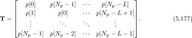
Then [T*T]k,ℓ = Rp[k − ℓ] contains lags of the periodic correlation function. Therefore, sequences with good periodic autocorrelation properties should work well when cyclically prefixed.
In the following examples, we present designs of T based on sequences with perfect periodic autocorrelation. This results in T*T = NpI and a simplified least squares estimate of ![]() . We consider the Zadoff-Chu sequences [70, 117] in Example 5.14 and Frank sequences [118] in Example 5.15. These designs can be further generalized to families of sequences with good cross-correlations as well; see, for example, the Popovic sequences in [267].
. We consider the Zadoff-Chu sequences [70, 117] in Example 5.14 and Frank sequences [118] in Example 5.15. These designs can be further generalized to families of sequences with good cross-correlations as well; see, for example, the Popovic sequences in [267].
Zadoff-Chu sequences are length Np sequences with perfect periodic autocorrelation [70, 117], which means that Rp[k] = 0 for k ≠ 0. They have the form
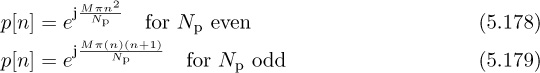
where M is an integer that is relatively coprime with Np, which could be as small as 1. Chu sequences are drawn from the Np-PSK constellation and have length Np.
Find a Chu sequence of length Np = 16.
Answer: We need to find an M that is coprime with Np. Since 16 has divisors of 2, 4, and 8, we can select any other number. For example, choosing M = 3 gives
which gives the sequence
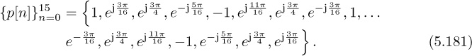
With this choice of training, it follows that T*T = NpI.
The Frank sequence [118] gives another construction of sequences with perfect periodic correlation, which uses a smaller alphabet compared to the Zadoff-Chu sequences. For n = mq + k,
where r must be coprime with q, q is any positive integer, and n ∈ [0, q2 − 1]. The length of the Frank sequence is then Np = q2 and comes from a q-PSK alphabet.
Find a length 16 Frank sequence.
Answer: Since the length of the Frank sequence is Np = q2, we must take q = 4. The only viable choice of r is 3. With this choice
for m ∈ [0, 3] and k ∈ [0, 3]. This gives the sequence
The Frank sequence also satisfies T but does so with a smaller constellation size, in this case 4-PSK. Note that a 4-QAM signal can be obtained by rotating each entry by exp(jπ/4).
A variation of the cyclic prefixed training sequence design uses both a prefix and a postfix. This approach was adopted in the GSM cellular standard. In this case, a sequence with good periodic correlation properties ![]() is prefixed by L samples
is prefixed by L samples ![]() and postfixed by the samples
and postfixed by the samples ![]() . This results in a sequence with length Ntr + 2L. The motivation for this design is that
. This results in a sequence with length Ntr + 2L. The motivation for this design is that

With perfect periodic correlation, the cross-correlation between p[n] and t[n] then has the form of
which looks like a discrete-time delta function plus some additional cross-correlation terms (represented by u; these are the values of Rpt[k] for k ≥ L). As a result, correlation with p[n], equivalently convolving with p*[(Np − n + 1)], directly produces an estimate of the channel for certain correlation lags. For example, assuming that s[n] = t[n] for n = 0, 1, . . . , Ntr − 1,
for n = Np, Np + 1, . . . , Np + L. In this way, it is possible to produce an estimate of the channel just by correlating with the sequence {p[n]} that is used to compose the training sequence {t[n]}. This has the additional advantage of also helping with frame synchronization, especially when the prefix size is chosen to be larger than L, and there are some extra zero values output from the correlation.
Another training design is based on Golay complementary sequences [129]. This approach is used in IEEE 802.ad [162]. Let ![]() and
and ![]() be length Ng Golay complementary sequences. Such sequences satisfy a special periodic correlation property
be length Ng Golay complementary sequences. Such sequences satisfy a special periodic correlation property

Furthermore, they also satisfy the aperiodic correlation property
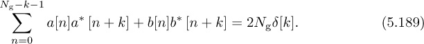
It turns out that the family of Golay complementary sequences is much more flexible than sequences with perfect periodic correlation like the Frank and Zadoff-Chu sequences. In particular, it is possible to construct such pairs of sequences from BPSK constellations without going to higher-order constellations. Furthermore, such sequence pairs exist for many choices of lengths, including for any Ng as a power of 2. There are generalizations to higher-order constellations. Overall, the Golay complementary approach allows a flexible sequence design with some additional complexity advantages.
Now construct a training sequence by taking ![]() , with a cyclic prefix and postfix each of length L, and naturally Ng > L. Then append another sequence constructed from
, with a cyclic prefix and postfix each of length L, and naturally Ng > L. Then append another sequence constructed from ![]() with a cyclic prefix and postfix as well. This gives a length Ntr = 2Ng + 4L training sequence. Assuming that s[n] = t[n] for n = 0, 1, . . . , Ntr − 1,
with a cyclic prefix and postfix as well. This gives a length Ntr = 2Ng + 4L training sequence. Assuming that s[n] = t[n] for n = 0, 1, . . . , Ntr − 1,
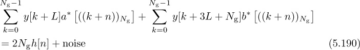
for n = 0, 1, . . . , Ng − 1. As a result, channel estimation can be performed directly by correlating the received data with the complementary Golay pair and adding the results. In IEEE 802.11ad, the Golay complementary sequences are repeated several times, to allow averaging over multiple periods, while also facilitating frame synchronization. They can also be used for rapid packet identification; for example, SC-FDE and OFDM packets use different sign patterns on the complementary Golay sequences, as discussed in [268].
An example construction of binary Golay complementary sequences is provided in Example 5.16. We provide an algorithm for constructing sequences and then use it to construct an example pair of sequences and a corresponding training sequence.
There are several constructions of Golay complementary sequences [129]. Let am[n] and bm[n] denote a Golay complementary pair of length 2m. Then binary Golay sequences can be constructed recursively using the following algorithm:
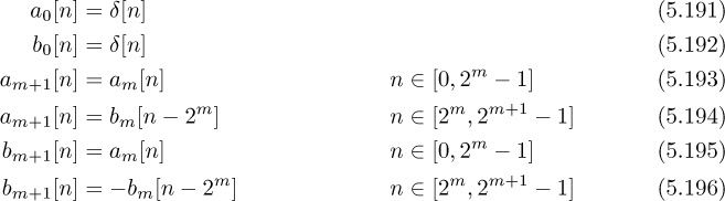
Find a length Ng = 8 Golay complementary sequence, and use it to construct a training sequence assuming L = 2.
Answer: Applying the recursive algorithm gives
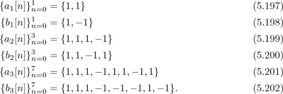
The resulting training sequence, composed of Golay complementary sequences with length L = 2 cyclic prefix and postfix, is
IEEE 802.15.3c 60GHz is a standard for high-data-rate WPAN. In this example, we review the preamble for what is called the high-rate mode of the SC-PHY. Each preamble has a slightly different structure to make them easy to distinguish. The frame structure including the preamble is shown in Figure 5.24. Let a128 and b128 denote vectors that contain length 128 complementary Golay sequences (in terms of BPSK symbols), and a256 and b256 vectors that contain length 256 complementary Golay sequences. From the construction in Example 5.16, a256 = [a128; b128] and b256 = [a128; −b128] where we use ; to denote vertical stacking as in MATLAB. The specific Golay sequences used in IEEE 802.15.3c are found in [159]. The preamble consists of three components:
1. The frame detection (SYNC) field, which contains 14 repetitions of a128 and is used for frame detection
2. The start frame delimiter (SFD), which contains [a128; a128; −a128; a128] and is used for frame and symbol synchronization
3. The channel estimation sequence (CES), which contains [b128; b256; a256; b256; a256] and is used for channel estimation
• Why does the CES start with b128?
Answer: Since a256 = [a128; b128], b128 acts as a cyclic prefix.
• What is the maximum channel order supported?
Answer: Given that b128 is a cyclic prefix, then Lc = 128 is the maximum channel order.
• Give a simple channel estimator based on the CES (assuming that frame synchronization and frequency offset correction have already been performed).
Answer: Based on (5.190),
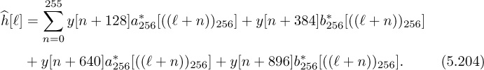
for ℓ = 0, 1, . . . , Lc.
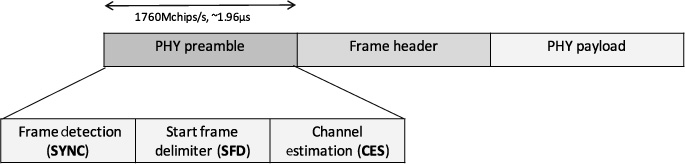
In this section, we presented least squares channel estimation based on a training sequence. We also presented several training sequence designs and showed how they can be used to simplify the estimation. This estimator was constructed assuming that the training data contains symbols. This approach is valid for standard pulse-amplitude modulated systems and SC-FDE systems. Next, we present several approaches for channel estimation that are specifically designed for OFDM modulation.
5.3.2 Least Squares Channel Estimation in the Frequency Domain
Channel estimation is required for frequency-domain equalization in OFDM systems. In this section, we describe several approaches for channel estimation in OFDM, based on either the time-domain samples or the frequency-domain symbols.
First, we describe the time-domain approach. We suppose that Ntr = N, so the training occupies exactly one complete OFDM symbol. It is straightforward to generalize to multiple OFDM symbols. Suppose that the training ![]() is input to the IDFT, and a length Lc cyclic prefix is appended, to create
is input to the IDFT, and a length Lc cyclic prefix is appended, to create ![]() . In the time-domain approach, the IDFT output samples
. In the time-domain approach, the IDFT output samples ![]() are used to estimate the time-domain channel coefficients, by building T in (5.173) from w[n] and then estimating the channel from (5.175). The frequency-domain channel coefficients are then obtained from
are used to estimate the time-domain channel coefficients, by building T in (5.173) from w[n] and then estimating the channel from (5.175). The frequency-domain channel coefficients are then obtained from ![]() . The main disadvantage of this approach is that the nice properties of the training sequence are typically lost in the IDFT transformation.
. The main disadvantage of this approach is that the nice properties of the training sequence are typically lost in the IDFT transformation.
Now we describe an approach where training is interleaved with unknown data in what are called pilots. Essentially the presence of pilots means that a subset of the symbols on a given OFDM symbol are known. With enough pilots, we show that it is possible to solve a least squares channel estimation problem using only the data that appears after the IDFT operation [338].
Suppose that training data is sent on a subset of all the carriers in an OFDM symbol; using all the symbols is a special case. Let P = {p1, p2, . . . , pP } denote the indices of the subcarriers that contain known training data. The approach we take is to write the observations as a function of the unknown channel coefficients. First observe that by writing the frequency-domain channel in terms of the time-domain coefficients,
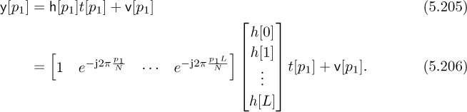
Collecting the data from the different pilots together:

This can now be written compactly as
The matrix P has the training pilots on its diagonal. It is invertible for any choice of nonzero pilot symbols. The matrix E is constructed from samples of DFT vectors. It is tall and full rank as long as the number of pilots P ≥ L + 1. Therefore, with enough pilots, we can compute the least squares solution as
This approach allows least squares channel estimation to be applied based only on training at known pilot locations. The choice of pilot sequences with pilot estimation is not as important as in the time-domain approach; the selection of pilot locations is more important as this influences the rank properties of E. The approach can be extended to multiple OFDM symbols, possibly at different locations for improved performance.
An alternative approach for channel estimation in the frequency domain is to interpolate the frequency-domain channel estimates instead of solving a least squares problem [154]. This approach makes sense when training is sent on the same subcarrier across OFDM symbols, to allow some additional averaging over time.
Consider a comb-type pilot arrangement where P pilots are evenly spaced and Nc = N/P. This uniform spacing is optimum under certain assumptions for LMMSE channel estimation in OFDM systems [240] and for least squares estimators if P*P is a scaled identity matrix. Let ![]() be the channel estimated at the pilot locations for c = 0, 1, . . . , P −1 with
be the channel estimated at the pilot locations for c = 0, 1, . . . , P −1 with ![]() and
and ![]() to account for wrapping effects. This estimate is obtained by averaging over multiple observations of
to account for wrapping effects. This estimate is obtained by averaging over multiple observations of y[pk] in multiple OFDM symbols. Using second-order interpolation, the missing channel coefficients are estimated as [77]
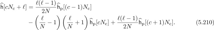
In this way, the frequency-domain channel coefficients may be estimated directly from the pilots without solving a higher-dimensional least squares problem. With a similar total number of pilots, the performance of the time-domain and interpolation algorithms can be similar [154].
There are other approaches for channel estimation that may further improve performance. For example, if some assumptions are made about the second-order statistics of the channel, and these statistics are known at the receiver, then LMMSE methods may be used. Several decibels of performance improvement, in terms of uncoded symbol error rate, may be obtained through MMSE [338]. Pilots may also be distributed over multiple OFDM symbols, on different subcarriers in different OFDM symbols. This allows two-dimensional interpolation, which is valuable in channels that change over time [196]. The 3GPP LTE cellular standard includes pilots distributed across subcarriers and across time.
In this example, we explore the preamble structure used in IEEE 802.11a, shown in Figure 5.25, and explain how it is used for channel estimation [160, Chapter 17]. A similar structure is used in IEEE 802.11g, with some backward compatibility support for 802.11b, and in IEEE 802.11n, with some additions to facilitate multiple-antenna transmission. The preamble in IEEE 802.11a consists of a short training field (STF) and a channel estimation field (CEF). Each field has the duration of two OFDM symbols (8µs) but is specially constructed. In this problem, we focus on channel estimation based on the CEF, assuming that frame synchronization and carrier frequency offset correction have been performed.
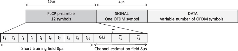
Figure 5.25 Frame structure defined in the IEEE 802.11a standard. In the time domain, the waveforms t1 through t10 are identical (ten repetitions of short training) and T1 and T2 are the same (two repetitions of long training). The Physical Layer Convergence Procedure (PLCP) is used to denote the extra training symbols inserted to aid synchronization and training.
The CEF of IEEE 802.11a consists of two repeated OFDM symbols, each containing training data, preceded by an extra-long cyclic prefix. Consider a training sequence of length N = 64 with values
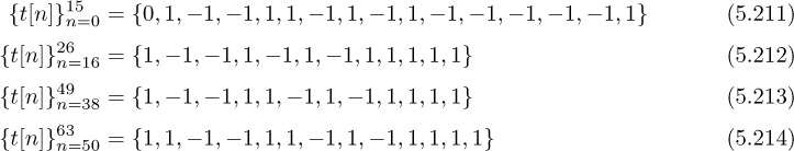
where all other subcarriers are zero. IEEE 802.11a uses zero subcarriers to help with spectral shaping; a maximum of only 52 subcarriers is used. The n = 0 subcarrier corresponds to DC and is also zero. The CEF is constructed as
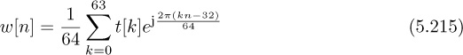
for n = 0, 1, . . . , 159. Essentially the CEF has one extended cyclic prefix of length Lc = 32 (extended because it is longer than the normal Lc = 16 prefix used in IEEE 802.11a) followed by the repetition of two IDFTs of the training data. The repetition is also useful for frequency offset estimation and frame synchronization described in Section 5.4.4. Time-domain channel estimation can proceed directly using (5.215). For estimation from the frequency domain, we define two slightly different truncated received signals ![]() and
and ![]() for n = 0, 1, . . . , 63. Taking the DFT gives
for n = 0, 1, . . . , 63. Taking the DFT gives ![]() and
and ![]() . The parts of the received signal corresponding to the nonzero training
. The parts of the received signal corresponding to the nonzero training ![]() ,
, ![]() ,
, ![]() , and
, and ![]() can then be used for channel estimation by using a linear equation of the form
can then be used for channel estimation by using a linear equation of the form
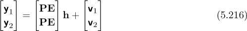
and finding the least squares solution.
5.3.3 Direct Least Squares Equalizer
In the previous sections, we developed channel estimators based on training data. These channel estimates can be used to devise equalizer coefficients. At each step in the process, both channel estimation and equalizer computation create a source of error since they involve solving least squares problems. As an alternative, we briefly review an approach where the equalizer coefficients are estimated directly from the training data. This approach avoids the errors that occur in two steps, giving somewhat more noise robustness, and does not require explicit channel estimation.
To formulate this problem, again consider the received signal in (5.87), and the signal after equalization in (5.96), which gives an expression for ![]() . We now formulate a least squares problem based on the presence of the known training data s[n] = t[n] for n = 0, 1, . . . , Ntr. Given the location of this data, and suitably time shifting the observed sequence, gives
. We now formulate a least squares problem based on the presence of the known training data s[n] = t[n] for n = 0, 1, . . . , Ntr. Given the location of this data, and suitably time shifting the observed sequence, gives

for n = 0, 1, . . . , Ntr. Building a linear equation:

In matrix form, the objective is to solve the following linear system for the unknown equalizer coefficients:
If Lf + 1 > Ntr, then Ynd is a fat matrix, and the system of equations is undetermined. This means that there is an infinite number of exact solutions. This, however, tends to lead to overfitting, where the equalizer is perfectly matched to the observations in Ynd. A more robust approach is to take Lf ≤ Ntr − 1, turning Ynd into a tall matrix. It is reasonable to assume that Yndx is full rank because of the presence of additive noise in y[n]. Under this assumption, the least squares solution is
The squared error is measured as ![]() . The squared error can be minimized further by choosing nd such that Jf[nd] is minimized.
. The squared error can be minimized further by choosing nd such that Jf[nd] is minimized.
A block diagram including direct equalization is illustrated in Figure 5.26. The block diagram assumes that the equalization computation block optimizes over the delay and outputs the corresponding filter and required delay. Direct equalization avoids the separate channel estimation and equalizer computation blocks.
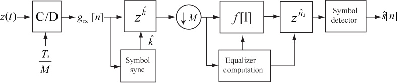
Figure 5.26 A complex pulse-amplitude modulation receiver with direct equalizer estimation and linear equalization
The direct and indirect equalization techniques have different design trade-offs. With the direct approach, the length of the training determines the maximum length of the equalizer. This is a major difference between the direct and indirect methods. With the indirect method, an equalizer of any order Lf can be designed. The direct method, however, avoids the error propagation where the estimated channel is used to compute the estimated equalizer. Note that with a small amount of training the indirect method may perform better since a larger Lf can be chosen, whereas a direct method may be more efficient when Ntr is larger. The direct method also has some robustness as it will work even when there is model mismatch, that is, when the LTI model is not quite valid or there is interference. Direct equalization can be done perfectly in multichannel systems as discussed further in Chapter 6.
5.4 Carrier Frequency Offset Correction in Frequency-Selective Channels
In this section, we describe the carrier frequency offset impairment for frequency-selective channels. We present a discrete-time received signal model that includes frequency offset. Then we examine several carrier frequency offset estimation algorithms. We also remark how each facilitates frame synchronization.
5.4.1 Model for Frequency Offset in Frequency-Selective Channels
In Section 5.1.6, we introduced the carrier frequency offset problem. In brief, carrier frequency offset occurs when the carrier used for upconversion and the carrier used for downconversion are different. Even a small difference can create a significant distortion in the received signal.
We have all the ingredients to develop a signal model for frequency offset in frequency-selective channels. Our starting point is to recall (5.67), which essentially says that carrier frequency offset multiplies the matched filtered received signal by ej2πfet. Sampling at the symbol rate, and using our FIR model for the received signal in (5.87), we obtain

It is possible to further generalize (5.221) to include frame synchronization by including a delay of d. Correction of carrier frequency offset therefore amounts to estimating ![]() and then derotating the received signals e−j2π
and then derotating the received signals e−j2π![]() ny[n].
ny[n].
In the frequency-flat case, the frequency offset creates a successive rotation of each symbol by exp(j2π![]() n). In the frequency-selective case, this rotation is applied to the convolutive mixture between the symbols and the channel. As a result, the carrier frequency offset distorts the data that would otherwise be used for channel estimation and equalization. Even if training data is available, it does not lead directly to a simple estimator. A direct extension of what we have studied leads to a joint carrier frequency offset and channel estimation problem, which has high complexity. In this section, we review several lower-complexity methods for frequency offset estimation, which rely on special signal structure to implement.
n). In the frequency-selective case, this rotation is applied to the convolutive mixture between the symbols and the channel. As a result, the carrier frequency offset distorts the data that would otherwise be used for channel estimation and equalization. Even if training data is available, it does not lead directly to a simple estimator. A direct extension of what we have studied leads to a joint carrier frequency offset and channel estimation problem, which has high complexity. In this section, we review several lower-complexity methods for frequency offset estimation, which rely on special signal structure to implement.
5.4.2 Revisiting Single-Frequency Estimation
For our first estimator, we revisit the estimator proposed in Example 5.8 and show how it can also be used in frequency-selective channels with minimal changes. This type of sinusoidal training was used in the GSM system through a special input to the GMSK (Gaussian minimum shift keying) modulator.
Let us choose as a training sequence t[n] = exp(j2πftn) for n = 0, 1, . . . , Ntr − 1 where ft is a discrete-time design frequency. Consider the received signal (5.87) with s[n] = t[n] for n = 0, 1, . . . , Ntr − 1. Discarding samples that do not depend on the training, we have the received signal
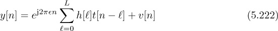
for n = L, L + 1, . . . , Ntr − 1. Substituting for the training signal,

where h (ej2πft) is the DTFT of h[n]. Derotating by the known frequency of the training signal,
This has the form of (5.72) from Example 5.8. As a result, the estimators for frequency-flat frequency offset estimation using sinusoidal training can also be applied to the frequency-selective case.
The main signal processing trick in deriving this estimator was to recognize that signals of the form exp(j2πftn) are eigenfunctions of discrete-time LTI systems. Because the unknown channel is FIR with order L, and the training Ntr > L, we can discard some samples to remove the edge effects. The frequency ft could be selected of the form k/Ntr to take advantage, for example, of subsequent frequency-domain processing in the modem.
The main advantage of single-frequency estimation is that any number of good algorithms can be used for estimation; see, for example, [330, 3, 109, 174, 212, 218] among others. The disadvantage of this approach is that performance is limited by h (ej2πft). Since the channel is frequency selective by assumption and has L zeros because it is FIR of order L, it could happen that the chosen frequency of ft is close to a zero of the channel. Then the SNR for the estimator would be poor. The sinusoidal training also does not lead to a sharp correlation peak that can be used for frame detection. Furthermore, if used to construct T in (5.175), it would in fact not have full rank, and thus it could not be used for channel estimation. As a result, we now review other approaches for carrier frequency offset estimation.
5.4.3 Frequency Offset Estimation and Frame Synchronization Using Periodic Training for Single-Carrier Systems
There are several different algorithms for frequency offset estimation using different properties of the transmitted signal such as periodicity, constant modulus, and so on. One of the most elegant methods was proposed by Moose [231] and has since been studied extensively. This method relies on a special periodic training sequence that permits joint carrier frequency offset estimation and frame synchronization. The training sequences can also be used for channel estimation. Periodic training has found application in IEEE 802.11a/g/n/ac systems and others. In this section, we consider the application of periodic training to a single-carrier system, though note that Moose’s original application was to OFDM. We deal with the case of OFDM, including another algorithm called the Schmidl-Cox approach [296], in the next section.
Now we explain the key idea behind the Moose algorithm from the perspective of using just two repeated training sequences. Other extensions are possible with multiple repetitions. Consider the framing structure illustrated in Figure 5.27. In this frame, a pair of training sequences are sent together, followed by a data sequence.

Figure 5.27 The framing used in the Moose estimator. A pair of training sequences are followed by data.
The Moose algorithm exploits the periodicity in the training sequence. Let the training sequence start at n = 0. Then
for n = 0, 1, . . . , Ntr − 1. Note that symbols s[n] for n < 0 and n ≥ 2Ntr are unknown (they are either zero or correspond to the unknown portions of the data).
Now we explain the trick associated with periodicity in the training data. For n ∈ [L, Ntr − 1],

Using the fact that s[n + Ntr] = s[n] = t[n] for n = 0, 1, . . . , Ntr − 1:
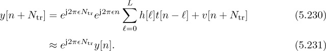
To see the significance of this result, remember that the channel coefficients ![]() are unknown! The beauty of (5.231) is that it is a function of known observations and only the unknown frequency offset. Essentially, the periodicity establishes a relationship between different parts of the received signal y[n]. This is an amazing observation, since it does not require any assumptions about the channel.
are unknown! The beauty of (5.231) is that it is a function of known observations and only the unknown frequency offset. Essentially, the periodicity establishes a relationship between different parts of the received signal y[n]. This is an amazing observation, since it does not require any assumptions about the channel.
There are several possible approaches for solving (5.231). Note that this is slightly different from the single-frequency estimator because of the presence of y[n] on the right-hand side of (5.231). The direct least squares approach is not possible since the unknown parameter is present in the exponent of the exponential. A solution is to consider a relaxed problem
solving for ![]() and then finding
and then finding ![]() from the phase. This problem is similar to flat-fading channel estimation in Section 5.1.4. Using (5.47), we can write
from the phase. This problem is similar to flat-fading channel estimation in Section 5.1.4. Using (5.47), we can write
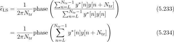
where we can neglect the denominator since it does not contribute to the phase estimate. Despite the relaxation in this derivation, it turns out that this is also the maximum likelihood estimator [231].
There is an important limitation in the Moose algorithm. Because of the periodicity of discrete-time exponentials, the estimate of ![]() is accurate only for
is accurate only for ![]() or equivalently
or equivalently
which in terms of the actual frequency offset means
This reveals an interesting trade-off in the estimator performance. Choosing larger Ntr improves the estimate since there is more noise averaging, but it reduces the range of offsets that can be corrected. A way of solving this problem is to use multiple repetitions of a short training sequence. IEEE 802.11a and related standards use a combination of both repeated short training sequences and long training sequences.
Compute the maximum allowable offset for a 1Ms/s-QAM signal, with fc = 2GHz and Nt = 10.
Answer:
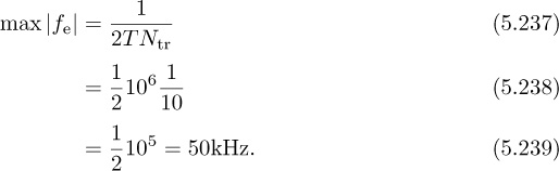
In terms of parts per million, we need an oscillator that can generate a 2GHz carrier with an accuracy of 50e3/2e9 = 25ppm.
Consider a wireless system where each data frame is preceded by two training blocks, each consisting of Ntr = 12 training symbols. Let the symbol period be T = 4µs. What is the maximum frequency offset that can be corrected using training?
Answer: The maximum frequency offset that can be corrected using training is ![]() = 1/(2Ntr) ≈ 0.0417 or fe = 1/(2TNtr) ≈ 10.417kHz.
= 1/(2Ntr) ≈ 0.0417 or fe = 1/(2TNtr) ≈ 10.417kHz.
The Moose algorithm also provides a nice way of performing frame synchronization. The observation is that the correlation peak should occur when the pair of training sequences is encountered at the receiver. Essentially, this involves solving for the offset d such that

where the search is performed over a reasonable set of possible values of d. For example, the analog RF may perform carrier sensing, activating the ADCs only when a sufficiently strong signal is present.
The denominator normalization in the frame synchronization is required to avoid false positives when there is no signal present. An alternative solution, which is somewhat more robust in this case, involves normalizing by both observed vectors as in
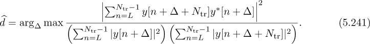
No matter which algorithm is used, both result in the same thing: a joint solution to the frame synchronization and frequency offset estimation and correction problem in an intersymbol interference channel.
Channel estimation is also facilitated using the Moose algorithm. Once the frequency offset is estimated and corrected, and the frame is synchronized, the pair of training sequences can be combined for channel estimation. As a result, periodic training provides a flexible approach for solving key receiver functions in frequency-selective channels.
An illustration of the complete receiver can be found in Figure 5.28. The frequency offset estimation and correction are performed prior to channel estimation and equalization but after the downsampling operation. Better performance could be achieved by operating before the downsampling, replacing the symbol synchronizer, but this is usually practical only for smaller values of Mrx.

Figure 5.28 A single-carrier receiver with frequency offset estimation and correction, frame synchronization, channel estimation, and linear equalization. The linear equalization could be replaced by an SC-FDE receiver structure with no other changes required.
We conclude this section with a detailed example that describes how to use the preamble structure in IEEE 802.15.3c single-carrier mode and in IEEE 802.11a.
Consider the IEEE 802.15.3c preamble structure as described in Example 5.17 for the high-rate mode of the SC-PHY. In this example, we describe how the SYNC field is used for carrier frequency offset estimation and frame synchronization. Note that the standard just describes the preamble itself; it does not describe how the receiver signal processing should be applied to the preamble. A good description of digital synchronization algorithms for IEEE 802.15.3c is found in [204].
The SYNC field can be used for frame synchronization and carrier frequency offset estimation. The SYNC field contains 14 repetitions of a128. Because the maximum supported channel length is Lc = 128, though, the first repetition acts as a cyclic prefix. Therefore, we can use the following frame detection algorithm:
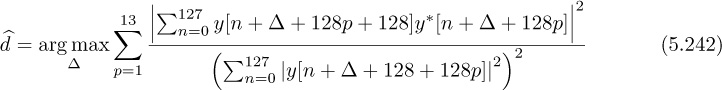
where we have put the packet energy in the denominator to make the algorithm more robust when averaging over multiple repetitions. The carrier frequency offset can then be estimated from either averaging the offset with each period and combining or taking the phase of the average as

The maximum absolute offset correctable is 1/256.
In packet-based wireless systems, the digital part of the receiver may be in sleep mode to save power. As a result, the analog may make an initial determination that there is a signal of interest, for example, if the signal exceeds a threshold. The SYNC field can be used for this initial determination. In the process, though, some samples may be lost, and not all repetitions will be available for averaging. As a result, it may make sense to average over fewer repetitions in (5.242). It also may make sense to either defer frequency offset correction or make a correction based on this tentative estimate (called a coarse correction), then proceed with further correction and refinement using the SFD field.
Consider the IEEE 802.11a preamble structure as described in Example 5.18. In this example, we explain the coarse frequency offset using the STF field and the fine frequency offset using the CEF field. We assume B = 20MHz bandwidth. The STF field (in the time domain) consists of ten repetitions (created by zeroing subcarriers as described in Section 5.4.4). The CEF field has two repetitions. Sampled at T = 1/B, each repetition of the STF contains 16 samples, whereas the CEF has two repetitions of 64 samples with a length 32 cyclic prefix.
The STF field is used for functions such as packet detection, automatic gain control (AGC), and coarse synchronization. Because the RF may be powering up, and the AGC adjusting, not all of the ten repetitions are typically used for synchronization. For example, suppose that three repetitions are used with the first acting as a cyclic prefix. Then we use the following frame detection algorithm:
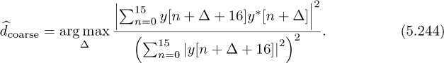
The coarse carrier frequency offset estimate is then

The maximum absolute frequency offset correctable is 1/32.
Next, we correct for the coarse frequency offset to create the new signal ![]() . Using this corrected signal, we then search for the long training sequence:
. Using this corrected signal, we then search for the long training sequence:
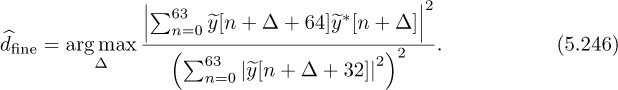
The coarse frame synchronization estimate can be used to reduce the search space of possible offsets. The fine carrier frequency offset estimate is then

The two-step approach allows an initial frequency offset estimate with a larger correction range, but it is noisier in the first step because of the use of only 16 samples. Then, in the second step, it is possible to get a more accurate estimate by using 64 samples with a smaller range, assuming the first phase corrected for the larger errors.
5.4.4 Frequency Offset Estimation and Frame Synchronization Using Periodic Training for OFDM Systems
OFDM is sensitive to carrier frequency offset. The reason is essentially that carrier frequency offset over the duration of an OFDM symbol creates problems because the DFT is taken over the whole OFDM symbol period. Small variations are compounded by the DFT operation into bigger variations.
Frequency offset correction algorithms for OFDM systems are similar to their time-domain counterparts. The method in Section 5.4.2 can be applied to OFDM by sending a OFDM symbol with just a single subcarrier active. The method in Section 5.4.3 can be applied directly only to multiple repetitions of OFDM systems. In this section, we develop another carrier frequency offset estimator that works on the periodicity created in one OFDM symbol. It also has an advantage over the Moose method in that it allows a larger range of offsets to be corrected, when used with a second specially designed OFDM symbol.
We start by explaining how to create periodicity in a single OFDM symbol. The key insight is to make a portion of the transmitted signal look periodic and then to apply the same technique as before. Suppose that we construct an OFDM symbol where all the odd subcarriers are zero. Then
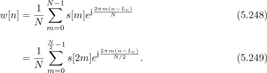
This looks like an extended discrete-time sinusoid with carrier 2π(N/2). As a result, for n ∈ [Lc, Lc + N/2],
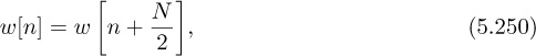
which means that the OFDM signal contains a portion that is periodic. As a result, the Moose algorithm can be applied directly to this setting.
Consider the case where frame synchronization has already been performed. The received signal model is

Discarding the cyclic prefix,
Because of the periodicity,
Then the Moose frequency offset estimator is
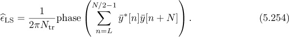
As before, it is possible to perform OFDM symbol synchronization (or frame synchronization) and frequency offset estimation jointly using this correlation method. The OFDM training symbol can even be used for channel estimation as this is just a special case of the comb-type pilot arrangement described in Section 5.3.2.
The maximum correctable carrier frequency offset is

As a result, the Moose algorithm can essentially correct for continuous-time offsets that are less than one subcarrier spacing 1/(NT). In an OFDM system, N may be quite large. This would in turn reduce the range of correctable offsets. Thus, it is of interest to develop techniques to enhance the range. One such approach is the Schmidl-Cox algorithm [296].
Consider an OFDM system with two training OFDM symbols. In the first symbol, all the odd subcarriers are zero. The even subcarriers ![]() are 4-QAM training symbols, which are nominally just a pseudo-noise sequence. The presence of zeros ensures that there is periodicity in the first OFDM symbol. Let
are 4-QAM training symbols, which are nominally just a pseudo-noise sequence. The presence of zeros ensures that there is periodicity in the first OFDM symbol. Let ![]() be a set of 4-QAM training symbols sent on the second OFDM symbol, without zeros. Further suppose that the even training symbols are selected such that
be a set of 4-QAM training symbols sent on the second OFDM symbol, without zeros. Further suppose that the even training symbols are selected such that ![]() where
where ![]() is another sequence with good periodic correlation properties. Effectively, the training data on even subcarriers of the second OFDM symbol is differentially encoded.
is another sequence with good periodic correlation properties. Effectively, the training data on even subcarriers of the second OFDM symbol is differentially encoded.
The Schmidl-Cox algorithm works as follows. Let the frequency offset be written as
where q is called the integer offset and ![]() frac is the fractional offset. Because
frac is the fractional offset. Because
the expression (5.253) is able to account for only fractional frequency offsets. Suppose that the estimator in (5.254) is used to estimate the fractional frequency offset. Further suppose that the estimate is perfect and is then removed by multiplying by exp(−j2π![]() fracN/2), leaving the received signal after correction as
fracN/2), leaving the received signal after correction as

Discarding the cyclic prefix and taking the DFT gives
for k = 0, 1, . . . , N − 1. The received signals corresponding to each training symbol use the index k = 0, 1, . . . , N − 1:

Now we exploit the fact that the training on the even subcarriers was differentially encoded. Consider

where ![]() contains the products with the noise terms. Because
contains the products with the noise terms. Because ![]() has good periodic correlation properties, a least-squares-type problem can be formulated and used to find the shift with a correlation peak:
has good periodic correlation properties, a least-squares-type problem can be formulated and used to find the shift with a correlation peak:
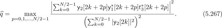
Based on this integer offset estimate, the received samples can be corrected by ![]() . Then the second OFDM training symbol can be used to estimate the channel (possibly combined with the first OFDM symbol as well).
. Then the second OFDM training symbol can be used to estimate the channel (possibly combined with the first OFDM symbol as well).
The final frequency offset estimate obtained with the Schmidl-Cox algorithm is
When both fractional and integer offset corrections are applied, a large range of offsets can be corrected. While it seems like very large offsets can be corrected, recall that the system model was derived assuming a small offset. A large offset would shift part of the desired signal outside the baseband lowpass filter, rendering the signal models inaccurate. In practice, this approach should be able to correct for offsets corresponding to several subcarriers, depending on the analog filtering, digital filtering, and extent over oversampling.
Like the Moose method, the Schmidl-Cox approach can also be used for OFDM symbol synchronization, by looking for a correlation peak around the first OFDM symbol as
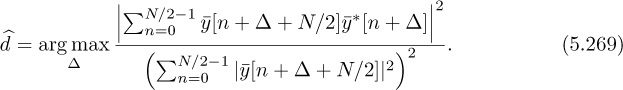
There is one distinct point of difference, though. With OFDM, there is also a cyclic prefix and often Lc > L. In this case, then
for n = L, L + 1, . . . , Lc, Lc + 1, . . . , N + Lc − 1. This means that there will be some ambiguity in (5.269), in that there may be several values of d that are close, especially when Lc is much larger than L. This creates a plateau in the symbol synchronization algorithm [296]. Any value within the plataeu, however, should give acceptable performance if the estimated channel has order Lc, but if the smaller channel length of L is assumed, then performance may suffer. Other training sequence designs can improve the sharpness of the frame synchronization, specifically with multiple repetitions along with a sign change among the different repetitions [306].
A system block diagram with OFDM and frame synchronization, channel estimation, and carrier frequency offset correction is illustrated in Figure 5.29. One frequency offset correction block is shown, but this could be broken up into two pieces corresponding to integer and fine offsets.
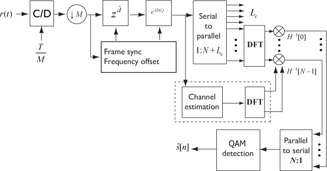
Figure 5.29 OFDM receiver frequency offset estimation and correction, channel estimation, and linear equalization. The matched filtering and symbol sampling are omitted as they are often not performed in OFDM.
In this example, we show how the STF in IEEE 802.11a is constructed to have periodicity. The STF is generated from a special training sequence with 12 nonzero values constructed as

for k = 0, 1, . . . , 15 and the other undefined values of the training are zero.
The presence of zeros in (5.271) is a result of the need for eliminating the DC subcarrier and spectral shaping, similar to the design of the CEF. Based on this training sequence,
for n = 0, 1, . . . , 159. The time-domain waveform thus contains ten repetitions of length 16.