Example of a Contour Plot
To create a contour plot, you need two variables for the x- and y-axes and at least one more variable for contours. You can also use several y-variables. This example uses the Little Pond.jmp sample data table. X and Y are coordinates of a pond. Z is the depth.
1. Open the Little Pond.jmp sample data table.
2. Select Graph > Contour Plot.
3. Select the X and Y coordinates and click X.
4. Select the depth, Z, and click Y.
Note: In a contour plot, the X1 and X2 roles are used for the X and Y axes.
5. Click Specify.
6. In the Contour Specification window, select # of Contours as 7.
7. Select Minimum as -4.
8. Select Maximum as 8.
9. Click OK.
Figure 6.2 Example of a Contour Plot with Legend
The x- and y-axes are coordinates and the contour lines are defined by the depth variable. This contour plot is essentially a map of a pond showing depth.
Launch the Contour Plot Platform
Launch the Contour Plot platform by selecting Graph > Contour Plot.
By default, the contour levels used in the plot are values computed from the data. You can specify your own number of levels and level increments in the Launch window before you create the plot. You can also do so in the red triangle menu for Contour Plot after you create the plot. You can use a column formula to compute the contour variable values.
Figure 6.3 The Contour Plot Launch Window
|
Y
|
Columns assigned to the Y role are used as variables to determine the contours of the plot. You must specify at least one, and you can specify more than one.
You can also assign a column with a formula to this role. If you do so, the formula should be a function of exactly two variables. Those variables should be the x variables entered in the Launch window.
|
|
X
|
Columns assigned to the X role are used as the variables for the x- and y-axes. You must specify exactly two columns for X.
|
|
By
|
This option produces a separate graph for each level of the By variable. If two By variables are assigned, a separate graph for each possible combination of the levels of both By variables is produced.
|
|
Options:
|
|
|
Contour Values
|
Specify your own number of levels and level increments.
|
|
Fill Areas
|
Fill the areas between contour lines using the contour line colors.
|
|
Use Table Data
Specify Grid
|
Most often, you construct a contour plot for a table of recorded response values. In that case, Use Table Data is selected and the Specify Grid button is unavailable.
However, if a column has a formula and you specify that column as the response (Y), the Specify Grid button becomes available. When you click Specify Grid, you can define the contour grid in any way, regardless of the rows in the existing data table. This feature is also available with table templates that have one or more columns defined by formulas but no rows.
|
For more information about the launch window, see Using JMP.
The Contour Plot
Follow the instructions in “Example of a Contour Plot” to produce the plot shown in Figure 6.4.
The legend for the plot shows individual markers and colors for the Y variable. Replace variables in the plot by dragging and dropping a variable, in one of two ways: swap existing variables by dragging and dropping a variable from one axis to the other axis; or, click on a variable in the Columns panel of the associated data table and drag it onto an axis.
For information about additional options for the report, see “Contour Plot Platform Options”.
Figure 6.4 The Contour Plot Report
Contour Plot Platform Options
Using the options in the red triangle menu next to Contour Plot, you can tailor the appearance of your contour plot and save information about its construction.
|
Show Data Points
|
Shows or hides (x, y) points. The points are hidden by default.
|
|
Show Missing Data Points
|
Shows or hides points with missing y values. Only available if Show Data Points is selected.
|
|
Show Contours
|
Shows or hides the contour lines or fills. The contour lines are shown by default.
|
|
Show Boundary
|
Shows or hides the boundary of the total contour area. The boundary is shown by default.
|
|
Show Control Panel
|
Shows or hides the Alpha slider that allows you to change the Alpha shapes filter.
Note: This option requires a saved triangulation data table. See “Contour Plot Save Options” for details.
|
|
Transform
|
If the contour plot includes a Color role, the Transform option is enabled. See “Example of Triangulation, Transform, and Alpha Shapes” for details.
None
The triangulation is computed without any scaling to coordinates using Delaunay triangulation. This is the default selection.
Range Normalized
The X1/X2 values are both be scaled to [0,1] prior to computing the triangulation. If the X1/X2 limits are different then this is a non-uniform scale. This can result in a different triangulation than the None option because the Delaunay triangles are dependent on the aspect ratio of the data. This option may be more desirable in cases where the X1/X2 units are very different. This was the default selection in JMP v10.
|
|
Fill Areas
|
Fills the areas between the contours with a solid color. It is the same option that is available in the Launch window. If you leave it deselected in the Launch window, you can see the line contours before filling the areas.
See “Fill Areas”.
|
|
Label Contours
|
Shows or hides the label (z-value) of the contour lines.
|
|
Color Theme
|
Select another color theme for the contours.
|
|
Reverse Colors
|
Reverses the order of the colors assigned to the contour levels.
|
|
Change Contours
|
Set your own number of levels and level increments.
|
|
Save
|
This menu has options to save information about contours, triangulation, and grid coordinates to data tables.
|
|
Script
|
This menu contains commands that are available to all platforms. They enable you to redo the analysis or save the JSL commands for the analysis to a window or a file. For more information, see Using JMP.
|
Fill Areas
If you select Fill Areas, the areas between contour lines are filled with the contour line colors. This option is available in the Launch window and in the red triangle menu for Contour Plot. Figure 6.5 shows a plot with contour lines on the left and a plot with the contour areas filled on the right.
Figure 6.5 Comparison of Contour Lines and Area Fills
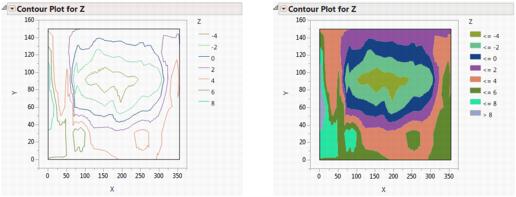
Areas are filled from low to high values. An additional color is added in the filled contour plot for the level above the last, and highest, contour line.
Contour Specification
If you do not select options in the Launch window, the default plot spaces the contour levels equally within the range of the Y variable. The default colors are assigned via the Continuous Color Theme in Preferences. You can see the colors palette with the Colors command in the Rows menu or by right-clicking on an item in the Contour Plot legend.
You can specify contour levels either in the Launch window (the Specify button) or in the report window from the red triangle menu for Contour Plot (the Specify Contours option).
Figure 6.6 Example of Contour Specification: Launch Window (on the left) and Menu (on the right)
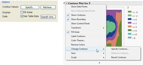
Specify
This option is both in the Launch window and on the red triangle menu for Contour Plot (the Specify Contours option).
Selecting this option displays the Contour Specification window. See Figure 6.7. Using this window, you can do the following:
• change the number of contours
• specify minimum and maximum values to define the range of the response to be used in the plot
• change the increment between contour values
You supply any three of the four values, and the remaining value is computed for you. Click on the check box to deselect one of the numbers and automatically select the remaining check box.
Figure 6.7 The Contour Specification Window
Colors are automatically assigned and are determined by the number of levels in the plot. After the plot appears, you can right-click (press CONTROL and click on the Macintosh) on any contour in the plot legend and choose from the JMP color palette to change that contour color.
Retrieve
This option is both in the Launch window (the Retrieve button) and on the red triangle menu for Contour Plot (the Retrieve Contours option).
Note: Neither the button nor the menu option are active unless there is an open data table in addition to the table that has the contour plotting values. When you click Retrieve or select Retrieve Contours, a window with a list of open data tables appears.
Using this option, you can retrieve the following from an open JMP data table:
• the number of contours
• an exact value for each level
• a color for each level
From the list of open data tables, select the data table that contains the contour levels.
For level value specification, the Contour Plot platform looks for a numeric column with the same name as the response column that you specified in the Launch window. The number of rows in the data table defines the number of levels.
If there is a row state column with color information, those colors are used for the contour levels. Otherwise, the default platform colors are used.
Revert Contours
This option appears only on the red triangle menu for Contour Plot.
If you have specified your own contours, selecting this option reverts your Contour Plot back to the default contours.
Contour Plot Save Options
This menu has options to save information about contours, triangulation, and grid coordinates to data tables.
Save Contours creates a new JMP data table with columns for the following:
• the x- and y-coordinate values generated by the Contour platform for each contour
• the response computed for each coordinate set
• the curve number for each coordinate set
The number of observations in this table depends on the number of contours you specified. You can use the coordinates and response values to look at the data with other JMP platforms. For example, you can use the Scatterplot 3D platform to get a three-dimensional view of the pond.
Generate Grid displays a window that prompts you for the grid size that you want. When you click OK, the Contour platform creates a new JMP data table with the following:
• the number of grid coordinates you requested
• the contour values for the grid points computed from a linear interpolation
Save Triangulation creates a new JMP data table that lists coordinates of each triangle used to construct the contours. By default, JMP uses Delaunay triangulation to calculate the triangles. To change the triangulation to a normalized scale, select Transform > Range Normalized.
Use Formulas for Specifying Contours
Most often you construct a contour plot for a table of recorded response values such as the Little Pond data table. In that case, in the launch window, Use Table Data is checked and the Specify Grid button is unavailable. However, if a column has a formula and you specify that column as the response (Y), the Specify Grid button becomes active.
When you click Specify Grid, the window shown in Figure 6.8 appears.
Figure 6.8 Example of the Contour Specification for Formula Column
You can complete the Specify Grid window and define the contour grid in any way, regardless of the rows in the existing data table. This feature is also available with table templates that have one or more columns defined by formulas but no rows.
Additional Examples of Contour Plots
Example of Triangulation, Transform, and Alpha Shapes
This example of a contour plot illustrates how to create a triangulation data table, to transform the triangulation to use Delaunay triangles, and to filter Alpha shapes of the triangles.
1. Open the Cities.jmp sample data table.
2. Select Graph > Contour Plot.
3. Select Ozone and click Y.
4. Select X and Y and click X.
5. Select to Fill Areas.
6. Click OK.
The Contour Plot for Ozone appears.
Note: By default, the contour plot uses Delaunay triangulation for generating the contour plot. From the Contour Plot red triangle menu, select Transform > Range Normalized to change the method for calculating the triangulations to a normalized scale ([0,1]) in both X and Y.
7. From the Contour Plot red triangle menu, select Show Control Panel.
The Alpha slider appears.
Figure 6.9 Contour Plot for Ozone
8. From the Contour Plot red triangle menu, select Transform > Range Normalized to use Delaunay triangulation.
9. From the Contour Plot red triangle menu, select Save > Save Triangulation.
A new data table appears containing the triangulation data.
Figure 6.10 Triangulation Data Table
10. Save the Triangulation data table.
11. Click and move the Alpha slider to the right to filter out the larger Delaunay triangulation circles.
Figure 6.11 Alpha Shapes Filter
..................Content has been hidden....................
You can't read the all page of ebook, please click here login for view all page.