
Chapter 12. Java SE API Tips
This chapter covers areas of the Java SE API which have implementation quirks that affect their performance. There are many such implementation details throughout the JDK; these are the areas where I consistently uncover performance issues (even in my own code).
Buffered I/O
When I joined the Java performance group in 2000, my boss had just published the first ever book on Java performance, and one of the hottest topics in those days was buffered I/O. Fourteen years later, I was prepared to assume the topic was old hat and leave it out of this book. Then, in the week I started this book’s outline, I filed bugs against two unrelated projects where unbuffered I/O was greatly hampering performance. A few months later as I was working on an example for this book, I scratched my head as I wondered why my “optimization” was so slow. Then I realized: stupid, you forgot to buffer the I/O correctly.
So let’s talk about buffered I/O performance. The
InputStream.read()
and
OutputStream.write()
methods operate on a single character. Depending
on the resource they are accessing, these methods can be very slow. A
FileInputStream
that uses the
read()
method will be excruciatingly slow:
each method invocation requires a trip into the kernel to fetch one byte
of data. On most operating systems the kernel will have buffered the
I/O and so (luckily) this scenario doesn’t trigger a disk read for each
invocation of the
read()
method. But that buffer is held in the kernel,
not the application, and reading a single byte at a time means making an
expensive system call for each method invocation.
The same is true of writing data: using the
write()
method to send a single byte to a
FileOutputStream
requires a system call to store the
byte in a kernel buffer. Eventually (when the file is closed or flushed),
the kernel will write out that buffer to the disk.
For file-based I/O using binary data, always use a
BufferedInputStream
or
BufferedOutputStream
to wrap the underlying file stream. For file-based
I/O using character (string) data, always wrap the underlying stream
with a
BufferedReader
or
BufferedWriter.
Although this performance issue is most easily understood when discussing
file I/O, it is a general issue that applies to almost every sort of I/O.
The streams returned from a socket (via the
getInputStream()
or
getOutputStream()
methods) operate in the same manner, and performing I/O a
byte at a time over a socket is quite slow. Here, too, always make sure that
the streams are appropriately wrapped with a buffering filter stream.
There are more subtle issues when using the
ByteArrayInputStream
and
ByteArrayOutputStream
classes. These classes are essentially just big
in-memory buffers to begin with. In many cases, wrapping them with a buffering
filter stream means that data is copied twice: once to the buffer in the
filter stream, and once to the buffer in the
ByteArrayInputStream
(or
vice versa for output streams). Absent the involvement of any other streams,
buffered I/O should be avoided in that
case.
When other filtering streams are involved, the question of whether or not
to buffer becomes more complicated.
A common use case is to use these streams to serialize
or deserialize data. For example, Chapter 10 discusses various performance
trade-offs involving explicitly managing the data serialization of classes.
A simple version of the
writeObject()
method in that chapter looks like
this:
privatevoidwriteObject(ObjectOutputStreamout)throwsIOException{if(prices==null){makePrices();}out.defaultWriteObject();}protectedvoidmakePrices()throwsIOException{ByteArrayOutputStreambaos=newByteArrayOutputStream();ObjectOutputStreamoos=newObjectOutputStream(baos);oos.writeObject(prices);oos.close();}
In this case, wrapping the
baos
stream in a
BufferedOutputStream
would suffer a performance penalty from copying the data one extra time.
In that example, it turned out to be much more efficient to compress
the data in the prices
array, which resulted in this code:
privatevoidwriteObject(ObjectOutputStreamout)throwsIOException{if(prices==null){makeZippedPrices();}out.defaultWriteObject();}protectedvoidmakeZippedPrices()throwsIOException{ByteArrayOutputStreambaos=newByteArrayOutputStream();GZIPOutputStreamzip=newGZIPOutputStream(baos);BufferedOutputStreambos=newBufferedOutputStream(zip);ObjectOutputStreamoos=newObjectOutputStream(bos);oos.writeObject(prices);oos.close();zip.close();}
Now it is necessary to buffer the output stream, because the
GZIPOutputStream
operates more efficiently on a block of data than it does on single bytes of
data. In either case, the
ObjectOutputStream
will send single bytes of
data to the next stream. If that next stream is the ultimate destination—the
ByteArrayOutputStream—then no buffering is necessary. If there is
another filtering stream in the middle (such as the
GZIPOutputStream
in
this example), then buffering is often necessary.
There is no general rule about when to use a buffered stream interposed between
two other streams. Ultimately it will depend
on the type of streams involved, but the likely cases will all
operate better if they are fed a block of bytes (from the buffered stream)
rather than a series of single bytes (from the
ObjectOutputStream).
The same situation applies to input streams. In the specific case here,
a
GZIPInputStream
will operate more efficiently on a block of bytes; in
the general case, streams that are interposed between the
ObjectInputStream
and the original byte source will also be better off with a block of bytes.
Note that this case applies in particular to stream encoders and decoders. When you convert between bytes and characters, operating on as large a piece of data as possible will provide the best performance. If single bytes or characters are fed to encoders and decoders, they will suffer from bad performance.
For the record, not buffering the gzip streams is exactly the mistake I made when writing that compression example. It was a costly mistake, as the data in Table 12-1 shows.
| Operation | Serialization Time | Deserialization Time |
Unbuffered Compression/Decompression | 60.3 seconds | 79.3 seconds |
Buffered Compression/Decompression | 26.8 seconds | 12.7 seconds |
The failure to properly buffer the I/O resulted in as much as a 6x performance penalty.
Quick Summary
- Issues around buffered I/O are common due to the default implementation of the simple input and output stream classes.
- I/O must be properly buffered for files and sockets, and also for internal operations like compression and string encoding.
Class Loading
The performance of class loading is the bane of anyone attempting to optimize either program startup, or deployment of new code in a dynamic system (e.g., deploying a new application into a Java EE application server, or loading an applet in a browser).
There are many reasons for that. The primary one is that the class data (i.e., the Java bytecodes) is typically not quickly accessible. That data must be loaded from disk or from the network; it must be found in one of several jar files on the classpath; it must be found in one of several classloaders. There are some ways to help this along: for example, Java WebStart caches classes it reads from the network into a hidden directory, so that next time it starts the same application, it can read the classes more quickly from the local disk than from the network. Packing an application into fewer jar files will also speed up its class loading performance.
In a complex environment, one obvious way to speed things up is to parallelize class loading. Take a typical application server—on startup, it may need to initialize multiple applications, each of which uses its own classloader. Given the multiple CPUs available to most application servers, parallelization should be an obvious win here.
Two things hamper this kind of scaling. First, the class data is likely stored on the same disk, so two classloaders running concurrently will issue disk reads to the same device. Operating systems are pretty good at dealing with that situation; they can split up the reads and grab bytes as the disk rotates. Still, there is every chance that the disk will become a bottleneck in that situation.
Until Java 7, a bigger issue existed in the design of the
ClassLoader
class
itself. Java classloaders exist in a hierarchy as shown in
Figure 12-1, which is an idealized version of the classloaders
in a Java EE container. Normally, classloading follows a delegation model.
When the classloader running the first servlet application needs a class,
the request flows to the first webapp classloader, but that classloader
delegates the request to the its parent: the system classloader. That’s the
classloader associated with the classpath; it will have the Java EE based
classes (like the JSF interfaces) and the container’s implementation of
those classes. That classloader will also delegate to its parent
classloader, in this case the bootstrap classloader (which contains the
core JDK classes).
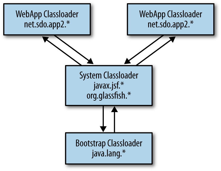
The net result is that when there is a request to load a class, the bootstrap
classloader is the first code that attempts to find the class; that is followed
by
the system (classpath) classloader, and then the
application-specific classloader(s). From a functional point of view, that’s
what makes sense: the bytecodes for the
java.lang.String
class must come from
the bootstrap classloader and not some other implementation that was
accidentally (or maliciously) included in some other classloader in the
hierarchy.
Prior to Java 7, the problem here was that the method to load the class was synchronized: only one classloader could delegate to the system classloader at a time. This drastically reduced any parallelization from using multiple classloaders, since each had to wait its turn for access into the system and bootstrap classloaders. Java 7 addresses that situation by using a set of locks based on the class name. Now, two classloaders that are looking for the same class will still contend for a lock, but classloaders that are looking for different classes can execute within the class hierarchy in parallel.
This benefit also applies if Java-supplied classloaders such
as the
URLClassLoader
are used. In Java 6, a URL classloader that was
the parent
of two (or more) addition classloaders would be a synchronization bottleneck
for parallel operations; in Java 7, the classloader is able to be used
in parallel. Java 7 supplied
classloaders are termed parallel-capable.
Classloaders are not parallel-capable by default. If you want to extend the benefits of parallel use into your own classloaders, you must take steps to make them parallel capable. There are two steps.
First, ensure that the classloader hierarchy does not contain any cycles. A cyclical classloader hierarchy is fairly uncommon. It also results in code that is quite difficult to maintain, since at some point in the cycle, some classloader must directly satisfy the request rather than passing the request to its parent classloader (else the delegation would have an infinite loop). So while it is technically possible to enable parallelism for a cyclical series of classloaders, it is a convoluted process (on top of already convoluted code). Since one precept of performant Java code is to employ common idioms and write simple code that the compiler can easily optimize, that case will not be recommended here.
Second, register the classloader as parallel-capable in a static initializer within the class:
publicclassMyCustomClassLoaderextendsSecureClassLoader{static{registerAsParallelCapable();}....}
This call must be made within each specific classloader implementation.
The
SecureClassLoader
is itself parallel capable, but subclasses do not pick up that setting.
If, within your own code, you have a second class that extends the
MyCustomClassLoader
class, that class must also register itself as parallel
capable.
For most classloaders, these are the only two steps that are required.
The recommended way to write a classloader is to override the
findClass()
method. Custom classloaders which instead override the
loadClass()
method
must also ensure that the
defineClass()
method is called only once for
each class name within each classloader instance.
As with all performance issues involving scalability around a lock, the net performance benefit of this optimization depends on how long the code in the lock is held. As a simple example, consider this code:
URLurl=newFile(args[0]).toURL();URLClassLoaderucl=newURLClassLoader(url);for(StringclassName:classNames){ucl.loadClass(className);}
The custom classloader here will look in a single jar file (passed on the
command line as the first element of
args).
Then it loops through an array of class names
(defined elsewhere) and loads each of the classes from that jar file.
The parent classloader here is the system classpath classloader. When two or more threads execute this loop concurrently, they will have to wait for each other as they delegate the lookup of the class into the classpath classloader. Table 12-2 shows the performance of this loop when the system classpath is empty.
| Number of Threads | Time in JDK 7 | Time in JDK 6 |
1 | 30.353 seconds | 27.696 seconds |
2 | 34.811 seconds | 31.409 seconds |
4 | 48.106 seconds | 72.208 seconds |
8 | 117.34 seconds | 184.45 seconds |
The time here is for 100 executions of the loop with a classname list of 1,500 classes. There are a few interesting conclusions to draw here. First, the more complex code in JDK 7 (to enable the parallel loading) has actually introduced a small penalty in the simplest case—an example of the principle that simpler code is faster. Even with two threads, the new model is slightly slower in this case, because the code spends virtually no time in the parent classloader: the time spent while the lock is held in the parent classloader is greatly outweighed by the time spent elsewhere in the program.
When there are four threads, things change. To begin, the four threads here are competing for CPU cycles against other processes on the four-CPU machine (in particular, there is a browser displaying a flash-enabled page, which is taking some 40% of a single CPU). So even in the JDK 7 case, the scaling isn’t linear. But at least the scaling is much better: in the JDK 6 case, there is now severe contention around the parent classloader lock.
There are two reasons for that contention. First, competition for the CPU has effectively increased the amount of time the classloader lock is held, and second, there are now twice as many threads competing for the lock.
Increasing the size of the system classpath also greatly increases the length of time the parent classloading lock is held. Table 12-3 repeats this experiment when the classpath has 266 entries (the number of jar files in the GlassFish distribution).[76]
| Number of Threads | Time in JDK 7 | Time in JDK 6 |
1 | 98.146 seconds | 92.129 seconds |
2 | 111.16 seconds | 316.01 seconds |
4 | 150.98 seconds | 708.24 seconds |
8 | 287.97 seconds | 1461.5 seconds |
Now, the contention even with only two threads is quite severe: without a parallel-enabled classloader, it takes three times longer to load the classes. And as load is injected into the already-stressed system, scaling becomes even worse. In the end, performance is as much as seven times slower.
There is an interesting trade-off here: whether to deploy the more
complex-code and slightly hurt performance in the single-threaded case, or
whether to optimize for other cases—particularly when, as in the last
example, the performance difference is quite large. These are the sort
of performance trade-offs that occur all the time, and in this case the
JDK team opted for the second choice as a default. As a platform, it is a
good idea to provide both choices (even though only one can be a default).
Hence, the JDK 6 behavior can be enabled by using the
-XX:+AlwaysLockClassLoader
flag (which is false by default). Long startup cycles without concurrent
threads loading classes from different classloaders may benefit slightly
from including that flag.
Quick Summary
- In complex applications (particularly application servers) with multiple classloaders, making those class loaders parallel-capable can solve issues where they are bottlenecked on the system or bootclass classloader.
- Applications that do a lot of classloading through a single classloader in a single thread may benefit from disabling the parallel-capable feature of Java 7.
Random numbers
Java 7 comes with three standard random-number generator classes:
java.util.Random,
java.util.concurrent.ThreadLocalRandom,
and
java.security.SecureRandom.
There are important performance differences among these three classes.
The difference between the
Random
and
ThreadLocalRandom
classes is that the main
operation (the
nextGaussian()
method) of the
Random
class
is synchronized. That method is used by any method that retrieves a random
value, so that lock can become contended no matter how the random number
generator is used:
if two threads use the same random number generator at the same
time, one will have to wait for the other to complete its operation. This
is why the thread-local version is used: when each thread has its own
random-number generator,
the synchronization of the
Random
class is no longer an issue.[77]
The difference between those classes and the
SecureRandom
class lies in the algorithm used.
The
Random
class (and the
ThreadLocalRandom
class, via inheritance) implement a
typical pseudo-random algorithm. While those
algorithms are quite sophisticated, they are—in the end—deterministic.
If the initial seed is known, it is easy to determine the exact
series of numbers the engine will generate. That means hackers are able to
look at series of numbers from a particular generator and (eventually)
figure out what the next number will be. Although good pseudo-random number
generators can emit series of numbers that look really random (and that
even fit probabilistic expectations of randomness), they are not truly random.
The
SecureRandom,
class, on the other hand, uses a system interface to obtain
random data. The way that data is generated is operating-system specific, but
in general this source provides data based on truly random events (such as when
the mouse is moved). This is known as entropy-based randomness and is much
more secure for operations that rely on random numbers. SSL encryption is the
best-known example of such an operation: the random numbers it uses for
encryption are impossible to determine with an entropy-based
source.[78]
Unfortunately, computers generate a limited amount of entropy, so it can take
a very long time to get a lot of random numbers from a secure random
number generator. Calls to the
nextRandom()
method of the
SecureRandom
class will take an
indeterminate amount of time, based on how much unused entropy the system
has. If no entropy is available, the call will appear to hang, possibly
as long as seconds at a time,
until the required entropy is available.
That makes performance timing quite difficult: the performance itself
becomes random.
This is often a problem for applications that create many SSL connections or otherwise need a lot of secure random numbers; it can take such applications a long time to perform their operations. When executing performance tests on such an application, be aware that the timings will have a very large amount of variance. There really isn’t any way to deal with that variance other than to run a huge number of sample tests as discussed in Chapter 2. The other alternative is to contact your operating system vendor and see if they have additional (or better) entropy-based sources available.
In a pinch, a third alternative to this problem is to run performance tests
using the
Random
class, even though the
SecureRandom
class will be used in production. If the performance tests are module-level
tests, that can make sense: those tests will need more random numbers (e.g.,
more SSL sockets) than the production system will need during the same period
of time. But eventually, the expected load must be tested with the
SecureRandom
class to determine if the load on the production system can obtain a sufficient
number of random numbers.
Quick Summary
-
Java’s default
Randomclass is expensive to initialize, but once initialized, it can be reused. -
In muti-threaded code, the
ThreadLocalRandomclass is preferred. -
The
SecureRandomclass will show arbitrary, completely random performance. Performance tests on code using that class must be carefully planned.
JNI
If you are interesting in writing the fastest possible code, avoid JNI.
Well-written Java code will run at least as fast on current versions of the JVM as corresponding C or C++ code (it is not 1996 anymore). Language purists will continue to debate the relative performance merits of Java and other languages, and there are doubtless examples you can find where an application written in another language is faster than the same application written in Java (though often, those examples contain poorly-written Java code). However, that debate misses the point of this section: when an application is already written in Java, calling native code for performance reasons is almost always a bad idea.
Still, there are times when JNI is quite useful. The Java platform provides many common features of operating systems, but if access to a special, operating-specific function is required, then so is JNI. And why build your own library to perform some operation, when a commercial (native) version of the code is readily available? In these and other cases, the question becomes how to write the most efficient JNI code.
The answer is to avoid making calls from Java to C as much as possible. Crossing the JNI boundary (the term for making the cross-language call), is quite expensive. Because calling an existing C library requires writing some glue code in the first place, take the time to create new, coarse-grained interfaces via that glue code: perform many, multiple calls into the C library in one shot.
Interesting, the reverse is not necessarily true: C code that calls back into Java does not suffer a large performance penalty (depending on the parameters involved). For example, consider the following code:
publicvoidmain(){calculateError();}publicvoidcalculateError(){for(inti=0;i<numberOfTrials;i++){error+=50-calc(numberOfIterations);}}publicdoublecalc(intn){doublesum=0;for(inti=0;i<n;i++){intr=random(100);// Return random value between 1 and 100sum+=r;}returnsum/n;}
This (completely nonsensical) code has two main loops—the inner loop makes
multiple calls to code that generates a random number, and the outer loop
repeatedly calls that inner loop to see how close to the expected value it
is. A JNI implementation could implement any subset of the
calculateError(),
calc(),
and
random()
methods in C. Table 12-4 shows the performance from
various permutations, given 10,000 trials.
| CalculateError | Calc | Random | JNI Transitions | Total Time |
Java | Java | Java | 0 | 12.4 seconds |
Java | Java | C | 10,000,000 | 32.1 seconds |
Java | C | C | 10,000 | 24.4 seconds |
C | Java | Java | 10,000 | 12.4 seconds |
C | C | C | 0 | 12.4 seconds |
Implementing only the inner-most method in JNI call provides the most
crossings of the JNI boundary (numberOfTrials * numberOfLoops, or
10 million). Reducing the number of crossings to numberOfTrails
(10,000) reduces that overhead substantially, and reducing it further to
0 provides the best performance—at least in terms of JNI, though
the pure Java implementation is just as fast as an
implementation that uses all native code.
JNI code performs worse if the parameters involved are not simple primitives.
Two aspects are involved in this overhead. First, for simple references, an
address translation is needed. This is one reason why, in the example above,
the call from Java to C experienced more overhead than the call from C to
Java: calls from Java to C implicitly pass the object in question (the
this
object) to the C function. The call from C to Java doesn’t pass any
objects.
Second, operations on array-based data are subject to special handling in
native code. This includes
String
objects, since the string data is
essentially a character array. To access the individual elements of these
arrays, a special call must be made to pin the object in memory (and
for
String
objects, to convert from Java’s UTF-16 encoding into UTF-8).
When the array is no longer needed, it must be explicitly released in the JNI
code. While the array is pinned, the garbage collector cannot run—so
one of the most expensive mistakes in JNI code is to pin a string or array
in code that is long-running. That prevents the garbage collector from running,
effectively blocking all the application threads until the JNI code
completes. It is extremely important to make the critical section
where the array is
pinned as short as possible.
Sometimes, this latter goal conflicts with the goal of reducing the calls which cross the JNI boundary. In that case, the latter goal is the more important one: even if it means making multiple crossings of the JNI boundary, make the sections that pin arrays and strings as short as possible.
Quick Summary
- JNI is not a solution to performance problems. Java code will almost always run faster than calling into native code.
- When JNI is used, limit the number of calls from Java to C; crossing the JNI boundary is expensive.
- JNI code that uses arrays or strings must pin those objects; limit the length of time they are pinned so that the garbage collector is not impacted.
Exceptions
Java exception processing has the reputation of being expensive. It is somewhat more expensive than processing regular control flows, though in most cases, the extra cost isn’t worth the effort to attempt to bypass it. On the other hand, because it isn’t free, exception processing shouldn’t be used as a general mechanism either. The guideline here is to use exceptions according to the general principles of good program design: mainly, code should only throw an exception to indicate something unexpected has happened. Following good code design means that your Java code will not be slowed down by exception processing.
Two things can affect the general performance of exception processing. First, there is the code block itself: is it expensive to set up a try-catch block? While that might have been the case a very long time ago, it has not been the case for years. Still, because the Internet has a long memory, you will sometimes see recommendations to avoid exceptions simply because of the try-catch block. Those recommendations are out of date; modern JVMs can generate code that handles exceptions quite efficiently.
The second aspect is that (most) exceptions involve obtaining a stack trace at the point of the exception. This operation can be expensive, particularly if the stack trace is deep.
Let’s look at an example. Here are three implementations of a particular method to consider:
publicArrayList<String>testSystemException(){ArrayList<String>al=newArrayList<>();for(inti=0;i<numTestLoops;i++){Objecto=null;if((i%exceptionFactor)!=0){o=newObject();}try{al.add(o.toString());}catch(NullPointerExceptionnpe){// Continue to get next string}}returnal;}publicArrayList<String>testCodeException(){ArrayList<String>al=newArrayList<>();for(inti=0;i<numTestLoops;i++){try{if((i%exceptionFactor)==0){thrownewNullPointerException("Force Exception");}Objecto=newObject();al.add(o.toString());}catch(NullPointerExceptionnpe){// Continue to get next string}}returnal;}publicArrayList<String>testDefensiveProgramming(){ArrayList<String>al=newArrayList<>();for(inti=0;i<numTestLoops;i++){Objecto=null;if((i%exceptionFactor)!=0){o=newObject();}if(o!=null){al.add(o.toString());}}returnal;}
Each method here returns an array of arbitrary strings from newly-created objects. The size of that array will vary, based on the desired number of exceptions to be thrown.
Table 12-5 shows the time to complete each method for 100,000
iterations given the worst case—an
exceptionFactor
of 1 (each iteration
generates an exception, and the result is an empty list). The example
code here is either shallow (meaning that the method in question is called
when there are only three classes on the stack), or deep (meaning that the
method in question is called when there are 100 classes on the stack).
| Method | Shallow Time | Deep Time |
Code Exception | 381 ms | 10673 ms |
System Exception | 15 ms | 15 ms |
Defensive Programming | 2 ms | 2 ms |
There are three interesting differences here. First, in the case where the code explicitly constructs an exception in each iteration, there is a significant difference of time between the shallow case and the deep case. Constructing that stack trace takes time—time that is dependent on the stack depth.
The second interesting difference is between the case where the code
explicitly creates the exception, and where the JVM creates the exception
when the null pointer is dereferenced (the first two lines in the table).
What’s happening is that
at some point, the compiler has optimized the
system-generated exception case—the JVM begins to reuse the same exception
object rather than creating a new one each time it is needed. That object
is reused each
time the code in question is executed, no matter what the calling stack is,
and the exception does not actually contain a call stack (i.e., the
printStackTrace()
method returns no output). This optimization doesn’t
occur until the full stack exception has been thrown for quite a long
time, so if your test case doesn’t include a sufficient warmup cycle, you will
not see its effects.
Finally, defensive programming provides the performance is the best yet. In this example, that isn’t surprising—it reduces the entire loop into a no-op. So take that number with a grain of salt.
Despite the differences between these implementations, notice that the overall time involved in most cases is quite small—on the order of milliseconds. Averaged out over 100,000 calls, the individual execution time differences will barely register (and recall that this is the worst-case example).
If the exceptions are used properly, then the number of exceptions in these loops will be quite small. Table 12-6 shows the time required to execute the loop 100,000 times generating 1,000 exceptions—1% of the time.
| Method | Shallow Time | Deep Time |
Code Exception | 56 ms | 157 ms |
System Exception | 51 ms | 52 ms |
Defensive Programming | 50 ms | 50 ms |
Now the processing time of the
toString()
method dominates the
calculation. There is still a penalty to pay for creating the exceptions
with deep stacks, but the benefit from testing for the
null
value in
advance has all but vanished.
So performance penalties for using exceptions injudiciously is smaller than
might be expected. Still, there are cases where you will run into code that
is simply creating too many exceptions. Since the performance penalty
comes from filling in the stack traces, the
-XX:-StackTraceInThrowable
flag (which is true by default) can be set to disable the generation
of the stack traces.
This is rarely a good idea—the reason the stack traces are present is to enable some analysis of what unexpectedly went wrong. That capability is lost when this flag is enabled. And there is code that actually examines the stack traces and determines how to recover from the exception based on what it finds there.[79] That’s problematic in itself, but the upshot is that disabling the stack trace can mysteriously break code.
There are some APIs in the JDK itself where exception handling can lead to
performance issues. Many collection classes will throw an exception when
non-existent items are retrieved from them. The
Stack
class, for example,
throws an
EmptyStackException
if the stack is empty when the
pop()
method
is called. It is usually better to utilize defensive programming in that
case by checking the stack length first.[80]
The most notorious example within the JDK of questionable use of
exceptions is in class loading: the
loadClass()
method of the
ClassLoader
class throws a
ClassNotFoundException
when
asked to load a class that it cannot find. That’s not actually an exceptional
condition. An individual classloader is not expected to know how to load
every class in an application, which is why there are hierarchies of
classloaders.
In an environment with dozens of class loaders, this means a lot of exceptions are created as the class loader hierarchy is searched for the one classloader that knows how to load the given class. The classloading example earlier in this chapter, for example, runs 3% faster when stack trace generation is disabled.
Still, that kind of difference is the exception more than the rule. That classloading example is a microbenchmark with a very long classpath, and even under those circumstances, the difference per call is on the order of a millisecond.
Quick Summary
- Exceptions are not necessarily expensive to process, though they should be used only when appropriate.
- The deeper the stack, the more expensive to process exceptions.
- The JVM will optimize away the stack penalty for frequently-created system exceptions.
- Disabling stack traces in exceptions can sometimes help performance, though crucial information is often lost in the process.
String Performance
Strings are central enough to Java that their performance has already been discussed in several other chapters. To highlight those cases:
- String Interning
- It is common to create many string objects that contain the same sequence of characters. These objects unnecessarily take space in the heap; since strings are immutable, it is often better to reuse the existing strings. See Chapter 7 for more details.
- String Encoding
-
While Java strings are UTF-16 encoded, most of the rest of the world uses a different encoding—so encoding of strings into different charsets is a common operation. The
encode()anddecode()methods of theCharsetclass are quite slow if they process only one (or a few) characters at a time; make sure that they are set up to process full buffers of data, as discussed earlier in this chapter. - Network Encoding
- Java EE application servers often have special handling for encoding static strings (from JSP files and so on); see Chapter 10 for more details.
String concatenation is another area where there are potential performance pitfalls. Consider a simple string concatenation like this:
Stringanswer=integerPart+"."+mantissa;
That code is actually quite performant; the syntactic sugar of
the javac compiler
turns that statement into this code:
Stringanswer=newStringBuilder(integerPart).append(".").append(mantissa).toString();
Problems arise, though, if the string is constructed piecemeal:
Stringanswer=integerPart;answer+=".";answer+=mantissa;
That code translates into:
Stringanswer=newStringBuilder(integerPart).toString();answer=newStringBuilder(answer).append(".").toString();answer=newStringBuilder(answer).append(mantissa).toString();
All those temporary
StringBuilder
and intermediate
String
objects are
inefficient. Never construct strings using concatenation unless it can
be done on a single (logical) line, and never use string concatenation
inside a loop
unless the concatenated string is not used on the next loop iteration.
Otherwise, always explicitly use a
StringBuilder
object
for better performance.[81]
Quick Summary
- One-line concatenation of strings yields good performance.
-
For multiple concatenation operations, make sure to use a
StringBuilder.
Logging
Logging is one of those things that performance engineers either love or hate—or (usually) both. Whenever I’m asked why a program is running badly, the first thing I ask for are any available logs, with the hope that logs produced by the application will have clues as to what the application was doing. Whenever I’m asked to review the performance of working code, I immediately recommend that all logging statements be turned off.
There are multiple logs in question here. Garbage collection produces its
own logging statements (see Chapter 6). That logging
can be directed into a distinct
file, the size of which can be managed by the JVM. Even in production code,
GC logging (with the
-XX:+PrintGCDetails
flag) has such low
overhead and such an expected large benefit if something goes wrong that
it should always be turned on.
Java EE application servers generate an access log that is updated on every request. This log generally has a noticeable impact: turning off that logging will definitely improve the performance of whatever test is run against the application server. From a diagnosability standpoint when something goes wrong, those logs are (in my experience) not terribly helpful. However, in terms of business requirements, that log is often crucial, in which case it must be left enabled.
Although it is not a Java EE standard, many
application servers support the apache mod_log_config standard which allows
you to specify exactly what information is logged for each request (and
servers which don’t follow the mod_log_config syntax will typically support
some other log customization). The key here is to log as little information
as possible and still meet the business requirements. The performance of the
log is subject to the amount of data written.
In HTTP access logs in particular (and in general, in any kind of log), it is a good idea to log all information numerically: IP addresses rather than host names, time stamps (e.g., seconds since the epoch) rather than string data (e.g., “Monday, June 3, 2013 17:23:00 -0600”), and so on. Minimize any data conversion which will take time and memory to compute so that the effect on the system is also minimized. Logs can always be post-processed to provide converted data.
There are three basic principles to keep in mind for application logs. First
is to keep a balance between the data to be logged and level at which it
is logged. There are seven standard logging levels in the JDK, and
loggers by default are configured to output three of those levels
(INFO
and greater).
This often leads to confusion within projects—INFO
level messages sound like
they should be fairly common and should provide a description of the flow
of an application (“now I’m processing task A”, “now I’m doing task B”, and
so on). Particularly for applications that are heavily threaded and scalable
(including Java EE application servers), that much logging will have
a detrimental effect on performance (not to mention running the risk of being
too chatty to be useful). Don’t be afraid to use the lower-level logging
statements.
Similarly, when code is checked into a group repository, consider the needs of the user of the project rather than your needs as a developer. We’d all like to have a lot of good feedback about how our code works once it is integrated into a larger system and run through a battery of tests, but if a message isn’t going to make sense to an end user or system administrator, it’s not helpful to enable it by default. It is merely going to slow down the system (and confuse the end user).
The second principle is to use fine-grained loggers. Having a logger per class can be tedious to configure, but having greater control over the logging output often makes this worthwhile. Sharing a logger for a set of classes in a small module is a good compromise. The point to keep in mind is that production problems—and particularly production problems that occur under load or are otherwise performance related—are tricky to reproduce if the environment changes significantly. Turning on too much logging often changes the environment such that the original issue no longer manifests itself.
Hence, you must be able to turn on logging
only for a small set of code (and, at least initially, a small set of logging
statements at the
FINE
level, followed by more at the
FINER
and
FINEST
levels) so that the performance of the code is not
affected.
Between these two principles, it should be possible to enable small subsets of messages in a production environment without affecting the performance of the system. That is usually a requirement anyway: the production system administrators probably aren’t going to enable logging if it slows the system down, and if the system does slow down, then the likelihood of reproducing the issue is reduced.
The third principle to keep in mind when introducing logging into code is
to remember that it is quite easy to write logging code that has unintended
side-effects, even if the logging is not enabled. This is another case where
“prematurely” optimization code is a good thing—as the example from
Chapter 1 shows, remember to use the
isLoggable()
method anytime
the information to be logged contains a method call, a string concatenation,
or any other sort of allocation (for example, allocation of an
Object
array for a
MessageFormat
argument).
Quick Summary
- Code should contain lots of logging to enable users to figure out what it does, but none of that should be enabled by default.
- Don’t forget to test for the logging level before calling the logger if the arguments to the logger require method calls or object allocation.
Java Collections API
Java’s collections API is quite extensive; there are at least 58 different collection classes supplied by Java 7. Using an appropriate collection class—as well as using collection classes appropriately—is an important performance consideration in writing an application.
The first rule in using a collection class is to use one suitable for the
algorithmic needs of an application. This advice is not specific to Java;
it is in essentially Data Structures 101. A
LinkedList
is not suitable
for searching; if access to a random piece of data is required, store the
collection in a
HashMap.
If the data needs to remain sorted, use a
TreeMap
rather than attempting to sort the data in the application. Use an
ArrayList
if the data will be accessed by index, but not if data frequently needs to
be inserted into the middle of the array. And so on…the algorithmic choice
of which collection class is crucial, but the choice in Java isn’t different
than the choice in any other programming language.
There are, however, some idiosyncrasies to consider when using Java collections.
Synchronized vs. Unsynchronized
By default, virtually all Java collections are unsynchronized (the major
exceptions being the
Hashtable,
Vector,
and their related classes).
Chapter 9 posited a microbenchmark to compare CAS-based protection to traditional synchronization. That proved to be impractical in the threaded case, but what if the data in question will only ever be accessed by a single thread—what would be the effect of not using any synchronization at all? Table 12-7 shows that comparison. Because there is no attempt to model the contention, the microbenchmark in this case is valid in this one circumstance—when there can be no contention, and the question at hand is what the penalty is for “over-synchronizing” access to the resource.
| Mode | Total Time | Per-Operation Time |
CAS Operation | 6.6 seconds | 13 nanoseconds |
Synchronized Method | 11.8 seconds | 23 nanoseconds |
Unsynchronized Method | 3.9 seconds | 7.8 nanoseconds |
The second column makes it clear that there is small a penalty when using any data protection technique as opposed to simple unsynchronized access. However, keep in mind this is a microbenchmark executing 500 million operations—so the difference in time-per-operation is on the order of 15 nanoseconds. If the operation in question is executed frequently enough in the target application, the performance penalty will be somewhat noticeable. In most cases, the difference will be outweighed by far larger inefficiencies in other areas of the application. Remember also that the absolute number here is completely determined by the target machine the test was run on (my home machine with a 4-core AMD Athlon); to get a more realistic measurement, the test would need to be run on hardware that is the same as the target environment.
So, given a choice between a synchronized
Vector
and an unsynchronized
ArrayList,
which should be used? Access to the
ArrayList
will be
slightly faster, and depending how often the list is accessed, there can
be a measurable performance difference here.[82]
On the other hand, this assumes that the code will never be accessed by more than one thread. That may be true today, but what about tomorrow? If that might change, then it is better to use the synchronized collection now and mitigate any performance impact that results. This is a design choice, and whether future-proofing code to be threadsafe is worth the time and effort will depend on the circumstances of the application being developed.
If the choice is between using an unsynchronized collection and a
collection using CAS principles (e.g., a
HashMap
compared to a
ConcurrentHashMap),
then the performance difference is
even less important. CAS-based classes show virtually no overhead when used
in an uncontended environment (though keep reading for a discussion
of memory differences
in the particular case of hash maps).
Collection Sizing
Collection classes are designed to hold an arbitrary number of data elements and to expand as necessary as new items are added to the collection. There are two performance considerations here.
Although the data types provided by collection classes in Java are quite rich,
at a basic level those classes must hold their data using only Java
primitive data types: numbers (integers, doubles, and so on),
object references, and arrays of those types. Hence, an
ArrayList
of
String
objects contains an actual array:
privatetransientObject[]elementData;
As items are added and removed from the
ArrayList
they are stored at the
desired location within the
elementData
array (possibly causing other
items in the array to shift). Similarly, a
HashMap
contains an array of
an internal data type called
HashMap$Entry,
which maps each key/value pair
to a location in the array specified by the hashcode of the key.
Not all collections use an array to hold their elements; a
LinkedList
for example, holds each data element in an internally-defined
Node
class.
But collection classes that do use an array to hold their elements are
subject to special sizing considerations. You can tell if a particular
class falls into this category by looking at its constructors: if it has
a constructor that allows the initial size of the collection to be specified,
then it is internally using some array to store the items.
For those collection classes, it is important to accurately
specifying the initial size.
Take the simple example of an
ArrayList:
the
elementData
array will (by default) start out with an initial size of 10. When
the 11th item is inserted into an
ArrayList,
the list must expand the
elementData array.
This means allocating a new array, copying the original contents
into that array, and then adding in the new item. The data structure and
algorithm used by, say, the
HashMap
class is much more complicated, but
the principle is the same: at some point, those internal structures must be
resized.
The
ArrayList
class chooses to resize the array by adding roughly half
of the existing size, so the size of the
elementData
array will first
be 10, then 15, then 22, then 33, and so on. Whatever algorithm is used to
resize the array (see sidebar), this results in some wasted memory (which
in turn will affect the time the application spends performance GC).
Additionally, each time the array must be resized, an expensive array
copy operation must occur to transfer the contents from the old array to
the new array.
To minimize those performance penalties, make sure to construct the collection with as accurate an estimate of the ultimate size of the collection whenever possible.
Collections and Memory Efficiency
We’ve just seen one example where the memory efficiency of collections can be sub-optimal: there is often some wasted memory in the backing store used to hold the elements in the collection.
This can be particularly problematic for sparsely-used collections: those with one or two elements in them. These sparsely-used collections can waste a large amount of memory if they are used extensively. One way to deal with that is to size the collection when it is created. Another way is to consider if a collection is really needed in that case at all.
When most developers are asked how to quickly sort any array, they will offer up quicksort as the answer. Good performance engineers will want to know the size of the array: if the array is small enough, then the fastest way to sort it will be to use insertion sort.[83] Size matters.
Similarly, a
HashMap
is the fastest way to look up items based on some
key value—but if there is only one key, then the
HashMap
is overkill
compared to using a simple object reference. Even if there are a few keys,
maintaining a few object references will consume much less memory than a
full
HashMap
object, with the resulting (positive) effect on GC.
Along those lines, one important difference to know regarding the
memory use of collection classes
is the difference in size between a
HashMap
object, and a
ConcurrentHashMap
object. Prior to Java 7, the size of an empty or sparsely-populated
ConcurrentHashMap
object was quite large: over 1K (even when a small size was passed to the
constructor). In Java 7, that size is only 208 bytes
(compared to 128 bytes for an empty
HashMap
constructed without a specified size,
and 72 bytes for a
HashMap
constructed with a size of one).
This size difference can still be important in applications where there is
a proliferation of small maps, but the optimizations made in Java 7 make
that difference much less significant. There are existing performance
recommendations (including some by me) that urge avoiding the
ConcurrentHashMap
class in applications where memory is important and
the number
of maps is large. Those recommendations center around the trade-off of
possible faster access to the map (if it is contended) against the increased
pressure on the garbage collector the larger maps cause. That trade-off
still applies, but the balance is now much more in favor
of using the
ConcurrentHashMap.
Quick Summary
- Carefully consider how collections will be accessed and choose the right type of synchronization for them. However, the penalty for uncontended access to a memory-protected collection (particularly one using CAS-based protections) is minimal; sometimes it is better to be safe than sorry.
- Sizing of collections can have a large impact on performance: either slowing down the garbage collector if the collection is too large, or causing lots of copying and resizing if it is to small.
AggressiveOpts
The
AggressiveOpts
flag (by default, false) affects the behavior of several basic Java SE operations.
The purpose of this flag is to introduce optimizations on a trial basis;
over time, the optimizations enabled by this flag can be expected to become the
default setting for the JVM. Many of those optimizations that were
experimented with in Java 6 have already become the default in
Java 7u4. You should re-test this flag with every release of the JDK to see if it is still
positively affecting your application.
Alternate Implementations
The major effect of enabling the
AggressiveOpts
flag is that it substitutes different implementations for several basic JDK classes—notably, the
BigDecimal,
BigInteger,
and MutableBigDecimal classes
from the
java.math package;
the
DecimalFormat,
DigitalList
and NumberFormat classes
from the
java.text package;
and the
HashMap,
LinkedHashMap, and
TreeMap classes
from the
java.util package.
These classes are functionally the same as the classes in the standard JDK that they replace, but they have more efficient implementations. In Java 8, these alternate implementations have been removed—either they have been incorporated into the base JDK classes, or the base JDK classes have been improved in other ways.
The reason that these classes are
enabled (in Java 7) only when the
AggressiveOpts
flag is set is because their behavior can trigger subtle bugs in application code. For
example, the aggressive implementation of the HashMap class yields an iterator that
returns the keys in a different order than the standard implementation. Applications should
never depend on the order of items returned from this iterator in the first place, but
it turns out that many applications made that mistake. For compatibility reasons, then,
the more efficient implementation did not override the original implementation, and it
is necessary to set the
AggressiveOpts
flag to get the better implementation.
Since Java 8 removes these classes, the bug-compatibility they preserve may break when upgrading—which is an indication to write better code in the first place.
Miscellaneous Flags
Enabling the
AggressiveOpts
flag affects some other minor tunings of the JVM.
Settings the
AggressiveOpts
flag enables the
AutoFill
flag, which
be default is false in JDK 7 though 7u4, when the default is set to true.
That flag enables some
better loop optimizations by the compiler. Similarly, this flag also enables the
DoEscapeAnalysis
flag (that is also set by default in JDK 7u4 and later versions).
The
AutoBoxCacheMax
flag (default 128) is set to 20,000—that enables more vales to be autoboxed, which can
slightly improve performance for certain applications (at the expense of using slightly more
memory). The value of the
BiasedLockingStartupDelay
is reduced from its
default of 2000 to 500, meaning that biased locking will start sooner after the application
begins execution.
Finally, this flag enables the
OptimizeStringConcat
flag, which allows the JVM to optimize the use of StringBuilder objects—in particular,
the StringBuilder objects that are created (by the javac compiler) when writing code like
this:
String s = obj1 + ":" + obj2 + ":" + obj3;
The javac compiler translates that code into a series of append() calls on a string builder.
When the
OptimizeStringConcat
flag is enabled, the JVM just-in-time compiler can optimize away the creation of the
StringBuilder
object itself. The
OptimizeStringConcat
flag is false by default in JDK 7 until 7u4, when the default becomes true.
Quick Summary
-
The
AggressiveOptsflag enables certain optimizations in base classes. For the most part, these classes are faster than their replacements, but they may have unexpected side effects. - These classes have been removed in Java 8.
Lambdas and Anonymous Classes
For many developers, the most exciting feature of Java 8 is the addition of lambdas. There is no denying that lambdas have a hugely positive performance impact on the productivity of Java developers, though of course that benefit is difficult to quantify. But we can examine the performance of code using lambda constructs.
The most basic question about the performance of lambdas is how they compare to their replacement—anonymous classes. There turns out to be little difference.
The usual example of how to use a lambda class begins with code that creates anonymous inner classes:.[84]
privatevolatileintsum;publicinterfaceIntegerInterface{intgetInt();}publicvoidcalc(){IntegerInterfacea1=newIntegerInterface(){publicintgetInt(){return1;}};IntegerInterfacea2=newIntegerInterface(){publicintgetInt(){return2;}};IntegerInterfacea3=newIntegerInterface(){publicintgetInt(){return3;}};sum=a1.get()+a2.get()+a3.get();}
That is compared to the following code using lambdas:
publicvoidcalc(){IntegerInterfacea3->{return3};IntegerInterfacea2->{return2};IntegerInterfacea1->{return1};sum=a3.get()+a2.get()+a1.get();}
The body of the lambda or anonymous class is crucial here—if that body performs any significant operations, then the time spent in the operation is going to overwhelm any small difference in the implementations of the lambda or the anonymous class. However, even in this minimal case, the time to perform this operation is essentially the same, as Table 12-8 shows.
calc() method using lambdas and anonymous classes.| Implementation | Time in microseconds |
Anonymous Classes | 87.2 |
Lambda | 87.9 |
Numbers always look impressively official, but we can’t conclude anything from
this other than that the performance of the two implementations is basically
equivalent. That’s true because of the random variations in tests, but also because
these calls are measured using
System.nanoTime().
Timing simply isn’t accurate enough to believe at that level; what we do
know is that for all intents and purposes, this performance is the same.
One interesting thing about the typical usage in this example is that the code that uses the anonymous class creates a new object every the method is called. If the method is called a lot (as of course if must be in a benchmark to measure its performance), many instances of that anonymous class are quickly created and discarded. As we saw in Chapter 5, that kind of usage has very little impact on performance. There is a very small cost to allocate (and, more important, initialize) the objects, and because they are discarded quickly they do not really slow down the garbage collector.
Nonetheless, cases can be constructed where that allocation matters and where it is better to reuse those objects:
privateIntegerInterfacea1=newIntegerInterface(){publicintgetInt(){return1;}};...Similarlyfortheotherinterfaces....publicvoidcalc(){returna1.get()+a2.get()+a3.get();}}
The typical usage of the lambda does not create a new object on each iteration of the loop—making this an area where some corner cases can favor the performance of the lambda usage. Nonetheless, it is difficult to construct even microbenchmarks where these differences matter.
Lambda and Anonymous Classloading
One corner case where this difference does come into play is in startup and class loading. It is tempting to look at the code for a lambda and conclude that it is syntactic sugar around creating an anonymous class (particularly since, in the long run, their performance is equal). But that is not how it works—the code for a lambda creates a static method that is called through a special helper class in JDK 8. The anonymous class is an actual Java class—it has a separate class file and will be loaded from the classloader.
As we saw previously in this chapter, classloading performance can be important,
particularly if there is a long classpath. If this example is run such that
every execution of the
calc()
method is performed in a new classloader, the anonymous class implementation is
at a disadvantage.
calc() method in a new classloader| Implementation | Time in microseconds |
Anonymous Classes | 267 |
Lambdas | 181 |
One point about these numbers—they are after a suitable warmup period to allow for compilation. But one other thing that happens during the warmup period is that the class files are read from disk for the first time. The OS will keep those files in memory (in the OS filesystem buffers). So the very first execution of the code will take much longer, as the calls to the OS to read the files will actually load them from disk. Subsequent calls will be faster—they will still call the OS to read the files, but since the files are in the OS memory, their data is returned quickly. So the result for the anonymous class implementation is better than it might otherwise be, since it doesn’t include any actual disk reading of the class files.
Quick Summary
- The choice between using a lambda or an anonymous class should be dictated by ease of programming, since there is no difference between their performance.
- Lambdas are not implemented as classes, so one exception to that rule is in environments where classloading behavior is important; lambdas will be slightly faster in that case.
Stream and Filter Performance
One other key feature of Java 8, and one that is frequently used in conjunction
with lambdas, is the new
Stream
facility. One very important performance feature of streams is that they can
automatically parallelize code. Information about parallel streams can
be found in
Chapter 9; this section discusses some general performance
features of streams and filters.
Lazy Traversal
The first performance benefit from streams is that they are implemented as
lazy data structures. Consider the example where we have a list of stock
symbols, and the goal is to find the first symbol in the list that does not
contain the letter A. The code to do that through a stream looks like this:
publicStringfindSymbol(ArrayList<String>al){Optional<String>t=al.stream().filter(symbol->symbol.charAt(0)!='A').filter(symbol->symbol.charAt(1)!='A').filter(symbol->symbol.charAt(2)!='A').filter(symbol->symbol.charAt(3)!='A').findFirst();returnt.get();}
There’s obviously a better way to implement this using a single filter, but
we’ll save that discussion for later. For now, consider what it means for the
stream to be implemented lazily in this example. Each
filter()
method returns a new stream, so there are in effect four logical streams here.
The
filter()
method, it turns out, doesn’t really do anything except set up a series of
pointers. The effect of that is when the
findFirst()
method is invoked on the stream, no data processing has been performed—no
comparisons of data to the character A have yet been made.
Instead, the
findFirst()
asks the previous stream (returned from filter 4) for an element. That stream
has no elements yet, so it calls back to the stream produced by filter 3, and
so on. Filter 1 will grab the first element from the array list (from the
stream, technically) and test to see if its first character is A. If so, it
completes the callback and returns that element downstream; otherwise, it
continues to iterate through the array until it finds a matching element (or
exhausts the array). Filter 2 behaves similarly—when the callback to filter
1 returns, it tests to see if the second character is A. If so, it completes
its callback and passes the symbol downstream; if not, it makes another callback
to filter 1 to get the next symbol.
All those callbacks may sound inefficient, but consider the alternative. An algorithm to process the streams eagerly would look something like this:
private<T>ArrayList<T>calcArray(ArrayLisr<T>src,Predicate<T>p){ArrayList<T>dst=newArrayList<>();for(Ts:src){if(p.test(s))dst.add(s);}returndst;}privatestaticlongcalcEager(ArrayList<String>a1){longthen=System.currentTimeMillis();ArrayList<String>a2=calcArray(a1,(Strings)->s.charAt(0)!='A');ArrayList<String>a3=calcArray(a2,(Strings)->s.charAt(1)!='A');ArrayList<String>a4=calcArray(a3,(Strings)->s.charAt(2)!='A');ArrayList<String>a5=calcArray(a4,(Strings)->s.charAt(3)!='A');answer=a5.get(0);longnow=System.currentTimeMillis();returnnow-then;}
There are two reasons this alternative is less efficient than the lazy
implementation that Java actually adopted. First, it requires the creation
of a lot of temporary instances of the
ArrayList
class. Second, in the lazy implementation, processing can stop as soon as
the
findFirst()
method gets an element. That means only a subset of the items must actually
pass through the filters. The eager implementation, on the other hand, must
process the entire list several times until the last list is created.
Hence, it should come as no surprise that the lazy implementation is far
more performant than the alternative in this example. In this case, the
test is processing a list of 456,976 four-letter symbols, which are sorted
in alphabetical order. The eager implementation
processes only 18,278 of those before it encounters the symbol BBBB,
at which point it can stop. It takes the iterator two orders of magnitude longer
to find that answer:
| Implementation | Seconds |
Filter/findFirst | 0.359 |
Iterator/findFirst | 48.706 |
One reason, then, why filters can be so much faster than iterators is simply that they can take advantage of algorithmic opportunities for optimizations: the lazy filter implementation can end processing whenever it has done what it needs to do, processing less data.
What if the entire set of data must be processed—what is the basic performance of filters vs. iterators in that case? For this example, we’ll change the test slightly. The previous example made a good teaching point about how multiple filters worked, but hopefully it was obvious that the code would perform better with a single filter:
publicintcountSymbols(ArrayList<String>al){intcount=0;t=al.stream().filter(symbol->symbol.charAt(0)!='A'&&symbol.charAt(1)!='A'&&symbol.charAt(2)!='A'&&symbol.charAt(3)!='A').forEach(symbol->count++);returncount;}
The example here also changes the final code to count the symbols so that the entire list will be processed. On the flip side, the eager implementation can now use an iterator directly:
publicintcountSymbols(ArrayList<String>al){intcount=0;for(Stringsymbol:al){if(symbol.charAt(0)!='A'&&symbol.charAt(1)!='A'&&symbol.charAt(2)!='A'&&symbol.charAt(3)!='A')count++;returncount;}
Even in this case, the lazy filter implementation is faster than the iterator:
| Implemementation | Time Required |
Multiple Filters | 18.0 seconds |
Single Filter | 6.5 seconds |
Iterator/count | 6.8 seconds |
For comparison sake, Table 12-11 includes (as its first line) the case where the entire list is processed using four separate filters as opposed to the optimal case: one filter, which is slightly faster even than an iterator.
Quick Summary
- Filters offer a very significant performance advantage by allowing processing to end in the middle of iterating through the data.
- Even when the entire data set if processed, a single filter will slightly outperform an iterator.
- Multiple filters have some overhead; make sure to write good filters.
Summary
This look into some key areas of the Java SE JDK concludes
our examination of Java performance. One interesting theme to most of
the topics of this chapter is that they show the the evolution of the
performance of the JDK itself. As Java developed and matured as a platform,
its developers discovered that repeatedly-generated exceptions didn’t need
to spend time providing thread stacks; that using a threadlocal variable to
avoid synchronization of the random number generator was a good thing; that
the default size of a
ConcurrentHashMap
was too large; that classloaders
were not able to run in parallel due to a synchronization lock; and so on.
This continual process of successive improvement is what Java performance tuning is all about. From tuning the compiler and garbage collector, to using memory effectively, to understanding key performance differences in the SE and EE APIs and more, the tools and processes in this book will allow you to provide similar on-going improvements in your own code.
[76] GlassFish doesn’t simply put all those files into a single classloader; it has been chosen here simply as an expedient example.
[77] As discussed in Chapter 7, the thread-local version also provides significant performance benefits because it is reusing an expensive-to-create object.
[78] There are other ways to break encryption methods for data,
even when a SecureRandom random number generator is used in the algorithm.
[79] The reference implementation of CORBA works like that.
[80] On the other hand, unlike
many collection classes, the Stack class supports null objects, so
it’s not as if the pop() method could return null to indicate an empty
stack.
[81] In Chapter 1, I argued that there are times to “prematurely” optimize when that phrase is used in a context meaning simply “write good code.” This is a prime example.
[82] As noted in Chapter 9, excessive calls to the synchronized method can be quite painful for performance on certain hardware platforms as well.
[83] Algorithms
based on quicksort will usually use insertion sort for small arrays anyway;
in the case of Java, the implementation of the Arrays.sort() method assumes
that any array with less than 47 elements will be sorted faster with
insertion sort than with quicksort.
[84] The usual example often uses a Stream
rather than the iterator shown here. Information about the Stream class comes later in
this section.