
Chapter 6. Garbage Collection Algorithms
Chapter 5 examined the general behavior of all garbage collectors, including JVM flags that apply universally to all GC algorithms: how to select heap sizes, generation sizes, logging, and so on.
The basic tunings of garbage collection suffice for many circumstances. When they do not, it is time to examine the specific operation of the GC algorithm in use to determine how its parameters can be changed in order to minimize the impact of garbage collection on the application.
The key information needed to tune an individual collector is the data from the GC log when that collector is enabled. This chapter starts, then, by looking at each algorithm from the perspective of its log output—that allows us to understand how the GC algorithm works, and how it can be adjusted to work better. Each section then includes tuning information to achieve that better performance.
There are a few unusual cases that impact the performance of all garbage collection algorithms—allocation of very large objects, objects that are neither short- nor long-lived, and so on. Those cases are covered at the end of this chapter.
Understanding the Throughput Collector
We’ll start by looking at the individual garbage collectors, beginning with the throughput collector. The throughput collector has two basic operations: it collects the young generation, and it collects the old generation.
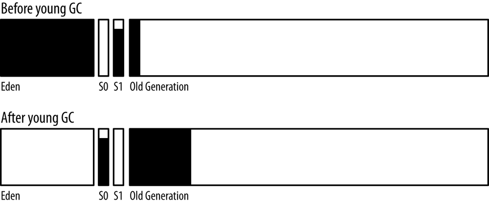
Figure 6-1 shows the heap before and after a young collection.
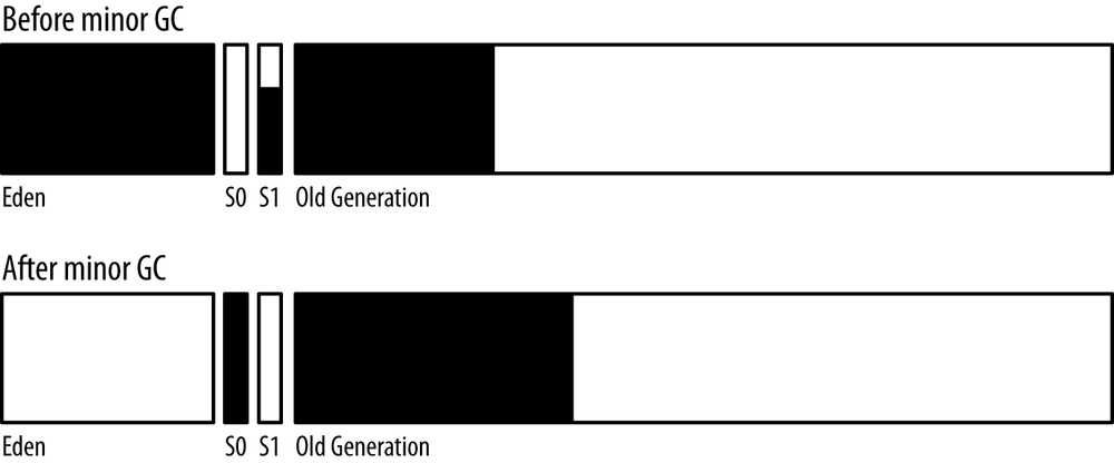
A young collection occurs when eden has filled up. The young collection moves all objects out of eden: some are moved to one of the survivor spaces (S0 in this diagram) and some are moved to the old generation, which now contains more objects. Many objects, of course, are discarded because they are no longer referenced.
In the
PrintGCDetails
GC log, a minor GC appears like this:
17.806: [GC [PSYoungGen: 227983K->14463K(264128K)]
             280122K->66610K(613696K), 0.0169320 secs]
             [Times: user=0.05 sys=0.00, real=0.02 secs]
This GC occurred 17.806 seconds after the program began. Objects in the young generation now occupy 14463 KB (14MB, in the survivor space); before the GC, they occupied 227983 KB (227 MB).[27] The total size of the young generation at this point is 264 MB.
Meanwhile the overall occupancy of the heap (both young and old generations) decreased from 280 MB to 66 MB, and the size of the entire heap at this point in time was 613 MB. The operation took less than 0.02 seconds (the 0.02 seconds of real time at the end of the output is 0.0169320 seconds—the actual time—rounded). The program was charged for more CPU time than real time because the young collections was done by multiple threads (in this configuration, four threads).
Figure 6-2 shows the heap before and after a full GC.
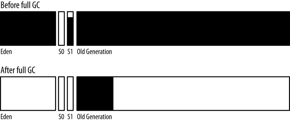
The old collection frees everything out of the young generation (including from the survivor spaces). The only objects that remain in the old generation are those which have active references, and all of those objects have been compacted so that the beginning of the old generation is occupied, and the remainder is free.
The GC log reports that operation like this:
64.546: [Full GC [PSYoungGen: 15808K->0K(339456K)]
          [ParOldGen: 457753K->392528K(554432K)] 473561K->392528K(893888K)
          [PSPermGen: 56728K->56728K(115392K)], 1.3367080 secs]
          [Times: user=4.44 sys=0.01, real=1.34 secs]
The young generation now occupies 0 bytes (and its size is 339 MB). The data in the old generation decreased from 457 MB to 392 MB, and hence the entire heap usage has decreased from 473 MB to 392 MB. The size of permgen is unchanged; it is not collected during most full GCs.[28] Because there is substantially more work to do in a full GC, it has taken 1.3 seconds of real time, and 4.4 seconds of CPU time (again for four parallel threads).
Quick Summary
- The throughput collector has two operations: minor collections and full GCs.
- Timings taken from GC log are a quick way to determine the overall impact of GC on an application using the throughput collector.
Adaptive and Static Heap Size Tuning
Tuning the throughput collector is all about pause times and striking a balance between the overall heap size and the sizes of the old and young generations.
There are two trade-offs to consider here. First, there is the classic programming trade-off of time vs. space. A larger heap consumes more memory on the machine, and the benefit of consuming that memory is (at least to a certain extent) that the application will have a higher throughput.
The second trade-off concerns the length of time it takes to perform GC. The number of full GC pauses can be reduced by increasing the heap size, but that may have the perverse effect of increasing average response times because of the longer GC times. Similarly, full GC pauses can be shortened by allocating more of the heap to the young generation than to the old generation, but that in turn increases the frequency of the old GC collections.
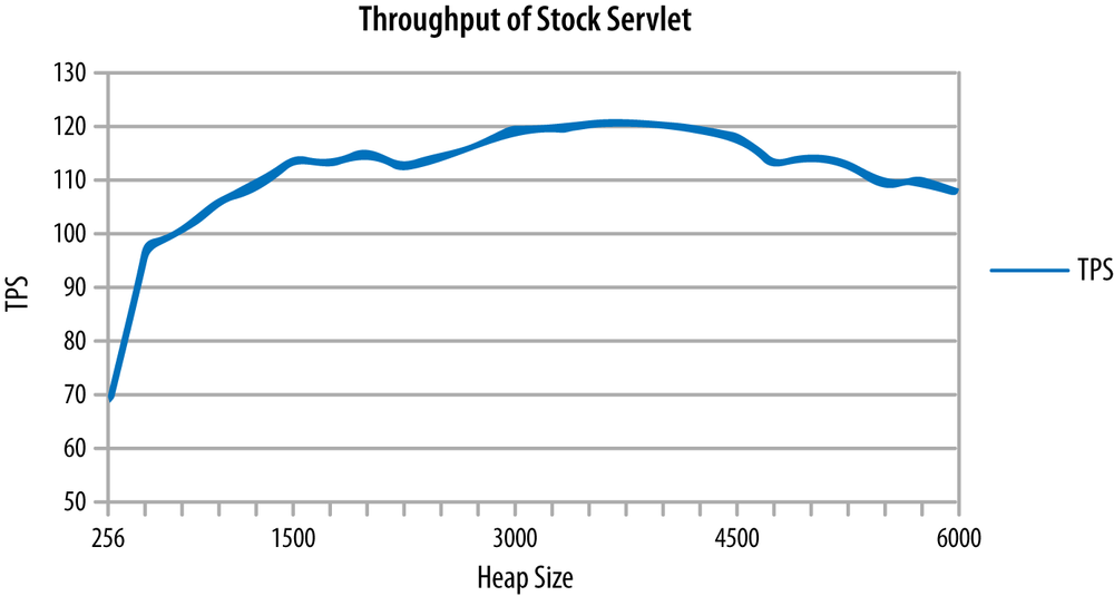
The effect of these trade-offs is shown in Figure 6-3. This graph shows the maximum throughput of the stock servlet application running in a Glassfish instance with different heap sizes. With a small 256 MB heap, the application server is spending quite a lot of time in GC (36% of total time, in fact); the throughput is restricted as a result. As the heap size is increased, the throughput rapidly increases—until the heap size is set to 1500 MB. After that, throughput increases less rapidly—the application isn’t really GC-bound at that point (about 6% of time in GC). The law of diminishing returns has crept in here: the application can use additional memory to gain throughput, but the gains become more limited.
After a heap size of 4500 MB, the throughput starts to decrease slightly. At that point, the application has reached the second trade-off: the additional memory has caused much longer GC cycles, and those longer cycles—even though they are less frequent—can impact the overall throughput.
The data in this graph was obtained by disabling adaptive sizing in the JVM—the minimum and maximum heaps sizes were set to the same value. It is possible to run experiments on any application and determine the best sizes for the heap and for the generations, but it is often easier to let the JVM make those decisions (which is what usually happens, since adaptive sizing is enabled by default).
Adaptive sizing in the throughput collector
will resize the heap (and the generations) in order
to meet its pause time goals. Those goals are set with these
flags:
-XX:MaxGCPauseMillis=N
and
-XX:GCTimeRatio=N.
The
MaxGCPauseMillis
flag specifies the maximum pause
time that the application is willing to tolerate. It might be
tempting to set this
to 0, or perhaps some very small value like 50 ms. Be aware that this goal
applies to both minor and full GCs. If a very small value is used,
the application will end up with a very small old generation: e.g., one that
can be cleaned in
50 ms. That will cause the JVM will perform very, very frequent
full GCs, and performance will be dismal.
So be realistic: set the value to
something that can actually be achieved. By default, this flag is not set.
The
GCTimeRatio
flag specifies the amount of time you are willing for the application to
spend in GC (compared to the amount of time its application-level threads
should run).
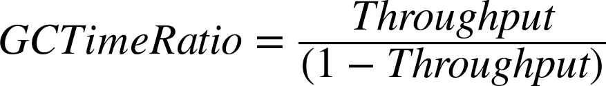
It is a ratio, so the value for N takes a little thought.
The value is used in the following equation to determine the percentage
of time the application threads should ideally run:

The default value for
GCTimeRatio
is 99. Plugging that value into the equation yields 0.99, meaning that the
goal is to spend 99% of time in application processing, and
only 1% of time in GC. But don’t be confused by how those numbers line up
in the default case. A
GCTimeRatio
of 95 does not mean that GC should run up to 5% of the time: it means
that GC should run up to 1.94% of the time.
I find it easier to decide what percentage of time
I’d like the application to spend performing useful work (say, 95%),
and then calculate the value of the
GCTimeRatio
from this equation:
For a throughput goal of 95% (0.95), this equation yields a
GCTimeRatio
of 19.
The JVM uses these two flags to set the size of the heap within the
boundaries established by the initial (-Xms) and maximum (-Xmx) heap
sizes. The
MaxGCPauseMillis
flag takes precedence: if it is set, the
sizes of the young and old generation are adjusted until the pause time
goal is met. Once that happens, the overall size of the heap is increased
until the time ratio goal is met. Once both goals are met, the JVM will
attempt to reduce the size of the heap so that it ends up with the
smallest-possible heap that meets these two goals.
Because the pause time goal is not set by default, the usual effect of
automatic heap sizing is that
the heap (and generation) sizes will increase until the
GCTimeRatio
goal is met. In practice, though, the default setting of that
flag is quite optimistic. Your experience will vary,
of course, but I am much more used to seeing applications that spend 3% - 6%
of their time in GC and behave quite well. Sometimes I even work on severely
applications in environments where they must use smaller heaps than are
optimal; those applications end up spending 10-15% of their time in GC.
GC has a substantial
impact on the performance of those application, but the
overall performance goals are still met.
So the best setting will vary depending on the application goals. In the absence of other goals, I start with a time ratio of 19 (5% of time in GC).
Table 6-1 shows the effects of this dynamic tuning for an application that needs a small heap and does little garbage collection (it is the stock servlet running in Glassfish where no session state is saved, and there are very few long-lived objects).
| GC Settings | End Heap Size | Percent time in GC | Ops/sec |
Default | 649MB | 0.9% | 9.2 |
MaxGCPauseMillis=50ms | 560MB | 1.0% | 9.2 |
Xms=Xmx=2048m | 2GB | 0.04% | 9.2 |
By default, the heap will have a 64 MB minimum size and a 2 GB maximum
size (since the machine has 8 GB of physical memory). In that case,
the
GCTimeRatio
works just as expected: the heap dynamically resized to 649 MB, at which
point the application was spending about 1% of total time in GC.
Setting the
MaxGCPauseMillis
in this case starts to reduce the size of the heap in order to meet that
pause time goal. Because there is so little work for the garbage collector
to perform in this example, it succeeds and can still spend only 1% of
total time in GC, while maintaining the same throughput of 9.2 ops/second.
Finally, notice that more isn’t always better—a full 2 GB heap does mean that the application can spend less time in GC, but GC isn’t the dominant performance factor here, and so the throughput doesn’t increase. As usual, spending time optimizing the wrong area of the application does has not helped.
If the same application is changed but the previous 50 requests for each user are saved in the session state, the garbage collector has to work harder. Table 6-2 shows the trade-offs in that situation.
| GC Settings | End Heap Size | Percent time in GC | Ops/sec |
Default | 1.7GB | 9.3% | 8.4 |
MaxGCPauseMillis=50ms | 588MB | 15.1% | 7.9 |
Xms=Xmx=2048m | 2GB | 5.1% | 9.0 |
Xmx=3560M;MaxGCRatio=19 | 2.1GB | 8.8% | 9.0 |
In a test that spends a significant amount of time in GC, things are different. The JVM will never be able to satisfy the 1% throughput goal in this test; it tries its best to accommodate the default goal and does a reasonable job, utilizing 1.7GB of space.
Things are worse when an unrealistic pause time goal is given. To achieve a 50 ms collection time, the heap is kept to 588 MB, but that means that GC now becomes excessively frequent. Consequently, the throughput has decreased significantly. In this scenario, the better performance comes from instructing the JVM to utilize the entire heap by setting the both the initial and maximum sizes to 2 GB.
Finally, the last line of the table shows what happens when the heap is reasonably sized and we set a realistic time ratio goal of 5%. The JVM itself determined that approximately 2 GB was the optimal heap size, and it achieved the same throughput as the hand-tuned case.
Quick Summary
- Dynamic heap tuning is a good first step for heap sizing. For a wide set of applications, that will be all that is needed, and the dynamic settings will minimize the JVM’s memory use.
- It is possible to statically size the heap to get the maximum possible performance. The sizes the JVM determines for a reasonable set of performance goals are a good first start for that tuning.
Understanding the CMS Collector
CMS has three basic operations:
- CMS collects the young generation (stopping all application threads)
- CMS runs a concurrent cycle to clean data out of the old generation
- If necessary, CMS performs a full GC
A CMS collection of the young generation appears in Figure 6-4.
A CMS young collection is very similar to a throughput young collection: data is moved from eden into one survivor space and into the old generation.
The GC log entry for CMS is also similar:
89.853: [GC 89.853: [ParNew: 629120K->69888K(629120K), 0.1218970 secs]
                1303940K->772142K(2027264K), 0.1220090 secs]
                [Times: user=0.42 sys=0.02, real=0.12 secs]
The size of the young generation is presently 629 MB; after collection, 69 MB of it remains (in a survivor space). Similarly, the size of the entire heap is 2027 MB, 772 MB of which is occupied after the collection. The entire process took 0.12 seconds, though the parallel GC threads racked up 0.42 seconds in CPU usage.
A concurrent cycle is shown in Figure 6-5.
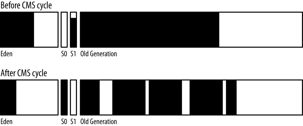
The JVM starts a concurrent cycle based on the occupancy of the heap. When it is sufficiently full, the JVM starts background threads which cycle through the heap and remove objects. At the end of the cycle, the heap looks like the bottom row in this diagram. Notice that the old generation is not compacted—there are areas where objects are allocated, and free areas. When a young collection moves objects from eden into the old generation, the JVM will attempt to use those free areas to hold the objects.
In the GC log, this cycle appears as a number of phases. Although a majority of the concurrent cycle uses background threads, some phases introduce short pauses where all application threads are stopped.
The concurrent cycle starts with an initial mark phase, which stops all the application threads:
89.976: [GC [1 CMS-initial-mark: 702254K(1398144K)]
                772530K(2027264K), 0.0830120 secs]
                [Times: user=0.08 sys=0.00, real=0.08 secs]
This phase is responsible for finding all the GC root objects in the heap. The first set of numbers shows that objects currently occupy 702 MB of 1398 MB of the old generation, while the second set shows that the occupancy of the entire 2027 MB heap is 772 MB. The application threads were stopped for a period of 0.08 seconds during this phase of the CMS cycle.
The next phase is the mark phase, and it does not stop the application threads. The phase is represented in the GC log by these lines:
90.059: [CMS-concurrent-mark-start]
90.887: [CMS-concurrent-mark: 0.823/0.828 secs]
                [Times: user=1.11 sys=0.00, real=0.83 secs]
The mark phase took 0.83 seconds (and 1.11 seconds of CPU time). Since it is just a marking phase, it hasn’t done anything to the heap occupancy, and so no data is shown about that. If there were data, it would likely show a growth in the heap from objects allocated in the young generation during those 0.83 seconds, since the application threads have continued to execute.
Next comes a preclean phase, which also runs concurrently with the application threads:
90.887: [CMS-concurrent-preclean-start]
90.892: [CMS-concurrent-preclean: 0.005/0.005 secs]
                [Times: user=0.01 sys=0.00, real=0.01 secs]
The next phase is a remark phase, but it involves several operations:
90.892: [CMS-concurrent-abortable-preclean-start]
92.392: [GC 92.393: [ParNew: 629120K->69888K(629120K), 0.1289040 secs]
                1331374K->803967K(2027264K), 0.1290200 secs]
                [Times: user=0.44 sys=0.01, real=0.12 secs]
94.473: [CMS-concurrent-abortable-preclean: 3.451/3.581 secs]
                [Times: user=5.03 sys=0.03, real=3.58 secs]

94.474: [GC[YG occupancy: 466937 K (629120 K)]
        94.474: [Rescan (parallel) , 0.1850000 secs]
        94.659: [weak refs processing, 0.0000370 secs]
        94.659: [scrub string table, 0.0011530 secs]
                [1 CMS-remark: 734079K(1398144K)]
                1201017K(2027264K), 0.1863430 secs]
        [Times: user=0.60 sys=0.01, real=0.18 secs]
Wait, didn’t CMS just execute a preclean phase? What’s up with this abortable preclean phase?
The abortable preclean phase is used because the the remark phase (which, strictly speaking, is the final entry in this output) is not a concurrent phase—it will stop all the application threads. CMS wants to avoid the situation where a young generation collection occurs and is immediately followed by a remark phase, in which case the application threads would be stopped for two back-to-back pause operations. The goal here is to minimize pause lengths by preventing back-to-back pauses.
Hence, the abortable preclean phase waits until the young generation is about 50% full. In theory, that is halfway between young generation collections, giving CMS the best chance to avoid those back-to-back pauses. In this example, the abortable pre-clean phase starts at 90.8 seconds and waits about 1.5 seconds for the regular young collection to occur (at 92.392 seconds into the log). CMS uses past behavior to calculate when the next young collection is likely to occur—in the case, it calculated it would occur in about 4.2 seconds. So after 2.1 seconds (at 94.4 seconds), CMS ends the pre-clean phase (which it calls “aborting” the phase, even though that is the only way the phase is stopped). Then, finally, CMS executes the remark phase, which pauses the application threads for 0.18 seconds (the application threads were not paused during the abortable pre-clean phase).
Next comes another concurrent phase—the sweep phase:
94.661: [CMS-concurrent-sweep-start]
95.223: [GC 95.223: [ParNew: 629120K->69888K(629120K), 0.1322530 secs]
                999428K->472094K(2027264K), 0.1323690 secs]
                [Times: user=0.43 sys=0.00, real=0.13 secs]
95.474: [CMS-concurrent-sweep: 0.680/0.813 secs]
                [Times: user=1.45 sys=0.00, real=0.82 secs]
This phase took 0.82 seconds and ran concurrently with the application threads. It also happened to be interrupted by a young collection. This young collection had nothing to do with the sweep phase, but it is left in here as an example that the young collections can occur simultaneously with the old collection phases. In Figure 6-5, notice that the state of the young generation changed during the concurrent collection—there may have been an arbitrary number of young collections during the sweep phase (and there will have been at least one young collection because of the abortable pre-clean phase).
Next comes the concurrent reset phase:
95.474: [CMS-concurrent-reset-start]
95.479: [CMS-concurrent-reset: 0.005/0.005 secs]
        [Times: user=0.00 sys=0.00, real=0.00 secs]
That is the last of the concurrent phases; the CMS cycle is now complete, and the unreferenced objects found in the old generation are now free (resulting in the heap shown in Figure 6-5). Unfortunately, the log doesn’t provide any information about how many objects were freed; the reset line doesn’t give any information about the heap occupancy. To get an idea of that, look to the the next young collection, which is:
98.049: [GC 98.049: [ParNew: 629120K->69888K(629120K), 0.1487040 secs]
                1031326K->504955K(2027264K), 0.1488730 secs]
Now compare the occupancy of the old generation at 89.853 seconds (before the CMS cycle began), which was roughly 703 MB (the entire heap occupied 772 MB at that point, which included 69 MB in the survivor space, so the old generation consumed the remaining 703 MB). In the collection at 98.049 seconds, the old generation occupies about 504 MB; the CMS cycle therefore cleaned up about 199 MB of memory.
If all goes well, these are the only cycles that CMS will run and the only log messages that will appear in the CMS GC log. But there are three more messages to look for, which indicate that CMS ran into a problem. The first is a concurrent-mode failure:
267.006: [GC 267.006: [ParNew: 629120K->629120K(629120K), 0.0000200 secs]
        267.006: [CMS267.350: [CMS-concurrent-mark: 2.683/2.804 secs]
        [Times: user=4.81 sys=0.02, real=2.80 secs]
        (concurrent mode failure):
        1378132K->1366755K(1398144K), 5.6213320 secs]
        2007252K->1366755K(2027264K),
        [CMS Perm : 57231K->57222K(95548K)], 5.6215150 secs]
        [Times: user=5.63 sys=0.00, real=5.62 secs]
When a young collection occurs and there isn’t enough room in the old generation to hold all the objects that are expected to be promoted, CMS executes what is essentially a full GC. All application threads are stopped, and the old generation is cleaned of any dead objects, reducing its occupancy to 1366 MB—an operation which kept the application threads paused for a full 5.6 seconds. That operation is single-threaded, which is one reason it takes so long (and one reason why concurrent mode failures are worse as the heap grows).
The second problem occurs when there is enough room in the old generation to hold the promoted objects, but the free space is fragmented and so the promotion fails:
6043.903: [GC 6043.903:
        [ParNew (promotion failed): 614254K->629120K(629120K), 0.1619839 secs]
        6044.217: [CMS: 1342523K->1336533K(2027264K), 30.7884210 secs]
        2004251K->1336533K(1398144K),
        [CMS Perm : 57231K->57231K(95548K)], 28.1361340 secs]
        [Times: user=28.13 sys=0.38, real=28.13 secs]
Here, CMS started a young collection and assumed that there was enough free space to hold all the promoted objects (otherwise, it would have declared a concurrent-mode failure). That assumption proved incorrect: CMS couldn’t promote the objects because the old generation was fragmented (or, much less likely, because the amount of memory to be promoted was bigger than CMS expected).
As a result, in the middle of the young collection (when all threads are already stopped), CMS collected and compacted the entire old generation. The good news is that with the heap compacted, fragmentation issues are solved (at least for a while). But that came with a hefty 28-second pause time. This time is much longer than when CMS had a concurrent-mode failure because the entire heap is compacted; the concurrent-mode failure simply freed objects in the heap. The heap at this point appears as it did at the end of the throughput collector’s full GC (Figure 6-2): the young generation is completely empty, and the old generation has been compacted.
Finally, the CMS log may show a full GC without any of the usual concurrent GC messages:
279.803: [Full GC 279.803:
                [CMS: 88569K->68870K(1398144K), 0.6714090 secs]
                558070K->68870K(2027264K),
                [CMS Perm : 81919K->77654K(81920K)],
                0.6716570 secs]
This occurs when permgen has filled up and needs to be collected; notice that the size of the CMS Perm space has dropped. In Java 8, this can also occur if the metaspace needs to be resized. By default, CMS does not collect permgen (or the metaspace), so if it fills up, a full GC is needed to discard any unreferenced classes. The advanced tuning section for CMS shows how to overcome this issue.
Quick Summary
- CMS has several GC operations, but the expected operations are minor GCs and concurrent cycles.
- Concurrent mode failures and promotion failures in CMS are quite expensive; CMS should be tuned to avoid those as much as possible.
- By default, CMS does not collect permgen.
Tuning to solve Concurrent Mode Failures
The primary concern when tuning CMS is to make sure that there are no concurrent mode or promotion failures. As the CMS GC log showed, a concurrent mode failure occurs because CMS did not clean out the old generation fast enough: when it comes time to perform a collection in the young generation, CMS calculates that it doesn’t have enough room to promote those objects to the old generation and instead collects the old generation first.
The old generation initially fills up by placing the objects right next to each other. When some amount of the old generation is filled (by default, 70%), the concurrent cycle begins and the background CMS thread(s) start scanning the old generation for garbage. At this point, a race is on: CMS must complete scanning the old generation and freeing objects before the remaining (30%) of the old generation fills up. If the concurrent cycle loses the race, CMS will experience a concurrent-mode failure.
There are multiple ways to attempt to avoid this failure:
- Make the old generation larger, either by shifting the proportion of the new generation to the old generation, or by adding more heap space altogether.
- Run the background thread more often.
- Use more background threads.
If more memory is available, the better solution is to increase the size of the heap. Otherwise, change the way the background threads operate.
Running the background thread more often
One way to let CMS win the race is to start the concurrent cycle sooner.
If the concurrent cycle starts when 60% of the old generation is filled,
CMS has a better chance
of finishing than if the cycle starts when 70% of the old generation is filled.
The easiest way to achieve that is to set both these flags:
-XX:CMSInitiatingOccupancyFraction=N
and
-XX:+UseCMSInitiatingOccupancyOnly.
Using
both those flags also makes CMS easier to understand: if they are both set,
then CMS determines when to start the background thread based only on the
percentage of the old generation that is filled.
By default, the
UseCMSInitiatingOccupancyOnly
flag is false, and CMS uses a more complex algorithm to determine when
to start the background thread. If the background thread needs to be started
earlier, better to start it the simplest way possible and set the
UseCMSInitiatingOccupancyOnly
flag to true.
Tuning the value of the
CMSInitiatingOccupancyFraction
may require a few iterations. If
UseCMSInitiatingOccupancyOnly
is enabled, then the default value for
CMSInitiatingOccupancyFraction
is 70: the CMS cycle starts when the old generation is 70%
occupied.
A better value for that flag for a given application can be found in the GC log by figuring out when the failed CMS started in the first place. Find the concurrent mode failure in the log, and then look back to when the most recent CMS cycle started. The CMS-intial-mark line will show how full the old generation was when the CMS cycle started.
89.976: [GC [1 CMS-initial-mark: 702254K(1398144K)]
                772530K(2027264K), 0.0830120 secs]
                [Times: user=0.08 sys=0.00, real=0.08 secs]
In this example, that works out to about 50% (702 MB
out of 1398 MB). That was not soon enough, so the
CMSInitiatingOccupancyFraction
needs to be set to something lower than 50.[29]
The temptation here is just to set the value to 0 or some other small number so that the background CMS cycle runs all the time. That’s usually discouraged, but as long as you aware of the trade-offs being made, it may work out fine.
The first trade-off comes in CPU time: the CMS background thread(s) will run continually, and they consume a fair amount of CPU—each background CPU thread will consume 100% of a CPU. There will also be very short bursts when multiple CMS threads run and the total CPU on the box spikes as a result. If these threads are running needlessly, that is wasteful of CPU resources.
On the other hand, it isn’t necessarily a problem to use those CPU cycles. The background CMS threads have to run sometimes, even in the best case. Hence, the machine must always have enough CPU cycles available to run those CMS threads. So when sizing the machine, you must plan for that CPU usage.
Could those CPU cycles be used for something else when the CMS background thread isn’t running? Not usually. If another application uses those cycles, it has no way of knowing when the CMS thread is running. As a result, the other application and the CMS thread will compete for CPU, which will make the CMS thread more likely to lose its race. Sophisticated operating system tuning can sometimes be used to run those competing applications with a priority that ensures the CMS thread takes precedence, but that can be tricky to get right. So yes: when CMS cycles run too frequently, far more CPU cycles are used, but those CPU cycles would otherwise just be idle.
The second trade-off is far more significant and has to do with pauses. As the GC log showed, certain phases of the CMS cycle stop all the application threads. The main reason CMS is used is to limit the effect of GC pauses, and so running CMS more often than needed is counter-productive. The CMS pauses are generally much shorter than a young generation pause, and a particular application may not be sensitive to those additional pauses—it’s a trade-off between the additional pauses and the reduced chance of a concurrent-mode failure. But continually running the background GC pauses will likely lead to excessive overall pauses, which will in the end ultimately reduce the performance of the application.
Unless those trade-offs are acceptable, take care not
to set the
CMSInitiatingOccupancyFraction
higher than the amount of live
data in the heap, plus at least 10-20%.
Adjusting the CMS background threads
Each CMS background thread will consume 100% of a CPU on a machine.
If an application experiences a concurrent mode failure and there are extra
CPU cycles available,
the number of those background threads can be increased by setting the
-XX:ConcGCThreads=N
flag. By default, that value is set based on the
value of the
ParallelGCThreads
flag:
ConcGCThreads = (3 + ParallelGCThreads) / 4
This calculation is performed using integer arithmetic, which means
there will be one
ConcGCThread
for up to four
ParallelGCThreads;
then
two
ConcGCThreads
for between five and eight
ParallelGCThreads,
and so on.
The key to tunings this flag is whether there are available CPU cycles. If the
number of
ConcGCThreads
is set too high, they will take CPU cycles away
from the application threads; in effect, small pauses will be introduced into
the program as the application threads wait for their chance run on the CPU.
Alternately, on a system with lots of CPUs,
the default value of
ConcGCThreads
may be too high. If concurrent mode failures are not occurring, the
number of those threads can often be reduced in order to save CPU cycles.
Quick Summary
- Avoiding concurrent mode failures is the key to achieving the best possible performance with CMS.
- The simplest way to avoid those failures (when possible) is to increase the size of the heap.
-
Otherwise, the next step is to start the concurrent background threads sooner by adjusting the
CMSInitiatingOccupancyFraction. - Tuning the number of background threads can also help.
Tuning CMS for Permgen
The example CMS GC log showed a full GC caused when permgen needed to be collected (and the same thing can happen if the metaspace needs to be resized). This will happen most frequently for developers who are continually (re)deploying applications to an application server, or to any other such application that frequently defines (and discards) classes.
By default, the CMS threads in Java 7 do not process permgen, and so if permgen
fills up, CMS executes a full GC to collect it. Alternately,
the
-XX:+CMSPermGenSweepingEnabled
flag can be enabled (it is false by default), so that permgen is
collected just like the old generation: by a set of background thread(s)
concurrently sweeping permgen.
Note that the trigger
to perform this sweeping is independent of the old generation. CMS
permgen collection occurs when the occupancy ratio of permgen hits the value
specified by
-XX:CMSInitiatingPermOccupancyFraction=N,
which
defaults to 80%.
Enabling permgen sweeping is only part of the story, though—to actually
free the unreferenced classes, the flag
-XX:+CMSClassUnloadingEnabled
must be set. Otherwise, the CMS permgen sweeping will
manage to free a few miscellaneous objects, but no class metadata will be
freed. Since the bulk of the data
in permgen is that class metadata, this flag should always be used when
CMS permgen sweeping is enabled.
In Java 8, CMS does clean unloaded classes from the metaspace by default.
If for some reason
you wanted to disable that, unset the
-XX:-CMSClassUnloadingEnabled flag (by default, it is true).
Incremental CMS
This chapter has continually stressed the fact that extra CPU is needed in order to run CMS effectively. What if you have only a single CPU machine, but still need a low-pause collector? Or have multiple, but very busy, CPUs?
In those cases, CMS can be set so that it operates incrementally, which means that when the background thread runs (and there should never be more than one such thread), it doesn’t sweep through the entire heap at once. Having that background thread pause periodically will help overall throughput by making more CPU available to the application thread(s). When it does run, though, the application threads and the CMS thread will still compete for CPU cycles.
Incremental CMS is enabled by specifying the
-XX:+CMSIncrementalMode
flag. The rate at which the background thread yields to the
application threads is controlled by changing the values of the
-XX:CMSIncrementalSafetyFactor=N,
-XX:CMSIncrementalDutyCycleMin=N,
and
-XX:-CMSIncrementalPacing
flags.
Incremental CMS operates on the principal of a duty cycle, which governs how long the CMS background thread will scan the heap before yielding time to the application threads. At the operating system level, the background thread is already competing with (and will be time-sliced with) the application threads. These flags instead control how long the background thread will run before voluntarily stopping for a while in order to let the application threads run.
The duty cycle is calculated in terms of the length of time between collections of the young generation; by default, incremental CMS will be allowed to run for 20% of that time (at least to start, though CMS will adjust that value in order to try and keep pace with the amount of data promoted to the old generation). If that isn’t long enough, concurrent mode failures (and full GCs) will occur; the goal here is to tune incremental CMS to avoid (or at least minimize) those GCs.
Start by increasing the
CMSIncrementalSafetyFactor,
which is the percent
of time added to the default duty cycle. The default duty cycle value starts
at 10%, and the safety factor is, by default, an additional 10% (yielding the
default 20% initial duty cycle). To give the background thread more time to run,
try increasing the safety factor (up to a maximum of 90—which will cause
the incremental cycle to run 100% of the
time).
Alternately, adjust the duty cycle directly by setting the
CMSIncrementalDutyCycleMin
value to a number greater than its default
value (10). However, this value is subject to automatic adjustment by the JVM
as it monitors the amount of data promoted to the old generation. So even
if that number is increased, the JVM may decide on its own that
the incremental CMS doesn’t need to run that often and hence it may decrease
that value. If an application has bursts in its operation, that
calculation will frequently be incorrect, and you will need to both set the
duty cycle explicitly and also disable the adjustment of that value by
turning off the
CMSIncrementalDutyCycle
flag (which is true by default).
Quick Summary
- Incremental CMS is useful when an application needs low pause times but is running on a machine with limited CPU resources.
- Incremental CMS is controlled via a duty cycle; lengthening the duty cycle can help to avoid concurrent mode failures with CMS.
Understanding the G1 Collector
G1 is a concurrent collector that operates on discrete regions within the heap. Each region (there are by default around 2048 of them) can belong to either the old or new generation, and the generational regions need not be contiguous. The idea behind having regions in the old generation is that when the concurrent background threads look for unreferenced objects, some regions will contain more garbage than other regions. The actual collection of a region still requires that application threads be stopped, but G1 can focus on the regions that are mostly garbage and only spend a little bit of time emptying those regions. This approach—clearing out only the mostly garbage regions—is what gives G1 its name: Garbage First.
That doesn’t apply to the regions in the young generation—during a young GC, the entire young generation is either freed or promoted (to a survivor space or to the old generation). Still, the young generation is defined in terms of regions, in part because it makes resizing the generations much easier if the regions are pre-defined.
G1 has four main operations:
- A young collection.
- A background, concurrent cycle.
- A mixed collection.
- If necessary, a full GC.
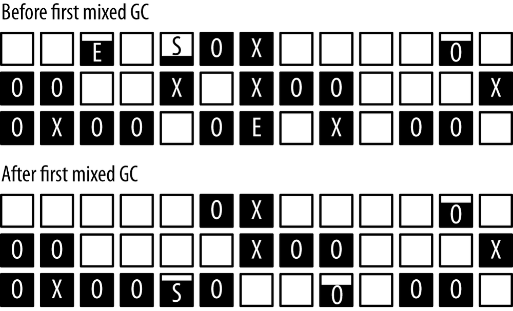
We’ll look at each of those in turn, starting with the G1 young collection shown in Figure 6-6.
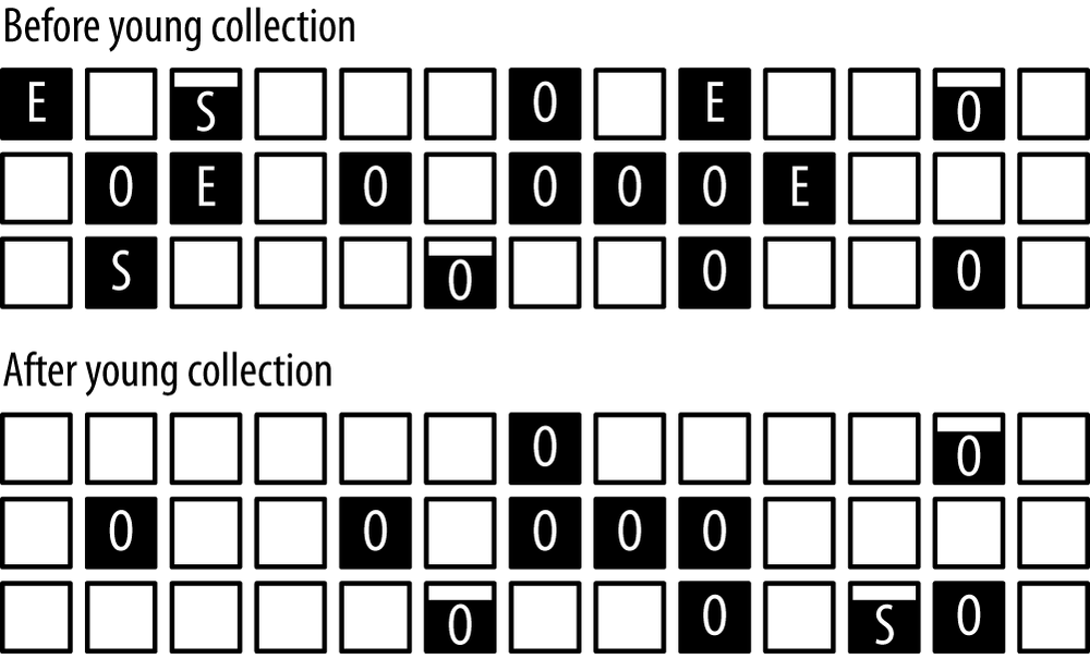
Each small square in this figure represents a G1 region. The data in each region is represented by the black area of the region, and the letter in each region identifies the generation to which the region belongs ([E]den, [O]ld generation, [S]urvivor space). Empty regions do not belong to a generation; G1 uses them arbitrarily for whichever generation it deems necessary.
The G1 young collection is triggered when eden fills up (in this case, after filling four regions). After the collection, there are no regions assigned to eden, since it is empty. There is at least one region assigned to the a survivor space (partially filled in this example), and some data has moved into the old generation. In this example, very little data was promoted from eden into the old generation—what data was promoted filled part of an old generation region in the bottom row of the diagram.
The GC log illustrates this collection a little differently in G1 than in
other collectors.
As usual, the example log was taken using
PrintGCDetails,
but the details in the
log for G1 are more verbose. The examples show
only a few of the
important lines.
Here is the standard collection of the young generation:
23.430: [GC pause (young), 0.23094400 secs]
...
   [Eden: 1286M(1286M)->0B(1212M)
        Survivors: 78M->152M Heap: 1454M(4096M)->242M(4096M)]
   [Times: user=0.85 sys=0.05, real=0.23 secs]
Collection of the young generation took .23 seconds of real time, during which the GC threads consumed .85 seconds of CPU time. 1286 MB of objects were moved out of eden (which was resized to 1212 MB); 74 MB of those moved to the survivor space (it increased in size from 78 M to 152 MB) and the rest were freed. We know they were freed by observing that the total heap occupancy decreased by 1212 MB. In the general case, some objects from the survivor space might have been moved to the old generation, and if the survivor space were full, some objects from eden would have been promoted directly to the old generation—in those cases, the size of the old generation will increase.
A concurrent G1 cycle begins and ends as shown in Figure 6-7.
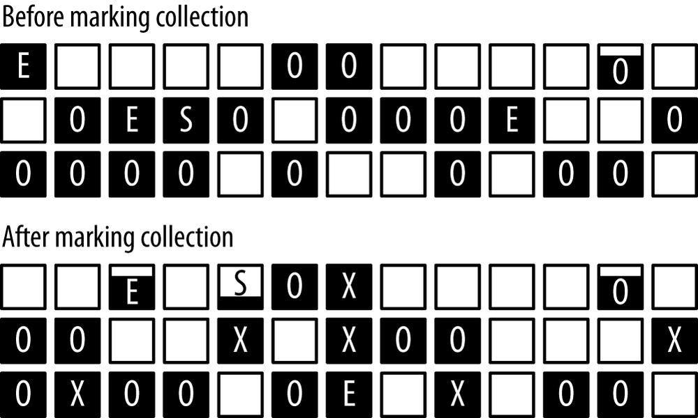
The are three important things to observe in this diagram. First, the young generation has changed its occupancy—there will be at least one (and possibly more) young collections during the concurrent cycle. Hence, the eden regions before the marking cycle have been completely freed, and new eden regions have started to be allocated.
Second, some regions are now marked with an X. Those regions belong to the old generation (and note that they still contain data)—they are regions that the marking cycle has determined contain mostly garbage.
Finally, notice that the old generation (consisting of the regions marked with an O or an X) is actually more occupied after the cycle has completed. That’s because the young generation collections that occurred during the marking cycle promoted data into the old generation. In addition, the marking cycle doesn’t actually free any data in the old generation: it merely identifies regions that are mostly garbage. Data from those regions is freed in a later cycle.
The G1 concurrent cycle has several phases, some of which stop all application threads and some of which do not. The first phase is an initial-mark phase. That phase stops all application threads—partly because it also executes a young collection:
50.541: [GC pause (young) (initial-mark), 0.27767100 secs]
    [Eden: 1220M(1220M)->0B(1220M)
        Survivors: 144M->144M Heap: 3242M(4096M)->2093M(4096M)]
    [Times: user=1.02 sys=0.04, real=0.28 secs]
As in a regular young collection, the application threads were stopped (for .28 seconds), and the young generation was emptied (71 MB of data was moved from the young generation to the old generation). The initial-mark output announces that the background concurrent cycle has begun. Since the initial mark phase also requires all application threads to be stopped, G1 takes advantage of the young GC cycle to do that work. The impact of adding the initial mark phase to the young GC wasn’t that large: it used 20% more CPU cycles than the previous collection, even though the pause was only slightly longer.[30]
Next, G1 scans the root region:
50.819: [GC concurrent-root-region-scan-start]
51.408: [GC concurrent-root-region-scan-end, 0.5890230]
This took .58 seconds, but it doesn’t stop the application threads; it only uses the background threads. However, this phase cannot be interrupted by a young collection, so having available CPU cycles for those background threads is crucial. If the young generation happens to fill up during the root region scanning, the young collection (which has stopped all the application threads) must wait for the root scanning to complete. In effect, this means a longer-than-usual pause to collect the young generation. That situation is shown in the GC log like this:
350.994: [GC pause (young)
        351.093: [GC concurrent-root-region-scan-end, 0.6100090]
        351.093: [GC concurrent-mark-start],
        0.37559600 secs]
The GC pause here starts before the end of the root region scanning, which (along with the interleaved output) indicates that it was waiting. The time stamps show that application threads waited about 100ms—which is why the duration of the young GC pause is about 100ms longer than the average duration of other pauses in this log.[31]
After the root region scanning, G1 enters a concurrent marking phase. This happens completely in the background; a message is printed when it starts and ends:
111.382: [GC concurrent-mark-start]
....
120.905: [GC concurrent-mark-end, 9.5225160 sec]
Concurrent marking can be interrupted, so young collections may occur during this phase. The marking phase is followed by a remarking phase and a normal cleanup phase:
120.910: [GC remark 120.959:
        [GC ref-PRC, 0.0000890 secs], 0.0718990 secs]
        [Times: user=0.23 sys=0.01, real=0.08 secs]
120.985: [GC cleanup 3510M->3434M(4096M), 0.0111040 secs]
        [Times: user=0.04 sys=0.00, real=0.01 secs]
These phases stop the application threads, though usually for a quite short time. Next there is an additional cleanup phase which happens concurrently:
120.996: [GC concurrent-cleanup-start]
120.996: [GC concurrent-cleanup-end, 0.0004520]
And with that, the normal G1 cycle is complete—insofar as finding the garbage goes, at least. But very little has actually been freed yet. A little memory was reclaimed in the cleanup phase, but all G1 has really done at this point is to identify old regions that are mostly garbage and can be reclaimed (the ones marked with an X in Figure 6-7).
Now G1 executes a series of mixed GCs. They are called mixed because they perform the normal young collection, but they also collect some number of the marked regions from the background scan. The effect of a mixed GC is shown in Figure 6-8.
As is usual for a young collection, G1 has completely emptied eden and adjusted the survivor spaces. Additionally, two of the marked regions have been collected. Those regions were known to contain mostly garbage, and so a large part of them was freed. Any live data in those regions was moved to another region (just like live data was moved from the young generation into regions in the old generation). This is why G1 ends up with a fragmented heap less often than CMS—moving the objects like this is compacting the heap as G1 goes along.
The mixed GC operation looks like this in the log:
79.826: [GC pause (mixed), 0.26161600 secs]
....
   [Eden: 1222M(1222M)->0B(1220M)
        Survivors: 142M->144M Heap: 3200M(4096M)->1964M(4096M)]
   [Times: user=1.01 sys=0.00, real=0.26 secs]
Notice that the entire heap usage has been reduced by more than just the 1222 MB removed from eden. That difference (16 MB) seems small, but remember that some of the survivor space was promoted into the old generation at the same time; in addition, each mixed GC cleans up only a portion of the targeted old generation regions. As we continue, we’ll see that it is important to make sure that the mixed GCs clean up enough memory to prevent future concurrent failures.
The mixed GC cycles will continue until (almost) all of the marked regions have been collected, at which point G1 will resume regular young GC cycles. Eventually, G1 will start another concurrent cycle to determine which regions should be freed next.
As with CMS, there are times when you’ll observe a full GC in the log, which is an indication that more tuning (including, possibly, more heap space) will benefit the application performance. There are primarily four times when this is triggered:
- Concurrent Mode Failure
G1 starts a marking cycle, but the old generation fills up before the cycle is completed. In that case, G1 aborts the marking cycle:
51.408: [GC concurrent-mark-start]
65.473: [Full GC 4095M->1395M(4096M), 6.1963770 secs]
 [Times: user=7.87 sys=0.00, real=6.20 secs]
71.669: [GC concurrent-mark-abort]
This failure means that heap size should be increased, or the G1 background processing must begin sooner, or the cycle must be tuned to run more quickly (e.g., by using additional background threads).
- Promotion Failure
G1 has completed a marking cycle and has started performing mixed GCs to clean up the old regions, but the old generation runs out of space before enough memory can be reclaimed from the old generation. In the log, a full GC immediately follows a mixed GC:
2226.224: [GC pause (mixed)
        2226.440: [SoftReference, 0 refs, 0.0000060 secs]
        2226.441: [WeakReference, 0 refs, 0.0000020 secs]
        2226.441: [FinalReference, 0 refs, 0.0000010 secs]
        2226.441: [PhantomReference, 0 refs, 0.0000010 secs]
        2226.441: [JNI Weak Reference, 0.0000030 secs]
                (to-space exhausted), 0.2390040 secs]
....
    [Eden: 0.0B(400.0M)->0.0B(400.0M)
        Survivors: 0.0B->0.0B Heap: 2006.4M(2048.0M)->2006.4M(2048.0M)]
    [Times: user=1.70 sys=0.04, real=0.26 secs]
2226.510: [Full GC (Allocation Failure)
        2227.519: [SoftReference, 4329 refs, 0.0005520 secs]
        2227.520: [WeakReference, 12646 refs, 0.0010510 secs]
        2227.521: [FinalReference, 7538 refs, 0.0005660 secs]
        2227.521: [PhantomReference, 168 refs, 0.0000120 secs]
        2227.521: [JNI Weak Reference, 0.0000020 secs]
                2006M->907M(2048M), 4.1615450 secs]
    [Times: user=6.76 sys=0.01, real=4.16 secs]
This failure means that the mixed collections need to happen more quickly; each young collection needs to process more regions in the old generation.
- Evacuation Failure
When performing a young collection, there isn’t enough room in the survivor spaces and the old generation to hold all the surviving objects. This appears in the GC logs as a specific kind of young GC:
60.238: [GC pause (young) (to-space overflow), 0.41546900 secs]
This is an indication that the heap is largely full or fragmented. G1 will attempt to compensate for this, but you can expect this to end badly: G1 will resort to performing a full GC. The easy way to overcome this is to increase the heap size, though some possible solutions are given in the advanced tuning section.
- Humongous Allocation Failure
- Applications that allocate very large objects can trigger another kind of full GC in G1; see Humongous Objects. There are no tools to diagnose that situation specifically from the standard GC log, though if a full GC occurs for no apparent reason, it is likely due to an issue with humongous allocations.
Quick Summary
- G1 has a number of cycles (and phases within the concurrent cycle). A well-tuned JVM running G1 should only experience young, mixed, and concurrent GC cycles.
- Small pauses occur for some of the G1 concurrent phases.
- G1 should be tuned if necessary to avoid full GC cycles.
Tuning G1
The major goal in tuning G1 is to make sure that there are no concurrent mode or evacuation failures that end up requiring a full GC. The techniques used to prevent a full GC can also be used when there are frequent young GCs which must wait for a root region scan to complete.
Secondarily, tuning can minimize the pauses that occur along the way.
These are the options to prevent a full GC:
- Increase the size of the old generation either by increasing the heap space overall or by adjusting the ratio between the generations.
- Increase the number of background threads (assuming there is sufficient CPU).
- Perform G1 background activities more frequently.
- Increase the amount of work done in mixed GC cycles.
There are a lot of tunings that can be applied here, but
one of the goals of G1 is that it shouldn’t have to be tuned that much.
To that end, G1 is primarily tuned via a single flag: the same
-XX:MaxGCPauseMillis=N
flag that was used to tune the throughput collector.
When used with G1 (and unlike the throughput collector), that flag does have a default value: 200 ms. If pauses for any of the stop-the-world phases of G1 start to exceed that value, G1 will attempt to compensate—adjusting the young to old ratio, adjusting the heap size, starting the background processing sooner, changing the tenuring threshold, and (most significantly) processing more or fewer old generation regions during a mixed GC cycle.
The usual trade-off applies here: if that value is reduced, the young size will contract to meet the pause time goal, but more frequent young GCs will be performed. In addition, the number of old generation regions that can be collected during a mixed GC will decrease to meet the pause time goal, which increases the chances of a concurrent mode failure.
If setting a pause time goal does not prevent the full GCs from happening, these various aspects can be tuned individually. Tuning the heap sizes for G1 is accomplished in the same way as for other GC algorithms.
Tuning the G1 Background Threads
To have G1 win its race, try increasing the number of background marking threads (assuming there is sufficient CPU available on the machine).
Tuning the G1 threads is similar to tuning the CMS threads:
the
ParallelGCThreads
option affects the number of threads used for
phases when application threads are stopped, and the
ConcGCThreads
flag
affects the number of threads used for concurrent marking. The default
value for
ConcGCThreads
is different in G1, however: it is defined as:
ConcGCThreads = (ParallelGCThreads + 2) / 4
The arithmetic here is still integer-based; G1 simply increases that value one step later than CMS.
Tuning G1 to run more (or less) frequently
G1 can also win its race if it starts collecting earlier.
The G1 cycle begins when the heap hits
the occupancy ratio
specified by
-XX:InitiatingHeapOccupancyPercent=N,
which has a default
value of 45. Note that unlike CMS, that setting is based on the usage of
the entire heap, not just the old generation.
The initiating heap occupancy percent is constant; G1 never attempts to
automatically change that value as it attempts to meet its pause time goals.
If that value is set too high, the application will end up performing full
GCs because the
concurrent phases don’t have enough time to complete before the rest of the
heap fills up. If that value is too small, the application will
perform more background
GC processing than it might otherwise. As was discussed for CMS,
the CPU cycles to perform that background processing must be
available anyway, so the extra CPU use isn’t necessarily important.
There can be a significant penalty here, though, because there will
be more of the small pauses for those concurrent phases that stop the
application threads. Those pauses can add up quickly, so performing
background sweeping too frequently for G1 should be avoided. Check the
size of the heap after a concurrent cycle, and make sure that the
InitiatingHeapOccupancyPercent
value is set higher than that.
Tuning G1 Mixed GC cycles
After a concurrent cycle, G1 cannot begin a new concurrent cycle until all previously marked regions in the old generation have been collected. So another way to make G1 start a marking cycle earlier is to process more regions in a mixed GC cycle (so that there will end up being fewer mixed GC cycles).
The amount of work a mixed GC does is dependent on three factors. The first is how many regions were found to be mostly garbage in the first place. There is no way to directly affect that: a region is declared eligible for collection during a mixed GC if it is 35% garbage.[32]
The
second factor is the maximum number of mixed GC cycles over which G1 will
process those regions, which is specified by value of the flag
-XX:G1MixedGCCountTarget=N.
The default value for that is eight; reducing that value can help overcome
promotion failures (at the expense of longer pause times during the mixed
GC cycle).
On the other hand, if mixed GCs pause times are too long, that value can be increased so that less work is done during the mixed GC. Just be sure that increasing that number does not delay the next G1 concurrent cycle too long, or a concurrent mode failure may result.
Finally, the third factor is the maximum desired length
of a GC pause (i.e., the value specified by
MaxGCPauseMillis).
The
number of mixed cycles specified by the
G1MixedGCCountTarget
flag is an
upper-bound; if time is available within the pause target, G1 will
collect more than 1/8th (or whatever value has been specified) of the
marked old generation regions. Increasing the value of the
MaxGCPauseMillis
flag allows more old generation regions to be collected during each
mixed GC, which in turn can allow G1 to begin the concurrent cycle sooner.
Quick Summary
- G1 tuning should begin by setting a reasonable pause time target.
If full GCs are still an issue after that and the heap size cannot be increased, specific tunings can be applied for specific failures.
-
To make the background threads run more frequently, adjust the
InitiatingHeapOccupancyFraction, -
If additional CPU is available, adjust the number of threads via the
ConcGCThreadsflag. -
To prevent promotion failures, decrease the size of the
G1MixedGCCountTarget.
-
To make the background threads run more frequently, adjust the
Advanced Tunings
This section on tunings covers some fairly unusual situations. Even if those situations are not encountered frequently, many of the low-level details of the GC algorithms are explained in this section.
Tenuring and Survivor Spaces
When the young generation is collected, some objects will still be alive.
This includes newly created objects that are destined to exist for a long
time, but it also includes some objects that are otherwise short-lived.
Consider the loop of
BigDecimal
calculations at the beginning of Chapter 5.
If the JVM performs GC in that middle of that loop, some
of those very-short-lived
BigDecimal
objects will be quite unlucky: they
will have been just created and in use, so they can’t be freed—but they
aren’t going to live long enough to justify moving them to the old generation.
This is the reason that the young generation is divided into two survivor spaces and eden. This setup allows objects to have some additional chances to be collected while still in the young generation, rather than being promoted into (and filling up) the old generation.
When the young generation is collected and the JVM finds an object that is still alive, that object is moved to a survivor space rather than to the old generation. During the first young generation collection, objects are moved from eden into survivor space 0. During the next collection, live objects are moved from both survivor space 0 and from eden into survivor space 1. At that point, eden and survivor space 0 are completely empty. The next collection moves live objects from survivor space 1 and eden into survivor space 0, and so on.[33]
Clearly this cannot continue forever, or nothing would ever be moved into the old generation. Objects are moved into the old generation in two circumstances. First, the survivor spaces are fairly small. When the target survivor space fills up during a young collection, any remaining live objects in eden are copied directly into the old generation. Second, there is a limit to the number of GC cycles during which an object can remain in the survivor spaces. That limit is called the tenuring threshold.
There are tunings to affect each of those situations. The survivor spaces
take up part of the allocation for the young generation, and like other
areas of the heap, the JVM sizes them dynamically. The initial size of
the survivor spaces is determined by the
-XX:InitialSurvivorRatio=N
flag, which is used in this equation:
survivor_space_size = new_size / (initial_survivor_ratio + 2)
For the default initial survivor ratio of eight, each survivor space will occupy 10% of the young generation.
The JVM may increase the survivor spaces
sizes to a maximum determined by the setting of the
-XX:MinSurvivorRatio=N
flag. That flag is used in this equation:
maximum_survivor_space_size = new_size / (min_survivor_ratio + 2)
By default, this value is three, meaning the maximum size of a survivor space will be 20% of the young generation. Note again that the value is a ratio, so the minimum value of the ratio gives the maximum size of the survivor space. The name is hence a little counter-intuitive.
To keep the survivor spaces at a fixed size, set the
SurvivorRatio
to the desired
value and disable the
UseAdaptiveSizePolicy
flag (though remember that
disabling adaptive sizing will apply to the old and new generations as well).
The JVM determines whether to increase or decrease the size of the survivor
spaces (subject to the defined ratios) based on how full a survivor space is
after a GC. The survivor spaces will be resized so that they are, by default,
50% full after a GC. That value can be changed with the
-XX:TargetSurvivorRatio=N
flag.
Finally, there is the question of how many GC cycles an object will remain
ping-ponging between the survivor spaces before being moved into the old
generation. That answer is determined by the tenuring threshold. The JVM
continually calculates what it thinks the best tenuring threshold is. The
threshold starts at the value specified by the
-XX:InitialTenuringThreshold=N
flag (the default is seven for the throughput and G1 collectors, and six for
CMS). The JVM will ultimately determine a threshold between 1 and the value
specified by the
-XX:MaxTenuringThreshold=N
flag; for the throughput and G1
collectors, the default maximum threshold is 15, and for CMS it is six.
Given all that, which values might be tuned under which circumstances? It
is helpful to look at the tenuring statistics, which can be added to the
GC log by including the flag
-XX:+PrintTenuringDistribution
(which is false by default).
The most important thing to look for is whether the survivor spaces are so small that during a minor GC, objects are promoted directly from eden into the old generation. The reason to avoid that is short-lived objects will end up filling the old generation, causing full GCs to occur too frequently.
In GC logs taken with the throughput collector, the only hint for that condition is this line:
Desired survivor size 39059456 bytes, new threshold 1 (max 15)
         [PSYoungGen: 657856K->35712K(660864K)]
         1659879K->1073807K(2059008K), 0.0950040 secs]
         [Times: user=0.32 sys=0.00, real=0.09 secs]
The desired size for a single survivor space here is 39 MB out of a young generation of 660 MB: the JVM has calculated that the two survivor spaces should take up about 11% of the young generation. But the open question is whether that is large enough to prevent overflow. There is no definitive answer from this log, but the fact that the JVM has adjusted the tenuring threshold to one is indicative that it has determined that it is directly promoting most objects to the old generation anyway, and so it has minimized the tenuring threshold. This application is probably promoting directly to the old generation without fully using the survivor spaces.
When G1 or CMS is used, more informative output is obtained:
 Desired survivor size 35782656 bytes, new threshold 2 (max 6)
 - age   1:   33291392 bytes,   33291392 total
 - age   2:    4098176 bytes,   37389568 total
The desired survivor space is similar to the last example—35 MB—but the output also shows the size of all the objects that are in the survivor space. With 37 MB of data to promote, the survivor space is indeed overflowing.
Whether or not this situation can be improved upon is very dependent on the application. If the objects are going to live longer than a few more GC cycles, they will eventually end up in the old generation anyway, and so adjusting the survivor spaces and tenuring threshold won’t really help. But if the objects would go away after just a few more GC cycles, then some performance gains can be made by arranging for the survivor spaces to be more efficient.
If the size of the survivor spaces is increased (by decreasing the survivor ratio), then memory is taken away from the eden section of the young generation. That is where the objects actually are allocated, meaning fewer objects will be able to be allocated before incurring a minor GC. So that option is usually not recommended.
Another possibility is to increase the size of the young generation. That can be counter-productive in this situation: objects might be promoted less often into the old generation, but since the old generation is smaller, the application may do full GCs more often.
If the size of the heap can be increased altogether, then both the young generation and the survivor spaces can get more memory, which will be the best solution. A good process is to increase the heap size (or at least the young generation size) and to decrease the survivor ratio. That will increase the size of the survivor spaces more than it will increase the size of eden. The application should end up having roughly the same number of young collections as before. It should have fewer full GCs, though, since fewer objects will be promoted into the old generation (again, assuming that the objects will no longer be live after a few more GC cycles).
If the sizes of the survivor spaces have been adjusted so that they never
overflow, then objects will only be promoted to the old generation after
the
MaxTenuringThreshold
is reached. That
value can be increased to keep the objects in the survivor spaces for a
few more young
GC cycles. But be aware that if the tenuring threshold is increased and
objects stay in the survivor space longer, there will be less room in the
survivor space during future young collections: it is then more likely that
the survivor
space will overflow and start promoting directly into the old generation again.
Quick Summary
- Survivor spaces are designed to allow objects (particularly just-allocated objects) to remain in the young generation for a few GC cycles. This increases the probability the object will be freed before it is promoted to the old generation.
- If the survivor spaces are too small, objects will promoted directly into the old generation, which in turn causes more old GC cycles.
- The best way to handle that situation is to increase the size of the heap (or at least the young generation) and allow the JVM to handle the survivor spaces.
- In rare cases, adjusting the tenuring threshold or survivor space sizes can prevent promotion of objects into the old generation.
Allocating Large Objects
This section describes in detail how the JVM allocates objects. This is interesting background information, and it is important to applications that frequently create a significant number of large objects. In this context, “large” is a relative term; it depends, as we’ll see, on the size of a TLAB within the JVM.
TLAB sizing is a consideration for all GC algorithms, and G1 has an additional consideration for very large objects (again, a relative term—but for a 2 GB heap, objects larger than 512 MB). The effects of very large objects on G1 can be very important—TLABs sizing (to overcome somewhat large objects when using the throughput collector) is fairly unusual, but G1 region sizing (to overcome very large objects when using G1) is more common.
Thread Local Allocation Buffers
Chapter 5 discusses how objects are allocated within eden; this allows for faster allocation (particularly for objects that are quickly discarded).
It turns out that one reason allocation in eden is so fast is that each thread has a dedicated region where it allocates objects—a thread-local allocation buffer (TLAB). When objects are allocated directly in a shared space, some synchronization is required to manage the free space pointers within that space. By setting up each thread with its own dedicated allocation area, the thread needn’t perform any synchronization when allocating objects.[34]
Usually, the use of TLABs is transparent to developers and end users: TLABs are enabled by default, and the JVM manages their sizes and how they are used. The important thing to realize about TLABs is that they have a small size, so large objects cannot be allocated within a TLAB. Large objects must be allocated directly from the heap, which requires extra time because of the synchronization.
As a TLAB becomes full, objects of a certain size can no longer be allocated in that TLAB. At this point, the JVM has a choice: it can “retire” the TLAB and allocate a new TLAB for the thread. Since the TLAB is just a section within eden, the retired TLAB will be cleaned at the next young collection and can be reused subsequently. Alternately, the JVM can can allocate the object directly on the heap and keep the existing TLAB (at least until the thread allocates additional objects into the TLAB). Consider the case where a TLAB is 100 KB, and 75 KB has already been allocated. If a new 30 KB allocation is needed, the TLAB can be retired, which wastes 25 KB of eden space. Or the 30 KB object can be allocated directly from the heap, and the thread can hope that the next object that is allocated will fit in the 25 KB of space that is still free within the TLAB.
There are parameters to control this (which are discussed later in this section), but the key is that the size of the TLAB is crucial. By default, the size of a TLAB is based on three things: the number of threads in the application, the size of eden, and the allocation rate of threads.
Hence two types of applications may benefit from tuning the TLAB parameters:
applications that allocate a lot of large objects, and applications that
have a relatively large number of threads compared to the size of eden.
By default, TLABs are enabled;
they can be disabled by specifying
-XX:-UseTLAB,
although they give such
a performance boost that disabling them is always a bad idea.
Since the calculation of the TLAB size is based in part on the allocation rate of the threads, it is impossible to definitively predict the best TLAB size for an application. What can be done instead is to monitor the TLAB allocation to see if any allocations occur outside of the TLABs. If a significant number of allocations occur outside of TLABs, then there are two choices: reduce the size of the object being allocated, or adjust the TLAB sizing parameters.
Monitoring the TLAB allocation is another case where Java Flight Recorder is much more powerful than other tools. Figure 6-9 shows a sample of the TLAB allocation screen from a JFR recording.
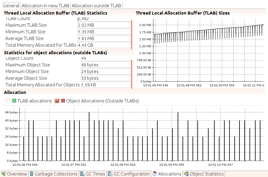
In the five seconds selected in this recording, 49 objects were allocated outside of TLABs; the maximum size of those objects was 48 bytes. Since the minimum TLAB size is 1.35 MB, we know that these objects were allocated on the heap only because the TLAB was full at the time of allocation—they were not allocated directly in the heap because of their size. That is typical immediately before a young GC occurs (as eden—and hence the TLABs carved out of eden—becomes full).
The total allocation in this period is 1.59 KB; neither the number of allocations nor the size in this example are a cause for concern. There will always be some object allocated outside of TLABs, particularly as eden approaches a young collection. Compare that example to Figure 6-10, which shows a great deal of allocation occurring outside of the TLABs.
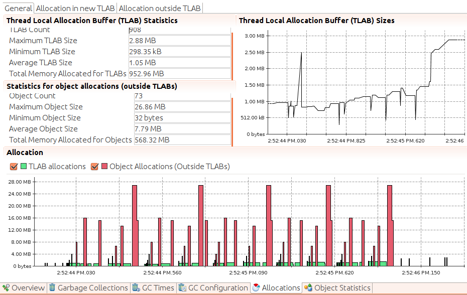
The total memory allocated inside TLABs during this recording is 952.96 MB, and the total memory allocated of objects outside of TLABs is 568.32 MB. This is a case where either changing the application to use smaller objects, or tuning the JVM to allocate those objects in larger TLABs, can have a beneficial effect. Note that there are other tabs here that can display the actual objects that were allocated out of the TLAB; we can even arrange to get the stacks from when those objects were allocated. If there is a problem with TLAB allocation, JFR will pinpoint it very quickly.
In the open-source version of the JVM (without JFR), the best thing to do
is monitor the
TLAB allocation by adding the
-XX:+PrintTLAB
flag to the command line. Then, at
every young collection, the GC log will contain two kinds of line: a line
for each thread describing the TLAB usage for that thread, and a summary line
describing the overall TLAB usage of the JVM.
The per-thread line looks like this:
TLAB: gc thread: 0x00007f3c10b8f800 [id: 18519] desired_size: 221KB
    slow allocs: 8  refill waste: 3536B alloc: 0.01613    11058KB
    refills: 73 waste  0.1% gc: 10368B slow: 2112B fast: 0B
The “gc” in this output means that the line was printed during GC; the thread
itself is a regular application thread. The size of this thread’s TLAB is
221 KB. Since the last young collection, it allocated 8 objects from the
heap (slow allocs); that was 1.6% (0.01613) of the total
amount of allocation done by this thread, and it amounted to 11,058 KB. 0.1% of
the TLAB was “wasted,” which comes from three things: 10,336 bytes were free
in the TLAB when the current GC cycle started; 2,112 bytes were free in other
(retired) TLABs, and 0 bytes were allocated via a special “fast” allocator.
After the TLAB data for each thread has been printed, the JVM provides a line of summary data:
TLAB totals: thrds: 66  refills: 3234 max: 105
        slow allocs: 406 max 14 waste:  1.1% gc: 7519856B
        max: 211464B slow: 120016B max: 4808B fast: 0B max: 0B
In this case, 66 threads performed some sort of allocation since the last young collection. Among those threads, they refilled their TLABs 3,234 times; the most any particular thread refilled its TLAB was 105. Overall there were 406 allocation to the heap (with a maximum of 14 done by one thread), and 1.1% of the TLABs were wasted from the free space in retired TLABs.
In the per-thread data, if threads show a large number of allocations outside of TLABs, consider resizing them.
Sizing TLABs
Applications that spend a lot of time allocating objects outside of TLABs will benefit from changes that can move the allocation to a TLAB. If there are only a few specific object types that are always allocated outside of a TLAB, then programmatic changes are the best solution.
Otherwise—or if programmatic changes are not possible—you can attempt to resize the TLABs to fit the application use case. Because the TLAB size is based on the size of eden, adjusting the new size parameters will automatically increase the size of the TLABs.
The size of the TLABs can be set explicitly using the flag
-XX:TLABSize=N
(the default value, 0, means to use the dynamic calculation
previously described). That flag sets only the initial size of the TLABs; to
prevent resizing at each GC, add
-XX:-ResizeTLAB
(the default for that
flag is true on most common platforms). This is the easiest (and, frankly,
the only really useful) option for exploring the performance of adjusting
the TLABs.
When a new object does not fit in the current TLAB (but would fit within a
new, empty TLAB), the JVM has a decision to make: whether
to
allocate the object in the heap, or whether to retire the current TLAB
and allocate a new one.
That decision is based on several parameters. In the TLAB logging output,
the refill waste value gives the current threshold for that decision:
if the TLAB cannot accommodate a new object that is larger than that value,
then the new object will be allocated in the heap. If the object in question
is smaller than that value, the TLAB will be retired.
That value is dynamic, but it begins by default at 1% of the TLAB size—or, specifically, at the value specified by
-XX:TLABWasteTargetPercent=N.
As each allocation is done outside the
heap, that value is increased by the value of
-XX:TLABWasteIncrement=N
(the default is 4). This prevents a thread from reaching the threshold
in the TLAB
and continually allocating objects in the heap—as the target percentage
increases, the chances of the TLAB being retired also increases. Adjusting
the
TLABWasteTargetPercent
value also adjusts the size of the TLAB, so
while it is possible to play with this value, its effect is not always
predictable.
Finally, when TLAB resizing is in effect, the minimum size of a TLAB can
be specified with
-XX:MinTLABSize=N
(the default is 2 KB). The maximum size
of a TLAB is slightly less than 1 GB (the maximum space that can be occupied
by an array of integers, rounded down for object alignment purposes), and is
not able to be changed.
Quick Summary
- Applications that allocate a lot of large objects may need to tune the TLABs (though often using smaller objects in the application is a better approach).
Humongous Objects
Objects that are allocated outside of a TLAB are still allocated within Eden when possible. If the object cannot fit within Eden, then it must be allocated directly in the old generation. That prevents the normal GC lifecycle for that object, so it is short-lived, GC is negatively affected. There’s little to do in that case other than change the application so that it doesn’t need those short-lived huge objects.
Humongous objects are treated differently in G1, however—G1 will allocate them in the old generation if they are bigger than a G1 region. So applications that use a lot of humongous objects in G1 may need special tuning to compensate for that.
G1 Region Sizes
G1 divides the heap into a number of regions, each of which has a fixed size.
The region size is not dynamic; it is determined at startup based on
the minimum size of the heap (the
value of Xms). The minimum region size is 1 MB.
If the minimum heap size is greater
than 2 GB, the size of the regions will be set according to this formula
(using log base 2):
region_size = 1 << log(Initial Heap Size / 2048);
In short: the region size is the smallest power of two such that there are close to 2048 regions when the initial heap size is divided. There are some minimum and maximum constraints in use here too; the region size is always at least 1 MB and never more than 32 MB. Table 6-3 sorts out all the possibilities.
| Heap Size | Default G1 Region Size |
Less than 4GB | 1 MB |
Between 4GB and 8GB | 2 MB |
Between 8GB and 16GB | 4 MB |
Between 16GB and 32GB | 8 MB |
Between 32GB and 64GB | 16 MB |
Larger than 64GB | 32 MB |
The size of a G1 region can be set with the
-XX:G1HeapRegionSize=N
flag
(the default for which is nominally 0, meaning to use the dynamic value
just described). The value given here should be a power of two (e.g., 1 MB
or 2 MB); otherwise it is rounded down to the nearest power of two.
Humongous Objects
If the G1 region size is 1 MB and a program allocates an array of two million bytes, the array will not fit within a single G1 region. But these humongous objects must be allocated in contiguous G1 regions. If the G1 region size is 1 MB, then to allocate a 3.1 MB array, G1 must find four contiguous regions within the old generation in which to allocate the array.[35] This defeats the way G1 normally performs compaction, which is to free arbitrary regions based on how full they are. Often, G1 will have to perform a full GC in order to find contiguous regions.
Because the humongous object is allocated directly in the old generation, it cannot be freed during a young collection. So if the object is short-lived, this also defeats the generational design of the collector. The humongous object will be collected during the concurrent G1 cycle. On the bright side, the humongous object can be freed quickly since is the only object in the regions it occupies. Humongous objects are freed during the cleanup phase of the concurrent cycle (rather than during a mixed GC).
Increasing the size of a G1 region so that all objects the program will allocate can fit within a single G1 region can make G1 more efficient.
To determine if humongous object allocation is causing the full GCs in a particular application, the GC log must have adaptive size policy logging enabled. When the application allocates a humongous object, G1 will first attempt to start a concurrent cycle:
5.349: [G1Ergonomics (Concurrent Cycles) request concurrent cycle initiation,
    reason: occupancy higher than threshold, occupancy: 483393536 bytes,
    allocation request: 524304 bytes, threshold: 483183810 bytes (45.00 %),
    source: concurrent humongous allocation]
 ...
5.350: [GC pause (young) (initial-mark) 0.349: [G1Ergonomics
    (CSet Construction) start choosing CSet, _pending_cards:
    1624, predicted base time: 19.74 ms, remaining time: 180.26 ms,
    target pause time: 200.00 ms]
This indicates that the humongous allocation occurred, triggering a concurrent G1 cycle to begin. In this entry, the allocation succeeded without other effects on GC (G1 happened to find the needed contiguous regions).
If no contiguous regions are found, G1 will run a full GC:
25.270: [G1Ergonomics (Heap Sizing) attempt heap expansion,
    reason: allocation request failed, allocation request: 48 bytes]
25.270: [G1Ergonomics (Heap Sizing) expand the heap,
    requested expansion amount: 1048576 bytes,
    attempted expansion amount: 1048576 bytes]
25.270: [G1Ergonomics (Heap Sizing) did not expand the heap,
    reason: heap expansion operation failed]
25.270: [Full GC 1535M->1521M(3072M), 1.0358230 secs]
      [Eden: 0.0B(153.0M)->0.0B(153.0M)
       Survivors: 0.0B->0.0B Heap: 1535.9M(3072.0M)->1521.3M(3072.0M)]
      [Times: user=5.24 sys=0.00, real=1.04 secs]
Because the heap could not be expanded to accommodate the new humongous
object, G1 had to perform a full GC to compact the heap in order to
provide the contiguous regions needed to fulfill the request, Without the
additional logging provided by enabling
PrintAdaptiveSizePolicy,
the standard G1 GC log does not provide enough information to diagnose
this situation.
To prevent this full GC, first determine the size of the humongous objects that are causing the issue (that value is in the log above: 524,304 bytes in this example). A better next step is to reduce the size of those objects rather than tune the JVM around them. If that is not possible, calculate the region size that will be needed to accommodate those objects. G1 considers an object to be humongous if it will fill more than 50% of a region. Hence, if the object in question is 524,304 bytes, the G1 region size needs to be at least 1.1MB. Since G1 regions are always a power of two, the G1 region size must be set to 2 MB in order for those objects to be allocated in a standard G1 regions.
Quick Summary
- G1 Regions are sized in powers of two, starting at 1 MB.
- Heaps that have a very different maximum size than initial size will have too many G1 regions; the G1 region size should be increased in that case.
- Applications that allocate objects that are larger than half the size of a G1 region should increase the G1 region size so that the objects can fit within a G1 region. An application must allocate an object that is at least 512 KB for this to apply (since the smallest G1 region is 1 MB).
AggressiveHeap
The
AggressiveHeap
flag (by default, false), was introduced in an early version of Java as an attempt to make it easier to easily set a variety of command-line arguments—arguments that would be appropriate for a very large machine with a lot of memory which is running a single JVM. It applies only to 64-bit JVMs.
Although the flag has been carried forward since those versions and is still present, it is no longer recommended (though it is not yet officially deprecated). The problem with this flag is that it hides the actual tunings that it adopts, making it quite hard to figure out what the JVM is actually setting. Some of the values it sets are now set ergonomically based on better information about the machine running the JVM, so that there are actually cases where enabling this flag hurts performance. I have often seen command lines that include this flag and then later override values that it sets.[36]
For the record, Table 6-4 lists all the tunings that are automatically set when the
AggressiveHeap
flag is enabled.
| Flag | Value |
Xmx | The minimum of half of all memory, or all memory - 160M |
Xms | The same as Xmx |
NewSize | 3/8ths of whatever was set as |
UseLargePages | true |
ResizeTLAB | false |
TLABSize | 256K |
UseParallelGC | true |
ParallelGCThreads | Same as current default |
YoungPLABSize | 256K (default is 4K) |
OldPLABSize | 8K (default is 1K) |
CompilationPolicyChoice | 0 (which is the current default) |
ThresholdTolerance | 100 (default is 10) |
ScavengeBeforeFullGC | false (default is true) |
BindGCTaskThreadsToCPUs | true (default is false) |
Those last six flags are obscure enough that I have not discussed them elsewhere in this book. Briefly, they cover these areas:
- PLAB sizing: PLABs are promotion local allocation buffers—these are per-thread regions used during scavenging the generations during a GC. Each thread can promote into a specific PLAB, negating the need for synchronization (analogous to the way TLABs work).
- Compilation Policies: The JVM ships with some alternate JIT compilation algorithms, The current default algorithm was, at one time, somewhat experimental, but this is now the recommended policy.
-
Disabling Young GCs before Full GCs: setting
ScavengeBeforeFullGCto false means that when a full GC occurs, the JVM will not perform a young GC before a full GC. That is usually a bad thing, since it means that garbage objects in the young generation (which are eligible for collection) can prevent objects in the old generation from being collected. Clearly there is (or was) a point in time where that setting made sense (at least for certain benchmarks), but the general recommendation is not to change that flag. - Binding GC threads to CPUS: setting the last flag in that list means that each parallel GC thread is bound to a particular CPU (using OS-specific calls). In limited circumstances—when the GC threads are the only thing running on the machine, and heaps are very large—that makes sense. In the general case, it is better if GC threads can run on any available CPU.
As with all tunings, your mileage may vary, and if you carefully test the
AggressiveHeap
flag and find that it improves performance, then by all means use it. Just be aware of what it is doing behind the scenes, and realize that whenever the JVM is upgraded, the relative benefit of this flag will need to be re-evaluated.
Quick Summary
-
The
AggressiveHeapflag is a legacy attempt to set a number of heap parameters to values that make sense for a single JVM running on a very large machine. - Values set by this flag are not adjusted as JVM technology improves, so its usefulness in the long run is dubious (even though it still is often used).
Full Control over Heap Size
Sizing the Heap discussed the default values for the initial minimum and maximum size of the heap. Those values are dependent on the amount of memory on the machine as well as the JVM in use, and the data presented there had a number of corner cases to it. If you’re curious about the full details about how the default heap size is actually calculated, this section will explain the details. Those details include some very low-level tuning flags; in certain circumstances, it might be more convenient to adjust the way those calculations are done (rather than simply setting the heap size). This might be the case if, for example, you want to run multiple JVMs with a common (but adjusted) set of ergonomic heap sizes. For the most part, the real goal of this section is to complete the explanation of how those default values are chosen.
The default sizes are based on the amount of memory on a machine, which is
can be set with the
-XX:MaxRAM=N
flag. Normally, that value is calculated by the JVM by inspecting the
amount of memory on the machine.
However, the JVM limits
MaxRAM
to 1 GB for the client
compiler, 4 GB for 32-bit server compilers, and 128 GB for 64-bit compilers.
The maximum heap size is 1/4 of
MaxRAM.
This is why the
default heap size can vary: if the physical
memory on a machine is less than
MaxRAM,
the default heap size is
1/4 of that. But even if hundreds of GB of RAM are available, the most the JVM
will use by default is 32 GB: 1/4 of 128 GB.
The default maximum heap calculation is actually this:
Default Xmx = MaxRAM / MaxRAMFraction
Hence,
the default maximum heap can also be set by adjusting the value of the
-XX:MaxRAMFraction=N
flag, which defaults to 4.
Finally, just to
keep things interesting, the
-XX:ErgoHeapSizeLimit=N
flag can also be set
to a
maximum default value that the JVM should use. That value is 0 by default
(meaning to ignore it); otherwise, that limit is used if it is smaller than
MaxRAM / MaxRAMFraction.
On the other hand, on a machine with a very small amount of
physical memory, the JVM wants to be sure it leaves enough memory for the
operating system. This is why the JVM will limit the maximum
heap to 96MB or less on machines with only 192MB of memory. That
calculation is based on the value of the
-XX:MinRAMFraction=N
flag, which defaults to 2:
if ((96 MB * MinRAMFraction) > Physical Memory) {
    Default Xmx = Physical Memory / MinRAMFraction;
}
The initial heap size choice is similar, though it has fewer complications. The initial heap size value is determined like this:
Default Xms = MaxRAM / InitialRAMFraction
As can be concluded from the default minimum heap sizes,
the default value of
the
InitialRAMFraction
flag is 64. The one caveat here occurs if that value is less than 5 MB—or,
strictly speaking, less than the values specified by
-XX:OldSize=N
(which defaults to 4 MB) plus
-XX:NewSize=N
(which defaults to 1 MB).
In that case, the sum of the old and new size is used as
the initial heap size.
Quick Summary
- The calculations for the default initial and maximum heap sizes are fairly straightforward on most machines.
- Around the edges, these calculations can be quite involved.
Summary
The past two chapters have spent a lot of time delving into the deep details of how GC (and its various algorithms) work. If garbage collection is taking longer than you’d like, knowing how all of that works should aid you in taking the necessary steps to improve things.
Now that we understand all the details, let’s take a step back and look at to determine an approach to choosing and tuning a garbage collector. Here’s a quick set of questions to ask yourself to help put everything in context.
- Can your application tolerate some full GC pauses?
- If so, then the throughput collector will likely offer the best performance, while using less CPU and a smaller heap than other collectors. If not, then choose a concurrent collector—for smaller heaps, either CMS or G1. For larger heaps, G1.
- Are you getting the performance you need with the default settings?
Try the default settings first. As GC technology matures, the ergonomic (automatic) tuning gets better all the time.
If you’re not getting the performance you need, make sure that GC is your problem. Look at the GC logs and see how much time you’re spending in GC and how frequently the long pauses are. For a busy application, if you’re spending 3% or less time in GC, you’re not going to get a lot out of tuning (though you can always try and reduce outliers if that is your goal).
- Are the pause times you have somewhat close to your goal?
- If they are, then adjusting the maximum pause time may be all you need. If they aren’t, then you need do do something else. If the pause times are too large but your throughput is okay, you can reduce the size of the young generation (and for full GC pauses, the old generation); you’ll get more, but shorter pauses.
- Is throughput lagging even though GC pause times are short?
You need to increase the size of the heap (or at least the young generation).
More isn’t always better—bigger heaps lead to longer pause times. Even with a concurrent collector, a bigger heap means a bigger young generation by default, so you’ll see longer pause times for young collections. But if you can, increase the heap size, or at least the relative sizes of the generations.
- Are you using a concurrent collector and seeing full GCs due to concurrent mode failures?
- If you have available CPU, try increasing the number of concurrent GC threads or starting the background sweep sooner by adjusting the initiating occupancy fraction. For G1, the concurrent cycle won’t start if there are pending mixed GCs; try reducing the mixed GC count target.
- Are you using a concurrent collector and seeing full GCs due to promotion failures?
- In CMS, a promotion failure indicates that the heap is fragmented. There is little to do about that; using a larger heap and/or performing the background sweep sooner can help in some cases. It may be better to try G1 instead. In G1, an evacuation failure (to-space overflow) indicates essentially the same thing, but the fragmentation can be solved if G1 performs its background sweeping sooner and mixed GCs faster. Try increasing the number of concurrent G1 threads, adjusting the initiating heap occupancy, or reducing the mixed GC count target.
[27] Actually, 227893 KB is only 222 MB. For ease of discussion, I’ll just truncate the KBs by 1000 in this chapter. Pretend I am a disk manufacturer.
[28] If permgen runs out of room, the JVM will run a full GC to collect pergmen, and you will see the size of permgen change—which is the only way to detect if permgen has been collected. Also, this example is from Java 7; the Java 8 output will include similar information on the metaspace.
[29] Although the default
value for that flag is 70, this example started the CMS threads when the old
generation was 50% full because the UseCMSInitiatingOccupancyOnly flag
was not set.
[30] Fortunately, there were spare CPU cycles on the machine for the parallel G1 threads, or the pause would have been longer.
[31] If this occurs frequently, it is an indication that G1 needs to be better tuned, as discussed in the next section.
[32] It is likely
this value will become a tunable parameter at some point; the experimental
name for the parameter (available in experiment builds of the open source
code) is
-XX:G1MixedGCLiveThresholdPercent=N.
[33] The survivor spaces are also referred to as the “to” and “from” space; during each collection, objects are moved out of the “from” space into the “to” space. “from” and “to” are simply pointers that switch between the two survivor spaces on every collection.
[35] The rest of the last region will remain empty, wasting .9 MB of space.
[36] For the record, that works: later values in the command line currently override earlier values. That behavior is not guaranteed.