CHAPTER 11: Supervised Machine Learning

Supervised machine learning is truly the core of data science, as all of the directly applicable insights stem from the outputs of this part of the process. Its most common types are classification and regression, depending on the nature of the target variable.

It would be quite a feat to do this topic justice, as there are so many different methods that fall under its umbrella. However, we’ll cover the most commonly used ones and demonstrate how they can be implemented in Julia, relying on the following packages: DecisionTree, BackpropNeuralNet, ELM and GLM. Make sure that you have them installed on your computer before going through the examples in this chapter.

In this chapter we will examine the following topics:

• • Rationale and overview of supervised learning
• • Decision trees (classification)
• • Regression trees
• • Random forests
• • Basic neural networks (ANNs)
• • Extreme Learning Machines (ELMs)
• • Statistical models for regression
• • Other supervised learning methods.

We’ll be working with both the Magic and the OnlineNewsPopularity datasets, so make sure that you have loaded these into memory, too. We’ll also use a couple of auxiliary functions for some essential data engineering, so make sure that you load the files sample.jl and normalize.jl into memory. Finally, make sure that you load a few other auxiliary functions, such as MSE(), located in the first part of this chapter’s notebook file.

Supervised learning involves getting the computer to create a generalization based on some labeled data, and then use that generalization to predict the labels of a set of unlabeled data. There are several ways of doing this, each one representing a particular supervised learning method. Although there are two main methodologies of supervised learning, classification and regression, it is sometimes the case that a supervised learning system does both.

The goal of this type of machine learning is to be able to make accurate and reliable predictions. We could learn the labels of an unlabeled dataset via unsupervised learning, but this would be limited to more obvious structural patterns in the dataset. If we have some additional information in the form of labels, then we can harness these invaluable assets only through specialized methods: the supervised learning algorithms.

Although many people use logistic models (e.g. logistic regression) for this purpose, we will veer away from those. Logistic models are by far the weakest methods out there; apart from easy interpretability, they don’t have any other real advantages. If you’re interested in logistic models, you can easily implement them yourself.

Modern machine learning started when data analysts wanted to go beyond what logistic models could offer. In the rest of the chapter we’ll focus on more interesting methods, examining their role in data science as well as how they are implemented in Julia. However, we won’t be looking much at the use of ensembles (combinations of supervised learning systems), as this is a more sophisticated approach that requires substantial machine learning expertise.

Decision Trees

A decision tree is basically a series of rules that is applied to the dataset, eventually leading to a choice between two or more classes. It is like playing the “20 questions” game, but with a limited set of objects that you are trying to guess, and without a strict number of questions that can be asked.

Mathematically, decision trees are graphs (we’ll talk more about graphs in the next chapter) that are designed to examine a limited number of possibilities, in order to arrive at a reliable conclusion about what class each data point is in. These possibilities are modeled as nodes and edges, as you can see in the example in Figure 11.1. In this figure, different fruits are classified based on their color, shape, size and taste. Not all of these characteristics are used for each classification; the ones that are used depend on the output of each test (node).

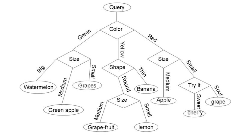
Figure 11.1 An example of a typical decision tree. Used with permission from www.projectrhea.com.

Decision trees are great for cases where the features are rich in information, more or less independent from each other, and not too large. They are excellent for interpretability and easy to build and use. Also, due to their nature, they don’t require any normalization in the data they use.

Implementing decision trees in Julia

You can implement decision trees in Julia by making use of the DecisionTree package as follows:

In[1]: using DecisionTree

Next, we’ll need to define some parameters for the decision trees we use. The first one is the combined purity parameter, which refers to the proportion of correct labels in a leaf node. Although it’s tempting to make this equal to 1.0, it’s unwise because overfitting will unmistakably result. A very low value would not work, either. Usually a value of 0.9 works well for the majority of applications.

In[2]: CP = 0.9

Since we’ll be doing some cross-validation as well, we’ll need to define the corresponding parameter for it.

In[3]: K = 5

Before we move on, let’s define a couple more parameters, namely the tree depth (td) and the number of leaves to be used for averaging in regression applications (nl). The tree depth is mainly for viewing purposes, and applies to a single decision tree. Even though it is not absolutely necessary, it can be useful in understanding and interpreting the decision tree we build. Some good values for these parameters are the following (feel free to experiment with other ones if you want):

In[4]: td = 3

    nl = 5

Now, let’s see how the decision trees are built and used to classify the magic dataset. First, let’s build a tree and tidy it up using the build_tree() and prune_tree() functions respectively:

In[5]: model = build_tree(T1, P1)

    model = prune_tree(model, CP)

The “pruning” of the tree is not truly essential, but it is useful as it keeps the tree simple and therefore less prone to overfitting. The output of all this is the following:

Out[5]: Decision Tree

    Leaves: 1497

    Depth: 30

Believe it or not, this is a relatively small decision tree, especially considering that we are using the dataset as-is. Naturally, if we were to perform some dimensionality reduction, the resulting tree would be even smaller. The above command is not guaranteed to produce the exact same tree on your computer, due to the stochastic nature of the decision tree. Let’s now see what this bonsai of ours looks like:

In[6]: print_tree(model, td)

Feature 9, Threshold -0.3096661121768262

L-> Feature 1, Threshold 1.525274809976256

  L-> Feature 9, Threshold -0.6886748399536539

    L->

    R->

  R-> Feature 7, Threshold -2.3666522650618234

    L-> h : 99/99

    R->

R-> Feature 1, Threshold -0.16381866376775667

  L-> Feature 3, Threshold -1.0455318957511963

    L->

    R->

  R-> Feature 1, Threshold 0.42987863636363327

    L->

    R->

From this short preview of the built tree, it becomes clear that feature 1 (fLength) plays an important role in distinguishing between the two classes of radiation observed by the telescope. This is because it appears on the first leaf and because it appears more than once. We can also note the thresholds used in all the leaves shown here, to better understand the feature. Perhaps we’ll eventually want to make this feature discreet. If that’s the case, the thresholds used here could be a good starting point. Now let’s see how all this can be used to make some predictions, using the apply_tree() function:

In[7]: pred = apply_tree(model, PT1)

Out[7]: 1902-element Array{Any,1}:

    “g”

    “g”

    “g”

    “g”

    “g”

This will yield an array populated by the predicted labels for the test set. The type of the output as well as the values themselves will be the same as the original targets, i.e. “g” and “h” for each one of the two classes. What about the certainty of the classifier, though? This can be made available through the apply_tree_proba() function, as long as we provide the list of class names (Q):

In[8]: prob = apply_tree_proba(model, PT1, Q)

Out[8]: 1902x2 Array{Float64,2}:

    1.0  0.0  

    1.0  0.0  

    1.0  0.0  

    1.0  0.0  

    0.985294  0.0147059

Each one of the columns of the output corresponds to the probability of each class. This is similar to the output of a neural network, as we’ll see later on. Actually, the decision tree calculates these probabilities first and then chooses the class based on the probabilities.

As all this may not be enough to assess the value of our classification bonsai, we may want to apply some KFCV to it. Fortunately, the DecisionTree package makes this much easier as it includes a cross validation function, nfoldCV_tree():

In[9]: validation = nfoldCV_tree(T_magic, F_magic, CP, K)

The result (which is too long to be included here) is a series of tests (K in total), where the confusion matrix as well as the accuracy and another metric are shown. Afterwards, a summary of all the accuracy values is displayed, to give you a taste of the overall performance of the decision trees. Here is a sample of all this, from the final cross validation round:

2x2 Array{Int64,2}:

2138 327

368 971

Fold 5

Classes: Any[“g”,”h”]

Matrix:  

Accuracy: 0.8172975814931651

Kappa:  0.5966837444531773

This may not satisfy the most demanding data scientists out there–those who rely on more insightful metrics, like the ones we described in Chapter 9, where performance metrics are discussed. Generally, though, the confusion matrix will prove valuable when calculating the metrics we need, so we don’t have to rely on the accuracy provided by the cross validation function of this package.

Decision tree tips

Although decision trees are great for many problems, they have some issues that you ought to keep in mind. For example, they don’t deal well with patterns that are not in the form of a rectangle in the feature space. These patterns produce a large number of rules (nodes), making them cumbersome and hard to interpret. Also, if the number of features is very large, they take a while to build, making them impractical. Finally, due to their stochastic nature, it is difficult to draw conclusions about which features are more useful by just looking at them.

Overall, decision trees are decent classification systems and are worth a try, particularly in cases where the dataset is relatively clean. They can be ideal as a baseline, while they can work well in an ensemble setting as we’ll see later on in the Random Forests section.

Regression Trees

The regression tree is the counterpart of the decision tree, applicable in regression problem-solving settings. Instead of labels, they predict values of a continuous variable. The function of regression trees relies on the fact that decision trees can predict probabilities (of a data point belonging to a particular class). These probabilities are by nature continuous, so it is not a stretch to transform them into another continuous variable that approximates the target variable of a regression problem. So, the mechanics underneath the hood of the regression trees are the same as those of the decision trees we saw previously. Let’s now look at how all this is implemented in Julia, via the DecisionTree package.

Implementing regression trees in Julia

We can build and use a regression tree in Julia using the same functions as in the decision tree case. The only difference is that when building a regression tree, we need to make use of the number of leaves parameter (nl) when applying the build_tree() function. This basically tells Julia to treat the target as a continuous variable, and approximate it by taking the average of the number of leaves. So, if we were to train a regression tree model in this fashion we would type:

In[10]: model = build_tree(T2, P2, nl)

Like before, we would get something like this as an output:

Out[10]: Decision Tree

  Leaves: 14828

  Depth: 19

Although this is a decision tree object as far as Julia is concerned, its application lies in regression. So, if we were to apply it on our data, here is what would happen:

In[11]:  pred = apply_tree(model, PT2)

Out[11]: 1902-element Array{Float64,1}:

  1500.0

  5700.0

  5200.0

  1800.0

  426.0

This output would go on for a while, with all of the elements of the output array being floats, just like the targets we trained the model with (T2). Let’s see how well these predictions approximate the actual values (TT2):

In[12]:  MSE(pred, TT2)

Out[12]: 2.2513992955941114e8

This is not bad at all, considering how varied the target variable is. Naturally, this can be improved by tweaking the regression tree a bit. However, for now we’ll focus on other, more powerful supervised learning systems.

Regression tree tips

As you might expect, regression trees have the same limitations as their classification counterparts. So although they can be great as baselines, you will rarely see them in production. Nevertheless, it is important to learn how to use them, as they are the basis of the next supervised learning system we’ll examine in this chapter.

Random Forests

As the name eloquently suggests, a random forest is a set of decision or regression tree systems working together. This is by far the most popular ensemble system used by many data scientists, and the go-to option for the majority of problems. The main advantage of random forests is that they generally avoid overfitting and always outperform a single tree-based system, making them a more comprehensive alternative. Configuring them, however, can be a bit of a challenge. The optimum parameter settings (number of random features, number of trees, and portion of samples used in every tree) depends on the dataset at hand.

Random forests are modestly interpretable, but they lack the ease of use and interpretability of single-tree systems. Random forests tend to obtain better generalizations, making them suitable for challenging problems, too. As a bonus, mining the trees in a random forest can yield useful insights about which features perform better, as well as which ones work well together. Also, they are generally fast, though their performance heavily depends on the parameters used.

Implementing random forests in Julia for classification

You can implement random forest using the following Julia code and the DecisionTree package. First, let’s get some parameters set: the number of random features in each training session (nrf), the number of trees in the forest (nt), and the proportion of samples in every tree (ps):

In[13]: nrf = 2

    nt = 10

    ps = 0.5

Next, we can build the forest based on the data of the magic dataset, using the build_forest() function and the above parameters:

In[14]:  model = build_forest(T1, P1, nrf, nt, ps)

Out[14]: Ensemble of Decision Trees

  Trees:   10

  Avg Leaves: 1054.6

  Avg Depth: 31.3

Contrary to what you might expect, the forest has significantly fewer leaves on each of its trees, but many more branches (expressed as depth). This is because of the parameters we chose, and for a good reason. If we were to use all the features on each tree and all of the data points, we would end up with a bunch of trees that would be similar to each other. Although such a forest could be better than any individual tree, it wouldn’t be as good as a forest with more diversity in its members.

This diversity lies not just in the structure of the trees, but also in the rules that each one encompasses. Just like in nature, a diverse forest with a large variety of members tends to flourish in terms of performance. In this case, our mini-forest of ten diverse trees is far more robust than any tree we could build individually, in the same number of attempts.

It is not expected that you’ll blindly believe this (we are all scientists, after all). Instead, let’s test this claim out by making use of this classification forest, using the apply_forest() function as follows:

In[15]: pred = apply_forest(model, PT1)

The prediction output would be similar to that of a single decision tree, which is why we omit it here.

Just like in the decision tree case, we can also calculate the corresponding probabilities of the above classification, this time using the apply_forest_proba() function:

In[16]: prob = apply_forest_proba(model, PT1, Q)

Here is what these probabilities would look like in the case of the random forest:

Out[16]: 1902x2 Array{Float64,2}:

  1.0 0.0

  0.5 0.5

  0.9 0.1

  0.6 0.4

  0.9 0.1

Note how the probabilities are far more discreet than the ones in the single decision tree. That’s because they are based on the outputs of the individual trees that make up the forest; since they are ten in total, the probabilities would be in the form x / 10, where x = 0, 1, 2, ..., 10.

Let’s see how the forest performs overall now. To do that, we’ll use the corresponding cross validation function, nforldCV_forest():

In[17]: validation = nfoldCV_forest(T_magic, F_magic, nrf, nt, K, ps)

Like in the decision tree case, this function provides a long output, including this sample:

2x2 Array{Int64,2}:

2326 118

408 952

Fold 5

Classes: Any[“g”,”h”]

Matrix:  

Accuracy: 0.8617245005257623

Kappa:  0.6840671243518406

Mean Accuracy: 0.8634069400630915

We don’t need to look at everything to see how this result is much better than that of a single decision tree. Of course, the difference is much greater if the baseline is lower. Whatever the case, a random forest is bound to perform much better, at least in terms of overall performance as measured by the accuracy metric.

Implementing random forests in Julia for regression

Let’s look at how random forests can be applied in a regression setting, ultimately outperforming a single regression tree. Since we’ll be using the same parameters as in the previous examples, we can just go straight into the building of the regression random forest. Use the build_forest() function, but this time with the number of leaves parameter (nl) also added to the mix:

In[18]:  model = build_forest(T2, P2, nrf, nt, nl, ps)

Out[18]: Ensemble of Decision Trees

  Trees:   10

  Avg Leaves: 2759.9

  Avg Depth: 34.3

This time we get a set of denser trees (more leaves), that are also slightly longer (more depth). This change is to be expected, since a regression tree is generally richer in terms of nodes in order to provide accurate approximations of the target variable, which is also more complex than that of a classification task.

Let’s now see how all this plays out in the predictions space. Like before, we’ll use the apply_forest() function:

In[19]: pred = apply_forest(model, PT2)

Finally, let’s take a look at how this forest of regression trees performs overall by applying KFCV. We’ll use the nfoldCV_forest() function like before, but with the number of leaves parameter (nl) added in its inputs:

In[20]: validation = nfoldCV_forest(T_ONP, F_ONP, nrf, nt, K, nl, ps)

Here is part of the output:

Fold 5

Mean Squared Error:   1.5630249391345486e8

Correlation Coeff:   0.14672119043349965

Coeff of Determination: 0.005953472140385885

If we were to take the average of all the mean squared errors of the five tests, we would end up with a figure close to 1.40e8. This is much smaller than the MSE of the single regression tree we saw previously (about 2.25e8), as we would expect.

Random forest tips

Despite their popularity, random forests are not the best supervised learning systems out there. They require a lot of data in order to work well, and the features need to be uncorrelated to some extent. Also, it is virtually impossible to tweak them so that they work well for heavily unbalanced datasets, without altering the data itself.

An advantage of random forests is that if we examine them closely, we can glean some useful insight about the value of each feature. This is made possible by the frequency of each feature being used in a leaf node. Unfortunately the current implementation of random forests in the DecisionTree package doesn’t allow this.

Overall, decision forests are good for baseline measures, and are fairly easy to use. Additionally, the DecisionTree package is powerful and well-documented, so it is definitely easy to explore this kind of supervised learning systems further.

Basic Neural Networks

Even up until fairly recently, this was an esoteric part of machine learning that few people cared about and even fewer understood. Despite this, neural networks are by far the most influential and the most robust alternative to statistical learning. Fancy math aside, neural networks are abstraction models that emulate processes of the human brain by using a hierarchical structure of mathematical processes.

Instead of biological cells, neural networks have mathematical ones, which share the same name as their counterparts: neurons. Instead of transmitting electrical signal through neurotransmitters, they use float variables. Finally, instead of an excitation threshold corresponding to a cell’s choice of whether to propagate the signal it receives, they have a mathematical threshold and a series of coefficients called weights. Overall, they are a functional abstraction of the physiological neural tissues, and they do a good job processing information in a similar manner. In Figure 11.2 you can see a typical artificial neural network (ANN).

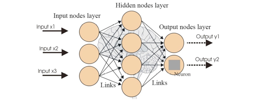
Figure 11.2. A typical artificial neural network (ANN).

ANNs are basically graphs that perform classification and regression, like tree-based systems, but employ a series of more sophisticated algorithms. A neural network is a graph that can both represent the dataset it is trained on, while simultaneously using this information for predictions. Structurally, ANNs have their neurons organized in layers; the basic ANNs have three to four layers, one or two of which are hidden. These hidden layers represent the meta-features that a neural network builds and uses for its predictions.

We encourage you to learn more about ANNs, paying close attention to how they are trained and the overfitting issues that may arise. And although it’s generally a good idea to read the documentation of Julia packages, in this case it would be best if you didn’t, since the example in the BackpropNeuralNet package may lead you to the wrong conclusions about how ANNs work.

Implementing neural networks in Julia

Let’s see now how we can get a basic ANN working using the BackpropNeuralNet package on the magic dataset. First, we need to prepare the data, particularly the target variable, since an ANN only works with numeric data (the ones in this package work with just floats). In order to get the ANN to understand the target variable we need to transform it into a n x q matrix, where n is the number of data points in either the training or the testing set, and q the number of classes. Each row must have 1.0 at the column of the corresponding class. We have coded this transformation into a simple function called vector2ANN (see the first part of the notebook).

For now we need to define some parameters for the ANN, namely the number of nodes in each layer and the number of iterations for the training (usually referred to as epochs):

In[21]: nin = size(F_magic,2) # number of input nodes

    nhln = 2*nin # number hidden layer nodes

    non = length(Q) # number of output nodes

    ne = 1000 # number of epochs for training

Some constants for the dataset will also come in handy:

In[22]: N = length(T1)

    n = size(PT1,1)

    noc = length(Q) # number of classes

Now we can transform the target variable using the vector2ANN() function, for the training set:

In[23]: T3 = vector2ANN(T1, Q)

Finally, we are ready to work with the ANN itself. Let’s start by loading the package into memory:

In[24]: using BackpropNeuralNet

Next, we need to initialize an ANN based on the parameters we defined previously, using the init_network() function. The initial form of the ANN is a bunch of random numbers representing the various connections among its nodes. This provides us zero information up front, and may even be confusing for some people. For this reason we repress the output of this command by adding a semicolon at the end:

In[25]: net = init_network([nin, nhln, non]);

Now comes the more time-consuming part: training the neural net. Unfortunately, the package provides just the most fundamental function (train()), without any explanation of how to use it. Running it once is fast, but in order for the neural network to be trained properly, we need to apply it several times, over all the data points of the training set (curiously, the function works only with a single data point). So, here is the code we need to run to get the training of the ANN going:

In[26]: for j = 1:ne

   if mod(j,20) == 0; println(j); end #1

  

   for i = 1:N

     a = P1[i,:]

     b = T3[i,:]

     train(net, a[:], b[:])

   end

    end

If the total number of iterations (ne) is large enough, there is a chance for the ANN to train properly. However, this can be an unsettling process since we don’t know whether the training is working or whether it has crushed the Julia kernel. In order to get some kind of update, we insert the statement in #1 that basically provides us with the iteration number every 20 iterations. If we find that the ANN hasn’t been trained properly, we can run this loop again, since every time the train() function is executed, it works on the existing state of the ANN, rather than the initial one.

Once we are done with the training, we can test the performance of the ANN using the following commands:

In[27]: T4 = Array(Float64, n, noc)

    for i = 1:n

   T4[i,:] = net_eval(net, PT1[i,:][:])

    end

The above loop records the output of the neural network for each data point in the testing set. However, the format of this output is a matrix, similar to the one we used for the target variable when we trained it. To turn it into a vector we need to apply ANN2vector(), an auxiliary function we have developed for this purpose:

In[28]: pred, prob = ANN2vector(T4, Q)

This function provides the predictions, a vector similar to the original class variable, along with a probabilities vector as a bonus. The probabilities vector shows the corresponding probability for each prediction. We can now evaluate the performance of the ANN using the accuracy metric:

In[29]: sum(pred .== TT1) / n

Clearly this performance leaves a lot to be desired. This is probably due to either insufficient training, suboptimal parameters, or a combination of these. Ideally, we would train the ANN until the error on the training set falls below a given threshold, but this approach requires a more in-depth view of the topic that is well beyond the scope of this book.

Neural network tips

Many data scientists are polarized on this topic, and it has attracted a lot of attention in the past few years. The intention here is not to discredit this technology but to pinpoint its limitations. Even though it is probably one of the best systems in your toolbox, it does have some problems that make it less than ideal for certain data science applications. With this in mind, let’s look into ANNs in more depth.

First of all, they have a tendency to overfit, particularly if you don’t know how to pick the right parameters. So if you are new to them, don’t expect too much, in order to avoid disappointment. If you do spend enough time with them, however, they can work wonders and quickly become the only supervised learning systems you use. Whatever the case, be prepared to spend some time with them if you want to achieve noteworthy performance for your classification or regression task.

ANNs tend to be slow to train, particularly if you have a lot of data. So, they are better suited for large systems (ideally computer clusters). If you want to train one on your laptop, be prepared to leave it on for the rest of the afternoon, or night, or even weekend, depending on the dataset at hand.

In order to achieve particularly good generalization from an ANN, you’ll need a lot of data. This is partly to avoid overfitting, and partly because in order for the ANN to pick up the signal in your dataset, it must notice it several times, which happens best when you have a large number of data points. Alternatively, you can oversample the least represented patterns, but you have to know what you are doing, otherwise you might decrease the overall performance of the classification or regression task.

Overall ANNs are great, particularly when carefully configured. However, you may need to do some work to make them perform well. For example, you can put a series of ANNs together in an ensemble and be guaranteed a good performance. You’ll need to have resources to spare, though, as most ANNs in data science are computationally expensive, with ensembles of them even more so. Therefore, it’s best to save them for the challenging problems, where conventional supervised learning systems yield mediocre performance.

Extreme Learning Machines

The use of Extreme Learning Machines, or ELMs for short, is a relatively new network-based method of supervised learning, aiming to make the use of ANNs easier and their performance better. Although they have been heavily criticized by academics due to their similarity to another technology (randomized neural networks), this does not detract from their value.

ELMs work well and are one of the best alternatives to ANNs and other supervised learning methods. In fact, the creators of this technology claim that its performance is comparable to that of state-of-the-art deep learning networks, without their computational overhead.

Essentially, ELMs are tweaked versions of conventional ANNs with the main difference being the way they are trained. In fact, ELMs have reduced the training phase into an extremely nimble optimization task (which is probably where they get their controversial name), giving them a solid advantage over all other network-based methods.

This is achieved by first creating a series of random combinations of features, which are represented by one or more layers of nodes (the hidden layers of the ELM). Then, an optimal combo of these meta-features is calculated so as to minimize the error in the output node. All the training of the ELM lies in the connections between the last hidden layer and the output layer. This is why two separately trained ELMs on the same data may have significant differences in their weights, matrices, and even their performance. This doesn’t seem to bother many people, though, since the speed of ELMs makes it easy to try multiple iterations of the same ELM on the same data before the final model is picked.

You can learn more about this intriguing technology at the creators’ website: http://bit.ly/29BirZM, as well as through the corresponding research papers referenced there.

Implementing ELMs in Julia

The implementation of Extreme Learning Machines in Julia is made easy through the use of the ELM package (http://bit.ly/29oZZ4u), one of the best ML packages ever created in this language. Its unprecedented simplicity and ease of use is only surpassed by its excellent documentation and cleanness of code. Also, for those of you interested in researching the topic, the author of the package has even included a reference to a key article on the field. So, let’s get started by formatting the target variable in a way that is compatible with the ELMs:

In[30]: T5 = ones(N)

    T6 = ones(n)

In[31]: ind_h = (T1 .== “h”)

In[32]: T5[ind_h] = 2.0

In[33]: ind_h = (TT1 .== “h”)

In[34]: T6[ind_h] = 2.0

With the above code, we have turned the target variable into a float having values 1.0 and 2.0 for the two classes, respectively. Naturally, the numbers themselves don’t have particular significance. As long as you represent the classes with floats, the ELM will be fine with them.

Now we can proceed with loading the ELM package into memory through the familiar code:

In[35]: using ELM

Next, we need to initialize an ELM by using the ExtremeLearningMachine() function. The only parameter we need is the number of nodes in the hidden layer, which in this case is 50. This number can be any positive integer, though it usually is larger than the number of features in the dataset.

In[36]: elm = ExtremeLearningMachine(50);

Finally the time has come to train the ELM using the features and the modified target variable. We can do this using the fit() function. However, since a function with the same name exists in another package, we need to specify to Julia which one we want, by putting the package name in front of it:

In[37]: ELM.fit!(elm, P1, T5)

Unlike an ANN, an ELM will train in a matter of seconds (in this case milliseconds), so there is no need to insert a progress reporting statement anywhere. Once our system is trained, we can get a prediction going by using the predict() function on the test data:

In[38]: pred = round(ELM.predict(elm, PT1))

Note that we have applied the round() function as well. This leads to a threshold of 1.5 for the class decision (anything over 1.5 gets rounded up to 2.0 and anything below 1.5 becomes 1.0), which is an arbitrary choice for a threshold, even if it is the most intuitive one. However, it is a good starting point, as we can always change the threshold when we refine the model.

The predict() function will yield the predictions of the ELM, which will be floats around the class designations (1.0 and 2.0). Some of them will be lower than a given class, while others will be higher. One practical way to flatten them to the class designations is through rounding them. You could also do this flattening manually by introducing a custom threshold (e.g. anything below 1.3 gets classified as 1.0, while anything over or equal to 1.3 becomes 2.0).

Although this approach doesn’t provide you with a probability vector for the predictions, this is still possible with a couple of lines of code (see Exercise 11). However, we don’t need the vector in order to calculate the accuracy of the ELM, which we can do as follows:

In[39]:  sum(pred .== T6) / n

Out[39]: 0.8180862250262881

That’s not too shabby for a supervised learning system relying entirely on random meta-features, an arbitrary selection of its parameter, and a few milliseconds of training. Needless to say, this performance can be improved further.

ELM tips

Although ELMs are by far the easiest and most promising network-based alternative right now, they are not without their issues. For example, you may have a great signal in your data but the ELM you train may not pick it up on the first instance that you create. Also, just like ANNs, they are prone to overfitting, particularly if your data is insufficient. Finally, they are a fairly new technology so they’re still experimental to some extent.

It’s quite likely that the ELMs implemented in the current ELM package will become obsolete in the months to come. There are already multi-layer ELMs out there that appear to be more promising than the basic ELMs we have worked with here. So, if the ELM you create doesn’t live up to your expectations, don’t discard the technology of ELMs altogether.

Although ELMs are bound to perform significantly better than ANNs on the first attempt, this does not mean that they are necessarily the best option for your supervised learning task. It is possible that with proper parameters an ANN performs better than an ELM. So, if you are into neural networks (particularly the more complex ones), don’t be discouraged by their initial performance. Just like every supervised learning system, they require some time from your part before they can shine. Fortunately, ELMs are not as demanding in this respect.

Statistical Models for Regression Analysis

We already saw a couple of regressors earlier, where tree-based models managed to approximate a continuous variable at a somewhat impressive level. Now we’ll look at one of the most popular regression models that is specifically designed for this task, although it can double as a classification system, making it somewhat popular among the newcomers to data science.

Although its classification counterpart is mediocre at best, this regressor is robust and employs a lot of statistics theory along with powerful optimization algorithms, the most common of which is gradient descent. All this is wrapped up in a framework that is known as statistical regression and is often the go-to solution for the majority of regression tasks.

Statistical regression (or simply regression) is a basic approach to modeling a regression problem, entailing the creation of a mathematical model that approximates the target variable. Also known as curve fitting, this model is basically a combination of previously-normalized features, optimized so that the deviation from the target variable is as small as possible. The combination itself is most commonly linear, but can be non-linear. In the latter scenario, non-linear variants of the features are also included, while combinations of features are also commonplace.

To avoid overfitting, complex regression models stemming from non-linear combinations are limited in terms of how many components make it to the final model. In order to distinguish this non-linear approach to regression, the method involving these non-linear components alongside the linear ones is usually referred to as a generalized linear model as well as a generalized regression model.

Despite its simplicity, statistical regression works well and it is still the default choice for many data science practitioners. Of course you may need to put some effort into tweaking it, to obtain decent performance. Also, you may need to develop combinations of features to capture the non-linear signals that often exist in the data at hand.

The key advantages to this kind of regression are interpretability and speed. The absolute value of the coefficient of the feature (or feature combination) in the regression model is directly related to its significance. This is why the feature selection process is often tightly linked to the modeling, for regression applications when statistics are involved.

Implementing statistical regression in Julia

Let’s see how we can implement this great regression model in Julia, by making use of the GLM package. (Until another decent package exists, we strongly recommend you stick with this one for all regression-related tasks.) Let’s start by shaping the data into a form that the programs of the package will recognize, namely data frames:

In[40]: using DataFrames

In[41]: ONP = map(Float64, ONP[2:end,2:end]);

    data = DataFrame(ONP)

In[42]: for i = 1:(nd+1)

  rename!(data, names(data)[i], symbol(var_names[i][2:end]))

    end

Now that we’ve loaded everything into a data frame called data and renamed the variables accordingly, we are ready to start with the actual regression analysis. Let’s load the corresponding package as follows:

In[43]: using GLM

Next, we need to create the model, using the fit() function:

In[44]: model1 = fit(LinearModel, shares ~ timedelta + n_tokens_title + n_tokens_content + n_unique_tokens + n_non_stop_words + n_non_stop_unique_tokens + num_hrefs + num_self_hrefs + num_imgs + num_videos + average_token_length + num_keywords + data_channel_is_lifestyle + data_channel_is_entertainment + data_channel_is_bus + data_channel_is_socmed + data_channel_is_tech + data_channel_is_world + kw_min_min + kw_max_min + kw_avg_min + kw_min_max + kw_max_max + kw_avg_max + kw_min_avg + kw_max_avg + kw_avg_avg + self_reference_min_shares + self_reference_max_shares + self_reference_avg_sharess + weekday_is_monday + weekday_is_tuesday + weekday_is_wednesday + weekday_is_thursday + weekday_is_friday + weekday_is_saturday + weekday_is_sunday + is_weekend + LDA_00 + LDA_01 + LDA_02 + LDA_03 + LDA_04 + global_subjectivity + global_sentiment_polarity + global_rate_positive_words + global_rate_negative_words + rate_positive_words + rate_negative_words + avg_positive_polarity + min_positive_polarity + max_positive_polarity + avg_negative_polarity + min_negative_polarity + max_negative_polarity + title_subjectivity + title_sentiment_polarity + abs_title_subjectivity + abs_title_sentiment_polarity, data[ind_,:])

We need to train the model using the training set only, hence the ind_ index that’s used as the final parameter. The result is a DataFrameRegressionModel object that contains the coefficients of the variables used (in this case, all of them), along with some useful statistics about each one of them.

The statistic that’s most important is the probability (right-most column), since this effectively shows the statistical significance of each factor of the model. So, the variables that have a high probability can probably be removed altogether from the model, since they don’t add much to it, and may stand in the way of the other variables. If we were to use the common cutoff value of 0.05, we’d end up with the following model:

In[45]: model2 = fit(LinearModel, shares ~ timedelta + n_tokens_title + n_tokens_content + num_hrefs + num_self_hrefs + average_token_length + data_channel_is_lifestyle + data_channel_is_entertainment + data_channel_is_bus + kw_max_min + kw_min_max + kw_min_avg + self_reference_min_shares + global_subjectivity, data[ind_,:])

Even though this is more compact and its coefficients generally more significant, there is still room for further simplification:

In[46]: model3 = fit(LinearModel, shares ~ timedelta + n_tokens_title + num_hrefs + num_self_hrefs + average_token_length + data_channel_is_entertainment + kw_max_min + kw_min_avg + self_reference_min_shares + global_subjectivity, data[ind_,:])

This one is much better. All of its coefficients are statistically significant, while it’s even more compact (and doesn’t take too many lines to express!). We can get the coefficients or weights of this model as follows:

In[47]: w = coef(model3)

Of course, this is not enough to apply the model to the data; for some peculiar reason, there is no apply() function anywhere in the package. So, if you want to use the actual model on some test data, you need to do it using the following code that we provide for you. First, let’s get the testing set into shape, since we only need ten of its variables:

In[48]: PT3 = convert(Array,data[ind, [:timedelta, :n_tokens_title, :num_hrefs, :num_self_hrefs, :average_token_length, :data_channel_is_entertainment, :kw_max_min, :kw_min_avg, :self_reference_min_shares, :global_subjectivity]])

Now, let’s find the prediction vector by applying the corresponding weights to the variables of the testing set, and adding the constant value stored in the first elements of the w array:

In[49]: pred = PT3 * W[2:end] + W[1]

Finally, we can assess the performance of the model using our familiar MSE() function:

In[50]:  MSE(pred, TT2)

Out[50]: 1.660057312071286e8

This is significantly lower than the one we got from the random forest, which shows that this is a robust regression model. Nevertheless, there may still be room for improvement, so feel free to experiment further with this (by using meta-features, other feature combos, etc.).

Statistical regression tips

Although statistical regression is probably the easiest supervised learning model out there, there are a few things that you need to be aware of before using it. In order for this method to work well, you need an adequate amount of data points, significantly larger than the number of components you plan to use in the final model. Also, you need to make sure that your data doesn’t have outliers; if it does, be sure to use an error function that isn’t heavily influenced by them.

There are various ways to parametrize the model to make it better. The creator of the package even includes a few other models as well as some distribution functions as options for modeling the data, using the generalized version of the linear regression model. We encourage you to explore all these option further through the package documentation: http://bit.ly/29ogFfl.

Other Supervised Learning Systems

Boosted trees

These are similar to random forests, in the sense that they are also tree-based supervised learning systems, comprising a series of decision trees. The reason we didn’t describe them previously is that they are similar enough to other tree-based systems, plus there are other classification methods that are more interesting and more widely used. Boosted trees are implemented in Julia in the DecisionTree package, like the other tree-based methods.

Support vector machines

Support Vector Machines (SVMs) were popular in the 1990s and many people still use them today, although they do not have any edge over existing methods in terms of performance or speed. However, their approach to supervised learning is unique as they manage to warp the feature space in such a way that the classes are linearly separable. They then find the straight line (support vector) that is as far from the class centers or borders as possible, turning learning into a straightforward optimization problem. The basic SVMs work only for binary problems, but there are generalized ones that handle multi-class problems.

So, if you have a complex dataset, are not willing to find the right parameters for a neural network, find that your data is not compatible with Bayesian networks (which will be discussed shortly), and have exhausted all other alternatives, then you may want to give this method a try. Currently there are a couple of Julia packages called LIBSVM and SVM that aim to make all this possible.

Transductive systems

All the supervised learning systems we have seen so far are induction-deduction based, i.e. they create and apply rules that generalize what they see in the training set. Once the rules are created in the training phase, they are easily applied in the testing phase.

Transductive systems make use of a completely different approach, where no rules are generated. In essence, they are systems that work on-the-fly, without any training phase. Instead of creating some abstraction of reality, they operate based on what is there, looking at similar (nearby) data points for every point of the test set whose target value they need to predict.

Usually transductive systems use some kind of distance or similarity metric to assess how relevant the other data points are. This makes them prone to the curse of dimensionality issue, but they work fine on well-engineered datasets where this problem is alleviated. They are generally fast, intuitive, and easy to use. However, they may not handle complex datasets well, which is why they are not often used in production. Overall they are good for cases where you are willing to use all available data for your prediction, instead of relying on a previously generated model.

Examples of transductive systems are the k Nearest Neighbor (kNN) method we saw in the beginning of the book, all of its variants, the Reduced Coulomb Energy (RCE) classifier, and Transductive Support Vector Machines (TSVMs). The final instance is a special type of SVM that makes use of both clustering and supervised learning to estimate the labels of the test set.

Deep learning systems

Deep learning systems (also known as deep belief networks or Botlzman machines) are popular supervised learning methods these days. They promise to handle all kinds of datasets with minimal effort on the user’s part. They were developed by Professor Hinton and his team, and are basically beefed-up versions of conventional neural networks, with many more layers and a significantly larger number of inputs.

We recommend you spend some time getting familiar with ANNs, the various training algorithms associated with them, their relationship with regression models, and what their generalization represents on a feature space, before proceeding to deep learning. That’s because although deep learning is an extension of ANNs, there are so many different flavors of ANNs to begin with, that the transition from one system to the other is definitely not an easy leap. Once you have mastered ANNs you can proceed to deep learning, though you may want to buy a specialized book for it first!

Despite their obvious advantage over all other methods of this kind of machine learning (and AI as well), deep learning systems are not suitable for most applications. They require a whole lot of data points, take a long time to train, and it is practically impossible to interpret their generalizations. They are handy when it comes to image analysis, signal processing applications, learning to play Go, and any other domain where there exist a plethora of data points and enough interest to justify the use of a great deal of resources.

To work around the resource use issue, there have been some clever hacks that allow conventional machines to work these supervised learning systems, through the use of graphics processing units (GPUs) working parallel to conventional CPUs during the training phase. You can try them out in Julia by making use of the Mocha package (http://bit.ly/29jYj9R).

Bayesian networks

Just like a neural network, a Bayesian network is also a graph that provides a kind of order to the dataset it is trained on, and makes predictions based on that. The main difference is that a Bayesian network employs a probabilistic approach, based on the Bayes theorem, instead of a purely data-driven strategy. This makes them ideal for cases where the data clearly follows a distribution and can be modeled statistically as a result.

In a Bayesian network there are nodes representing different variables and edges representing direct dependencies between individual variables. The implementation of Bayesian networks in Julia is made easy through the use of the BayesNets package. You can learn more about the theory behind this supervised learning system through Dr. Rish’s tutorial on the topic, available at http://bit.ly/29uF1AM. We recommend trying Bayesian Networks out once you finish reading this book, since they make use of graph theory, which we’ll look into in the next chapter.

Summary

• • Supervised learning covers both classification and regression methods and is the most widely-used methodology of data science, since most of the insights come from its methods.
• • There are various supervised learning methods out there. The ones we focused on in this chapter were: tree-based, network-based, and statistical regression.
• ◦ Tree-based: These are methods based on tree-like machine learning systems such as decision trees, regression trees, and random forests.
• ▪ Decision trees are simple yet effective classification systems that make use of a number of binary choices, using the data on a selection of features, until they reach one of the target labels with high enough certainty. They are easy to use and interpret.
• ▪ Regression trees are the regression counterparts of decision trees.
• ▪ Random forests are series of trees working together to tackle classification or regression problems. A random forest is better than any single tree in it and can also be useful for determining the value of particular features in the dataset.
• ◦ Network-based: These are methods that involve the creation of a network (graph) with each part carrying information related to the model built through the training phase. These are generally more complex than tree-based methods, which also involve graphs to represent their generalizations. The most common network-based models are neural networks, while Extreme Learning Machines are also gaining ground.
• ▪ Artificial neural networks (ANNs) provide a sophisticated approach to supervised learning by emulating the function of brain tissue in order to derive useful features and use them for predicting unknown data points. They are applicable for both classification and regression. ANNs are implemented in Julia in various packages, the best of which is BackpropNeuralNet. Unlike other classifiers, ANNs need special pre-processing of the target value, so that it is compatible.
• ▪ Extreme Learning Machines (ELMs) are similar to ANNs, but they have a much swifter training phase, as they reduce the whole process into a straightforward optimization task that is solved analytically. Also, they exhibit decent out-of-the-box performance, while their parameters (number of hidden layers, number of nodes in each layer) are fairly easy to tweak. ELMs are implemented in Julia in the ELM package.
• ◦ Statistical regression (also known as a generalized regression model): This is a classic approach to regression, using different linear or non-linear combinations of the available features in order to minimize some error function that depicts the difference between the predicted target value and the actual value. They are generally very fast and easy to interpret. The best package out there is the generalized linear model package (GLM).
• • Other supervised learning systems include support vector machines (SVMs), transduction systems, deep learning systems, and Bayesian Networks.
• ◦ Boosted decision trees provide an ensemble approach to tree-based classification, somewhat similar to random forests. You can find a good implementation of them in Julia in the DecisionTree package.
• ◦ SVMs are clever approaches to supervised learning (particularly binary classification), that warp the feature space and find the optimum boundaries among the classes.
• ◦ Transduction systems are distance- or similarity-based supervised learning systems, usually focusing on classification. They make their predictions by making direct connections between the unknown data points and the known ones, bypassing the generalization stage. They don’t build models and are generally fast, but difficult to interpret.
• ◦ Deep learning systems are the most sophisticated supervised learning systems out there. They are enhanced versions of conventional ANNs, with significantly more layers and input nodes, requiring a large amount of data in order to work well. They are used for specific domains, such as image analytics, where conventional approaches perform poorly. Although they take a while to train and are resource-hungry, they are good at emulating the function of the human brain and constitute the highest-level AI technique that has become mainstream.
• ◦ Bayesian networks provide a network-based approach to supervised learning, relying on both graph modeling of a problem and on Bayesian statistics. They are generally more time-consuming than other methods, but they perform quite well, particularly in cases where the features used are independent to each other.

Chapter Challenge

1. 1. You have a data sample consisting of 200 data points and 100 features, most of which are independent. Which supervised learning system would you use? Why?
2. 2. What’s the best classification system out there, for a well-engineered dataset consisting of information-rich features that are statistically independent of each other? Why?
3. 3. What’s the best classification system to use for a huge dataset with very messy data? Why?
4. 4. Can a robust supervised learning system make data engineering unnecessary? Explain.
5. 5. What’s the best supervised learning system to use if interpretability is of great importance for your project? Why?
6. 6. What’s the relationship between statistical regression and neural networks, for regression problems?
7. 7. What’s the main limitation of transduction systems for supervised learning? How would you overcome it?
8. 8. Why doesn’t everyone use deep learning networks if they are so great?
9. 9. You are working with a dataset that is updated every minute. What kind of supervised learning system would you use to make sure that your predictions are never stale?
10. 10. Can you make use of a deep learning network for something other than its predictions? How?
11. 11. How could you calculate the probabilities of a prediction made by an ELM?