CHAPTER 7: Exploring Datasets

Once the data has been molded into shape, you can now explore the dataset. Exploring allows you to get to know the pieces of information that lurk underneath the surface of noise that often plagues datasets. After some inevitable detective work (which is part of the data exploration process), you may begin to forge some features along the way, enriching your dataset and making things a bit more interesting.

Yet before you can create anything, you must first “listen” to the data, trying to discern the signals that are there and form a mental map of the data terrain that you will be working with. All this will not only give a good perspective of the dataset, but will enable you to make better guesses about what features to create, what models to use, and where to spend more time, making the whole process more efficient.

In this chapter we’ll examine how we can use descriptive statistics, plots, and more advanced statistics (especially hypothesis testing) to obtain useful insights that will shape our strategy for analytics.

Listening to the Data

“Listening” to the data involves examining your variables, spotting potential connections among them, and performing comparisons where you see fit. This may sound like an irksome task but it doesn’t have to be. In fact, most seasoned data scientists consider this one of the most creative parts of the data science process. That’s probably because it involves both analytical (mainly statistical) and visual processes. Whatever the case, all this work will naturally pique your curiosity, leading you to ask some questions about the data. Some of these questions will find their way into scientific processing, giving rise to hypothesis formulation and testing, which is another essential part of data exploration.

This process is not as simple as it may seem. Data exploration starts with observation of what’s there, followed by searching for things that are not apparent. This paves the way for data discovery, which we will examine in detail in later chapters. For now, let us focus on the main aspects of data exploration: descriptive statistics, hypothesis testing, visualization, and fitting everything together in a case study.

The purpose of all this, as we saw in Chapter 5, is to get some idea of what the dataset’s signals are like, and what we will be able to do with them. Also, it will give us an opportunity to assess the quality of the variables and see what we can work with in the subsequent stages.

Packages used in this chapter

Before we begin, let’s look at the packages we will be using in this chapter: StatsBase (for Statistics), Gadfly (for all the visuals), and HypothesisTests (a great statistical package specializing in hypothesis tests, currently the only one on its category). You can delve deeper into HypothesisTests here: http://bit.ly/29f0hb6. Install all these packages and load them into memory. Each package will allow us to perform one of the aforementioned tasks.

In[1]: Pkg.add(“StatsBase”)

    Pkg.add(“Gadfly”)

    Pkg.add(“HypothesisTests”)

In[2]: using StatsBase

    using Gadfly

    using HypothesisTests

    using DataFrames

We encourage you to check out the references on the footnotes for each one of the new packages, to get a better feel for what they enable you to do. After working through the material in this chapter, you can also check out the examples on each package’s webpage. These will familiarize you with all of their different parameters, which is a task beyond the scope of this book.

Computing Basic Statistics and Correlations

Let’s begin our data exploration endeavors by doing some basic statistics and correlations on one of our datasets. For our examples we’ll make use of the magic dataset introduced in Chapter 2. Let’s start by importing its data from its .csv file to a matrix called X:

In[3]: X = readcsv(“magic04.csv”)

Just like in the previous chapters, we invite you to execute all the code of this chapter in IJulia, although you can run it on any other IDE, or even the REPL, depending on your programming experience.

As you may remember from Chapter 2, this dataset comprises eleven variables: ten continuous (the inputs) and one binary (the target). Also, the .csv file has no headers. First, we need to do some basic pre-processing on the data so that Julia can recognize it for what it is: a series of numeric variables (in this case, the inputs) and a categorical one (in this case, the target). While we are at it, let’s split the dataset into input and output arrays (let’s call them I and O) so that they look something like this:

I Array:

28.7967  17.0021  2.6449  0.3918  0.1982  27.7004  22.011  -8.2027  40.092  81.8828

31.6036  11.7235  2.5185  0.5303  0.3773  27.2722  23.8238  -9.9574  7.3609  205.261

162.052  137.031  4.0612  0.0374  0.0187  117.741  -64.858  -45.216  77.96  257.788

23.8172  9.5728  2.3385  0.6147  0.3922  27.2107  -7.4633  -7.1513  10.449  117.737

75.1362  30.9205  3.1611  0.3168  0.1832  -5.5277  28.5525  21.8393  4.648  357.462

O Array:

g

g

g

g

g

You can accomplish this by running the snippet in listing 7.1.

  In[4]: N, n = size(X)    #1

   I = Array(Float64, N, n-1)

   O = X[:, end]

   for j = 1:(n-1)

    for i = 1:N

    I[i,j] = Float64(X[i,j])    #2

    end

   end

#1 Get the dimensions of the X Array (N = rows / data points, n = columns / features)

#2 Transform the data in the X Array into Floats

Listing 7.1 Preparing the data of magic for exploration.

Variable summary

Looking at this data doesn’t tell you much, apart from the fact that there are no missing values and that the inputs are floats. It does, however, lead to some questions about the data. What is the center point of each variable? What is its dispersion like? What is the shape of the distribution it follows? How are the variables related to each other? To answer these questions we need to employ a couple of basic statistics techniques, namely the variable summary and the correlations matrix. Once the answers are obtained, you’ll be prepared to deal with the data in an effective and more meaningful way.

You can get a summary of the variables of the dataset using the following command:

describe(x)

where x is an array or a DataArray/DataFrame structure (either a particular variable of your dataset or the whole dataset). This command will display a list of descriptive statistics: the mean, the median, the maximum, the minimum, etc.

Let’s apply describe() to each one of the input variables of magic as follows:

In[5]: for i = 1:size(I,2)

      describe(I[:,i])

    end

As the target variable is of the character type, there isn’t much that describe() can do for you. In fact, it’s going to throw an error, since the corresponding method does not handle character variables (you could, however, transform it into a discreet numeric one, if you want to be able to calculate descriptive stats on it). We could transform O to a type that describe() will work with, but this wouldn’t be as meaningful. For example, what would a mean value of 0.5 for the target variable tell you about that variable? Not much.

It is clear that the majority of the variables in this dataset possess a positive skewness (you can cross-check that by running the skewness_type() function we built in Chapter 3, in which case you’d get a series of “positive” strings as your output). To have a more accurate estimate of this you can use the function skewness() on any one of these variables. For the first variable you could type:

In[6]: println(skewness(I[:,1]))

You can get the same information provided by describe() using another function called summarystats(). The only difference is that the latter produces an object where all this information is stored (this object is of SummaryStats type, in case you are wondering). This may be useful if you wish to reference a particular stat of a variable. Say that you wish to use the mean of the first variable of the input data, for example:

In[7]: summarystats(I[:,1]).mean

Note that summarystats() works only on array structures, so if you want to apply it on a DataArray, you will need to convert it to an array first using the following general command:

convert(Array, DataFrameName[:VariableName])

It doesn’t take a seasoned data scientist to see that the data here is all over the place and that it could use some normalizing. However, this shouldn’t affect our exploration; the inherent patterns of the variables, as they are expressed in correlation-like metrics, are numeric variables that have nothing to do with the nature of the original variables explored.

Correlations among variables

The famous adage that “less is more” is also applicable in data science, especially when it comes to datasets. This is because redundant features frequently exist. One of the most common ways of picking them out is by exploring the relationships among the variables of the dataset. To make this happen you need to apply a correlation measure.

Pearson’s correlation r (also known as correlation coefficient ρ) is by far the most popular tool for this. Although Julia is familiar with it, you may need a refresher. If that’s the case, you can check out this great webpage that describes it thoroughly: http://bit.ly/29to3US. Here’s the tool in action:

cor(x,y)

where x and y are arrays of the same dimensionality.

cor(X)

where X is the whole dataset (Array{T, 2}, where T <: Number).

So, for our case, we’d get the following output when applying cor() to our input data:

In[8]: C = cor(I)

You could also print the result in the console using println(cor(I)) but the corresponding output isn’t particularly easy to understand. Despite its popularity, Pearson correlation leaves a lot to be desired (unless you are dealing with tidy data, following closely some distribution). Its biggest issue is that it is heavily affected by outliers in the dataset, while it doesn’t handle logarithmic data well.

On the plus side, it is fast, and unless you are a mathematician, you don’t take correlations at face value anyway (they are more like guidelines than anything else). A couple of interesting alternatives to Pearson’s correlation, designed to tackle data regardless of its distribution makeup, are the following:

• • Spearman’s rank correlation, typed as corspearman(x,y). For more information, check out this webpage: http://bit.ly/29mcSwn
• • Kandell’s tau rank correlation, typed as corkendall(x,y). For more information, see: http://bit.ly/29pJztd.

Pairs of variables that you find to be strongly correlated with each other (such as 1 and 2, 3 and 4, 4 and 5, etc.) will require special consideration later on, as you may want to remove one of the variables within each pair. Usually correlations that have an absolute value of 0.7 or more are considered strong.

All these correlation metrics apply to continuous variables. For nominal variables, you must apply a different kind of metric (once each variable is converted into a binary variable). A couple such metrics are the Similarity Index or Simple Matching Coefficient (http://bit.ly/29nneL9) and the Jaccard Similarity or Jaccard Coefficient (http://bit.ly/29n41vH). The Jaccard Coefficient is particularly useful for datasets having a class imbalance.

Comparability between two variables

Let’s take a break from our data exploration efforts and look into some theory that may help you make more informed choices about which approach to use when comparing two variables. Just because two variables both exist in an array and Julia is happy to do mathematical computations with them, that doesn’t necessarily mean that they mix very well. This is especially important to know if you want to use them together for a feature, or for some statistical test. So how do two variables compare with each other? Overall we have the following distinct possibilities:

• • The two variables are of (even slightly) different type, e.g. Float64 and Int64. In this case you can’t work with them directly, though it is possible to use them together in plots.
• • The two variables are both numeric but have different variances. In this case you can work with them and create all kinds of plots containing them, but you may not be able to perform some statistical tests. Also, it would not be a good idea to get rid of one of them, even if they are similar (i.e. they correlate well with each other).
• • The two variables are both numeric and have roughly the same variance. In this case the variables are as comparable as they can get. Apart from general wrangling and plotting, you can do all kinds of statistical tests with them.
• • The two variables are both categorical. When this happens we can still compare them, regardless of what kind of values they have. In this case you can use specialized techniques like the chi-square test.

This information may not be directly applicable to a dataset, but it’s always useful to have it in mind as it allows you to better discern things.

Plots

Plots are fundamental to data exploration, mainly because they are intuitive and can convey a lot of information at a single glance. In addition, they can be an excellent source of insights, and ideal for summarizing your findings (e.g. for reporting). There are various ways to construct plots in Julia, the most popular of which is through the use of the Gadfly package. Other alternatives include the up-and-coming Plotly tool (http://bit.ly/29MRdKD), Python’s tool called Bokeh (http://bit.ly/29RrRjo), and two tools created by the Julia team: one called Winston (http://bit.ly/29GCtOM) and the other called Vega (http://bit.ly/2a8MoRh). Once you are comfortable enough with Gadfly, we encourage you to investigate these options at your own time.

There are no strict rules when it comes to using plots. As long as you can depict the information you want to show, feel free to use any kind of plot you want. Of course, some are better suited to certain scenarios than others, but that’s something you’ll learn as you gain more experience in data exploration. Generally you’ll always want to name your plots (usually in the caption that accompanies them) and have them available in a printable form (usually a .png, .gif, or .jpg file, though .pdf is also an option).

Grammar of graphics

One thing to keep in mind when creating graphics is that the process of building a graphic is highly standardized in most packages. This standard of graphic-creation has been developed by Leland Wilkinson and has been described thoroughly in his book, “The Grammar of Graphics” (1999 and 2005). Gadfly follows this paradigm, so let’s take a closer look at it.

Basically, a plot can be seen as a collection of objects describing the data it is trying to represent. Each one of these objects represents a layer and is defined in the function used to create the plot (naturally, the data used to create the plot is also a layer). These layers are the following:

• • Aesthetic mappings (guide)
• • Geometry
• • Statistical transformation
• • Position adjustment (scale)
• • Data.

Try to identify these layers, through their corresponding objects, in the examples in the sections that follow.

Preparing data for visualization

Before we start plotting, we’ll need to format the data so that it is in the form of a data frame, since Gadfly is not particularly fond of arrays. For that, it will be best to create a list of the variable names, as this allows for easier referencing and better understanding of the variables at hand:

In[9]: varnames = [“fLength”, “fWidth”, “fSize”, “fConc”, “fConc1”, “fAsym”, “fM3Long”, “fM3Trans”,”fAlpha”, “fDist”, “class”]

Now, we can bind everything in a data frame object, after reloading the data:

In[10]: df = readtable(“magic04.csv”, header = false)           #1

  old_names = names(df)

  new_names = [symbol(varnames[i]) for i = 1:length(varnames)]  #2

  for i = 1:length(old_names)

   rename!(df, old_names[i], new_names[i])                      #3

  end

#1 obtain the data from the .csv file and put it in a data frame called df

#2 create an array containing the symbol equivalent of the variable names (from the array varnames)

#3 change the names of the data frame df to the newer ones in the array new_names

Box plots

Box plots are useful for depicting the highlights of the distribution of each variable in a simple and intuitive form. However, although Gadfly officially supports them, they don’t work with the current version of Julia. We encourage you to check them out once this issue is ironed out by visiting the corresponding webpage: http://bit.ly/29gH9cE.

Bar plots

Contrary to what the name suggests, bar plots are rarely found in bars. These plots are useful in classification problems when you want to compare values of a discreet variable, or specific statistics of any variable (e.g. means, variances) across various classes. In this case, the plot makes it clear that our dataset is imbalanced, as there are about 6000 more instances of class h (see Figure 7.2 below).

Figure 7.2 A bar plot of class distribution of the dataset.

If you wish to create some plots of this type, Julia can make this happen with the help of the following Gadfly function:

In[11]: plot(df, x = “class”, Geom.bar, Guide.ylabel(“count”), Guide.title(“Class distribution for Magic dataset”))

Although the Guide.X parameters are entirely optional, they are helpful for your audience as they make the plot more easily interpretable.

Line plots

Line plots are similar to bar plots; the only difference is that the data points are connected sequentially, instead of with the X axis. They are applicable in similar cases and rarely encountered in data exploration. Nevertheless, they can prove useful for plotting time series data. Here is an example of a line plot for the class distribution of our dataset (Figure 7.3):

Figure 7.3 A line plot of fSize feature across all of the data points of the magic dataset.

You can create this yourself using the following simple piece of code:

In[12]: plot(df, y = “fSize”, Geom.line, Guide.xlabel(“data point”), Guide.ylabel(“fSize”), Guide.title(“fSize of various data points in Magic dataset”))

Scatter plots

Basic scatter plots

These are one of the most useful of all the plots, as they pinpoint potential relationships between two variables. These are particularly useful for establishing connections between variables, and for finding good predictors for your target variable (especially in regression problems, where the target variable is continuous). Scatter plots don’t always have a clear pattern and often look something like the plot in Figure 7.4.

From this plot it is clear that there is no real relationship between these variables. If the points of this plot formed more of a line or a curve, then there might be some kind of dependency evident. In this case, the dependency is practically non-existent, so it would be best to keep both of these as independent variables in our prediction model. A correlation analysis (using any correlation metric) would provide additional evidence supporting this conclusion.

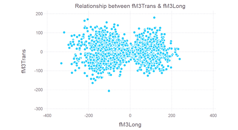
Figure 7.4 A scatter plot for features 7 and 8. Clearly there is little relationship (if any at all) between the fM3Long and fM3Trans variables.

You can create a scatter plot between two features in our dataset, like the one in Figure 7.4, using the following code:

In[13]: plot(x = df[:fM3Long], y = df[:fM3Trans], Geom.point, Guide.xlabel(“fM3Long”), Guide.ylabel(“fM3Trans”), Guide.title(“Relationship between fM3Trans & fM3Long”))

Scatter plots using the output of t-SNE algorithm

It is truly fascinating how this simple yet brilliant algorithm developed by the Dutch scientist Laurens van der Maaten is rarely mentioned in data science books and tutorials. It has been used extensively in the data exploration of large companies like Elavon (US Bank) and Microsoft. Prof. Van der Maaten’s team has implemented it in most programming platforms, including Julia, so there is no excuse for ignoring it! You can find the latest package here: http://bit.ly/29pKZUB. To install it, clone the package on your computer using the following command, as it is not an official package yet:

In[14]: Pkg.clone(“git://github.com/lejon/TSne.jl.git”)

In short, t-SNE is a mapping method that takes a multi-dimensional feature space and reduces it to 1, 2 or 3 dimensions. From here, the data can be plotted without having to worry about distorting the dataset’s geometrical properties in the process.

It was first introduced to the scientific world in 2008 through a couple of papers, the most important of which was published in the Journal of Machine Learning Research and can be read at http://bit.ly/29jRt4m. For a lighter introduction to this piece of technology, you can check out Professor Van der Maaten’s talk about his algorithm on YouTube: http://bit.ly/28KxtZK.

For our dataset we can get a good idea of how its data points relate to the two classes by examining the resulting plot, which looks like something similar to the one in Figure 7.5 (we say “similar” because every time you run the algorithm it will produce slightly different results, due to its stochastic nature).

Figure 7.5 A scatter plot based on the output of the t-SNE algorithm on the magic dataset. You can view the plot in full color online at http://bit.ly/1LW2swW.

This plot clearly indicates that there is a significant overlap between the two classes, making classification a challenging task. The h class is more or less distinct in some regions of the feature-space, but for the most part g and h are interlaced. Therefore, it would behoove us to apply a more sophisticated algorithm if we want a good accuracy rate for this dataset.

Although the method is ingenious, the documentation of its Julia implementation remains incomplete. Here is how you can use it without having to delve into its source code to understand what’s going on:

1. Normalize your dataset using mean and standard deviation.

2. Load the tSNE package into memory using tsne().

3. Run the main function: Y = tsne(X, n, N, ni, p), where X is your normalized dataset, n is the number of dimensions that you wish to reduce it to (usually 2), N is the original number of dimensions, ni is the number of iterations for the algorithm (default value is 1000), and p is the perplexity parameter (default value is 30.0).

4. Output the result:

In[14]: labels = [string(label) for label in O[1:length(O)]]

In[15]: plot(x = Y[:,1], y = Y[:,2], color = labels)

If you are unsure of what parameters to use, the default ones should suffice; all you’ll need is your dataset and the number of reduced dimensions. Also, for larger datasets (like the one in our example) it makes sense to get a random sample as the t-SNE method is resource-hungry and may take a long time to process the whole dataset (if it doesn’t run out of memory in the meantime). If we apply t-SNE to our dataset setting n = 2 and leaving the other parameters as their default values, we’ll need to write the following code:

In[16]: using TSne

In[17]: include(“normalize.jl”)

In[18]: include(“sample.jl”)

In[19]: X = normalize(X, “stat”)

In[20]: X, O = sample(X, O, 2000)

In[21]: Y = tsne(X, 2)

In[22]: plot(x = Y[:,1], y = Y[:,2], color = O)

In our case the labels (vector O) are already in string format, so there is no need to create the labels variable. Also, for a dataset of this size, the t-SNE transformation is bound to take some time (the tsne() function doesn’t employ parallelization). That’s why in this example we applied it to a small sample of the data instead.

Scatter plots are great, especially for discreet target variables such as classification problems. For different types of problems, such as regression scenarios, you could still use them by including the target variable as one of the depicted variables (usually y or z). In addition, it is best to normalize your variables beforehand, as it is easy to draw the wrong conclusions about the dataset otherwise.

Histograms

Histograms are by far the most useful plots for data exploration. The reason is simple: they allow you to see how the values of a variable are spread across the spectrum, giving you a good sense of the distribution they follow (if they do follow such a pattern). Although useful, the normal distribution is rather uncommon, which is why there are so many other distributions created to describe what analysts observe. With Julia you can create interesting plots depicting this information, like the one shown in Figure 7.6.

Figure 7.6 A histogram of feature 9 (fAlpha). Clearly this feature follows a distribution that is nowhere near normal.

You can get Julia to create a histogram like this one by using the following code:

In[23]: p = plot(x = df[:fAlpha], Geom.histogram, Guide.xlabel(“fAplha”), Guide.ylabel(“frequency”))

If you want a coarser version of this plot with, say, 20 bins, you can add the bincount parameter, which by default has a rather high value:

In[24]: p = plot(x = df[:fAlpha], Geom.histogram(bincount = 20), Guide.xlabel(“fAplha”), Guide.ylabel(“frequency”))

From both versions of the histogram, you can see that the fAlpha variable probably follows the power law, so it has a strong bias towards smaller values (to be certain that it follows the power law we’ll need to run some additional tests, but that’s beyond the scope of this book).

Exporting a plot to a file

Exporting plots into graphics or PDF files is possible using the Cairo package. This is a C-based package that allows you to handle plot objects and transform them into three types of files: PNG, PDF, or PS. (Cairo may not work properly with early versions of Julia.) For example, we can create a nice .png and a .pdf of the simple plot myplot using the following code:

myplot = plot(x = [1,2,3,4,5], y = [2,3.5,7,7.5,10])

draw(PNG(“myplot.png”, 5inch, 2.5inch), myplot)

draw(PDF(“myplot.png”, 10cm, 5cm), myplot)

The general formula for exporting plots using Cairo is as follows:

draw(F(“filename.ext”, dimX, dimY), PlotObject)

In this code, F is the file exporter function: PNG, PDF, or PS, and filename.ext is the name of the desired image file. dimX and dimY are the dimensions of the plot on the X and Y axis, respectively. If they are left undefined, Julia assumes number of pixels, but you can also specify another unit of measurement, such as inches or cm, by adding the corresponding suffix. Finally, PlotObject is the name of the plot you want to export.

Alternatively, if you run your plotting script in the REPL you can save the created graphic from your browser, where it is rendered as an .html file. This file is bound to be larger than a typical .png but it is of lossless quality (since the plot is rendered whenever the page is loaded) and incorporates the zoom and scroll functionality of the Gadfly plots in the Julia environment. In fact, all the plots included in this chapter were created using this particular process in the REPL, attesting to the quality of browser-rendered plots.

Hypothesis Testing

Suppose you are a data scientist and you want to check whether your hypotheses about the patterns you see in your data (i.e. the particular variables you are focusing on) hold “true”. You notice that the sales variable is different at certain days of the week but you are not sure whether that’s a real signal or just a fluke. How will you know, and avoid wasting your manager’s valuable time and your expensive resources? Well, that’s why hypothesis testing is here.

Testing basics

In order to harness the power of hypothesis testing, let’s quickly review the theory. Hypothesis testing is an essential tool for any scientific process, as it allows you to evaluate your assumptions in an objective way. It enables you to assess how likely you are to be wrong if you adopt a hypothesis that challenges the “status quo.” The hypothesis that accepts the status quo is usually referred to as the null hypothesis, and it’s denoted H0. The proposed alternative is creatively named the alternative hypothesis, and it’s denoted H1.

The more you can convince someone that H1 holds “true” more often than H0, the more significant your test is (and your results, as a consequence). Of course you can never be 100% certain that H1 is absolutely “true”, since H0 has been considered valid for a reason. There is a chance your alternative hypothesis is backed by circumstantial evidence (i.e. you were lucky). Since luck has no place in science, you want to minimize the chances that your results were due to chance.

This chance is quantified as alpha (ɑ), a measure of the probability that your alternative hypothesis is unfounded. Naturally, alpha is also a great metric for significance, which is why it is the primary significance value of your test. Alpha values that correspond to commonly used significance levels are 0.05, 0.01, and 0.001. A significance of ɑ = 0.01, for example, means that you are 99% sure that your alternative hypothesis holds truer than your null hypothesis. Obviously, the smaller the alpha value, the stricter the test and therefore the more significant its results are.

Types of errors

There are two types of errors you can make through this schema:

• • Accept H1 while it is not “true”. This is also known as a false positive (FP). A low enough alpha value can protect you against this type of error, which is usually referred to as type I error.
• • Reject H1 even though it is “true”. Usually referred to as a false negative (FN), this is a usually a result of having a very strict significance threshold. Such an error is also known as a type II error.

Naturally you’ll want to minimize both of these types of errors, but this is not always possible. The one that matters most depends on your application, so keep that in mind when you are evaluating your hypotheses.

Sensitivity and specificity

Sensitivity is the ratio of correctly predicted H1 cases to total number of H1 cases. Specificity is the ratio of correctly predicted non-H1 cases to total number of non-H1 cases. In practice, these two metrics are variables that we calculate. These variables are not arbitrarily large or small, since they cannot be larger than 1 or smaller than 0. This is often expressed as “taking values in” a given interval. So, here is how the four distinct cases of a test result relate to sensitivity and specificity:

Test Result	Relationship to S & S
true positive result (correctly predicted H1 cases)	sensitivity
false negative result (missed H1 cases)	1-sensitivity
true negative result (H0 cases predicted as such)	specificity
false positive result (H0 cases predicted as H1 ones)	1-specificity

Table 7.1 The relationship between sensitivity and specificity and corresponding test results.

We will come back to sensitivity and specificity when we’ll discuss performance metrics for classification, in Chapter 9.

Significance and power of a test

These concepts are useful for understanding the value of a test result, although they provide little if any information about its importance. That’s something that no statistical term can answer for you, since it depends on how much value you bring to your client.

Significance, as we saw earlier, is how much a test’s result matters–a sign that the result is not some bizarre coincidence due to chance. It is measured with alpha, with low alpha values being better. So, if your test comes up with what is called a p value (the probability that we obtain this result by chance alone) that is very small (smaller than a predetermined threshold value of alpha, such as 0.01), then your result is statistically significant and possibly worth investigating further. You can view significance as the probability of making a type I error.

Similarly, you can consider the power of a test as the chance that a test would yield a positive result, be it a true positive or a false positive. Basically, it’s the probability of not making a type II error. Naturally, you would want your test to have a small value for significance and a high value for power.

Kruskal-Wallis tests

The Kruskal-Wallis (K-W) test is a useful statistical test that checks the levels of a factor variable to see whether the medians of a corresponding continuous variable are the same, or at least one pair of them is significantly different. Such a test is particularly handy for cases like in the magic dataset, when the target variable is a nominal one; it is usually even more applicable in cases where there are several different values (at least three).

In general, you’d apply the K-W test using the following function of the HypothesisTests package:

KruskalWallisTest{T<:Real}(g::AbstractVector(T))

where g is a one-dimensional array (or AbstractVector) comprising the groups of the continuous variable that is tested.

You can learn more about the K-W test by reading the documentation created by the Northern Arizona University, found at http://bit.ly/28OtqhE. If you wish to dig deeper, we recommend Prof. J. H. McDonald’s excellent website on biostatistics, found at http://bit.ly/28MjuAK.

T-tests

One of the most popular techniques to test hypotheses is the t-test. This type of statistical test enables you to compare two samples (from the same variable) and see if they are indeed as different as they appear to be. One of its main advantages is that it can handle all kinds of distributions, while it is also easy to use (compared to some statistical tests that require a prerequisite training course in statistics). That’s one of the reasons why the t-test is one of the most commonly encountered tests out there, especially for continuous variables.

Let’s consider two examples of the same variable sales we discussed in our hypothetical case at the beginning of the section. We can plot their distributions as in Figure 7.7. They need not be so neat, since we make no assumptions about the distributions themselves—as long as the number of data points is more than 30. Still, the plot alone cannot answer our question: are the sales on the two different days different enough to be considered a signal or is it just noise–random fluctuations due to chance?

Figure 7.7 The distributions of two sets over a given variable. Although the two samples appear to be different (their means are not the same), this can only be confirmed through the use of a statistical test, such as the t-test.

Fortunately, the t-test can give us the answer to this question, along with a measure of how likely it is to be wrong (alpha value). Julia can work a t-test as follows, depending on whether the variances of the two distributions are the same:

pvalue(EqualVarianceTTest(x, y))

pvalue(UnequalVarianceTTest(x, y))

where x and y are one-dimensional arrays containing the data samples in question.

Of course, we can split our data in a zillion different ways. One meaningful distinction is based on the class variable. This way we can see if a particular continuous feature is different when it applies to the data points of class g compared to the data points of class h. Before we run the test, we need to split the data into these two groups, and then compare their variances. In this example we’ll look at the 10th feature (fDist), but the same process can be applied to any feature in this dataset.

In[25]: ind1 = findin(df[:class], [“g”])

In[26]: ind2 = findin(df[:class], [“h”])

In[27]: x_g = df[:fDist][ind1]

In[28]: x_h = df[:fDist][ind2]

In[29]: v_g = var(x_g)

In[30]: v_h = var(x_h)

It’s now clear that the two samples are different in variance; the second sample’s variance is about 36% more than the first sample’s. Now we’ll need to apply the second variety of the t-test, when the variances of the two distributions are not the same:

In[31]: pvalue(UnequalVarianceTTest(x_g, x_h))

The result Julia returns is an exceptionally small number (~7.831e-18), which indicates a very low probability that this difference in means is due to chance. Needless to say, that’s significant regardless of the choice of alpha (which can take values as small as 0.001, but rarely smaller). In other words, there’s a better chance that you’ll be struck by a lightning three times in a row than that the means of this feature are different by chance alone (according to the National Lightning Safety Institute, the chances of getting struck by a lightning, in the US, are about 1 in 280000, or 0.00035%.) The impact of this insight is that this feature is bound to be a good predictor, and should be included in the classification model.

Chi-square tests

The chi-square test is the most popular statistical test for discreet variables. Despite its simplicity, it has a great mathematical depth (fortunately, you won’t have to be a mathematician in order to use it). Despite the somewhat complex math involved, a chi-square test answers a relatively simple question: are the counts among the various bins as expected? In other words, is there any imbalance in the corresponding distributions that would suggest a relationship between the two discreet variables? Although such a question can occasionally be answered intuitively (particularly when the answer is significantly positive), it is difficult to assess the borderline case without a lot of calculations. Fortunately Julia takes care of all the math for you, through the following function from StatsBase:

ChisqTest(x, y)

where x and y are rows and columns, respectively, of a contingency table of two variables. Alternatively, you can pass to Julia the whole table in a single variable X, which is particularly useful when tackling more complex problems where both variables have three or more unique values:

ChisqTest(X)

Since we don’t have any discreet variables in our dataset, we’ll create one for illustration purposes, based on the fLength feature. In particular, we’ll break it up into three bins: high, medium, and low, based on an arbitrary threshold. The high bin will include all data points that have a value greater than or equal to μ + σ; the low bin will contain anything that is less than or equal to μ - σ; all the remaining points will fall into the medium bin.

Try this out as an exercise in data-wrangling. Use the .>= and .<= operators for performing logical comparison over an array; to find the common elements of two arrays, along with the intersect() function. With some simple logical operations we end up with the contingency table shown in Table 7.2.

Class / fLength	Low	Medium	High	Total
g	0	11747	585	12332
h	34	4778	1876	6688
Total	34	16525	2461	19020

Table 7.2 A contingency table showing counts of “Low”, “Medium,” and “High” values of the fLength feature, against the class variable.

Based on the above data (which is stored in, say, the two-dimensional array C, comprising of the values of the first 2 rows and the first 3 columns of the table), we can apply the chi-square test as follows:

In[32]: ChisqTest(C)

Julia will spit out a lot of interesting but ultimately useless information regarding the test. What you need to focus on is the summary that’s buried somewhere in the test report:

Out[32]: Test summary:

    outcome with 95% confidence: reject h_0

    two-sided p-value:   0.0 (extremely significant)

Clearly there is no way that these counts could have been generated by chance alone, so we can safely reject the null hypothesis (which Julia refers to as h_0) and conclude that there is a significant relationship between fLength and the class variable. Again, this means that we may want to include it (or the original feature it was created from) in our model.

The result of the chi-square test will not always be so crystal clear. In these cases, you may want to state beforehand what your significance threshold (alpha) will be and then compare the p-value of the test to it. If it’s less than the threshold, you can go ahead and reject the null hypothesis.

Other Tests

Apart from the aforementioned tests, there are several others that are made available through the HypothesisTests package. These may appeal to you more if you have a mathematical background and/or wish to discover more ways to perform statistical analysis using Julia. We encourage you to explore the package’s excellent documentation (http://hypothesistestsjl.readthedocs.org) and practice any of the tests that pique your interest. You can find additional information about the various statistical tests at reputable Stats websites, such as http://stattrek.com.

Statistical Testing Tips

The world of statistical testing is vast, but by no means exhaustive. That’s why it’s been a fruitful field of research since its inception. As the realm of big data makes these techniques more valuable, its evolution is bound to continue. Still, the tests mentioned in this chapter should keep you covered for the majority of the datasets you’ll encounter. Remember that there is no “perfect score” for a given problem; it is not uncommon for someone to try out several statistical tests on her data before arriving at any conclusions. Furthermore, the results of these tests are better used as guidelines than strict rules. Often, a pair of variables may pass a certain test but fail others, so they definitely cannot be a substitute for human judgment. Instead, they can be useful tools for drawing insights and supporting your own intuitions about the data at hand.

Case Study: Exploring the OnlineNewsPopularity Dataset

We will practice applying all of these tools on another dataset, start to finish. We’ll return to the previously mentioned OnlineNewsPopularity dataset, which is a classic case of a regression problem. As we saw in Chapter 2, this problem aims to predict the number of shares of various online news articles based on several characteristics of the corresponding posts. This is particularly important for the people creating these articles, as they want to maximize their impact in social media. Let’s first load it into a dataframe, for more intuitive access to its variables (which in this case are already in the .csv file as a header):

In[33]: df = readtable(“OnlineNewsPopularity.csv”, header = true)

By examining a few elements of this dataframe it becomes clear that the first variable (url) is just an identifier, so we have no use for it in our models, nor in the exploratory part of our analysis.

Variable stats

Now let’s dig into the various descriptive statistics of our dataset, including the target variable:

In[34]: Z = names(df)[2:end]  #1

In[35]: for z in Z

    X = convert(Array, df[symbol(z)]);

    println(z, “ ”, summarystats(X))

  end

#1 Exclude the first column of the data frame (url) as it is both non-numeric and irrelevant

From all these, it is clear that the variables’ values are all over the place, so we should go ahead and normalize them as we saw in the previous chapter:

In[36]: for z in Z

    X = df[symbol(z)]

    Y = (X - mean(X)) / std(X) #1

    df[symbol(z)] = Y

  end

#1 This is equivalent to normalize(X, “stat”), which we saw earlier.

Other than that, there is nothing particularly odd about the variables that begs any additional work. One thing to keep in mind is that some of the variables are binary, even though they are coded as floats in the data frame. We don’t need to normalize the features since they are already on the same scale as the other (normalized) features. There are no consequences.

Before we move on to the visualizations, let’s see how the different variables correlate with the target variable:

In[37]: n = length(Z)

In[38]: C = Array(Any, n, 2)

In[39]: for i = 1:n

      X = df[symbol(Z[i])]

      C[i,1] = Z[i][2:end]

      C[i,2] = cor(X, df[:shares])

    end

The above code produces a two-dimensional array that contains the names of the variables and their corresponding correlation coefficients with the target variable (shares). Clearly the relationships are all weak, meaning that we’ll need to work harder to build a decent prediction model for this dataset.

Visualization

All that statistical talk is great, but what do our features look like and how do they compare with the target variable? Let’s find out with the following code:

In[40]: for i = 1:n

  plot(x = df[symbol(Z[i])], Geom.histogram,  Guide.xlabel(string(Z[i])), Guide.ylabel(“frequency”))

  plot(x = df[symbol(Z[i])], y = df[:shares], Geom.point,  Guide.xlabel(string(Z[i])), Guide.ylabel(“shares”))

   end

The result is a series of histograms accompanied by scatter plots with the target variable, a few of which are shown in Figure 7.8.

Figure 7.8 Histograms of the first three variables, and scatter plots between them and the target variable.

The histograms indicate that the majority of the features don’t have particularly strong relationships with the target variable, although there is some signal there. This confirms the correlations (or lack thereof) we calculated in the previous paragraph.

Hypotheses

Clearly the traditional approach to hypothesis creation and testing we discussed previously won’t apply here, since we don’t have a discreet target variable. However, with a little imagination we can still make use of the t-test, bypassing the limitations of any distribution assumptions. We can split the target variable into two parts (high and low values) and see whether the corresponding groups of values of each variable are significantly different.

This is similar to the correlation coefficient approach, but more robust, as it doesn’t search for a linear relationship (which would have been pinpointed by the correlation coefficient). The big advantage is that it manages to show whether there is an underlying signal in each variable, without getting too complicated. (The next level of complexity would be to run ANOVA and MANOVA models, which go beyond the scope of data exploration.) So, let’s see how the HypothesisTests package can shed some light onto this dataset through the code in listing 7.1:

In[41]: a = 0.01                #1

In[42]: N = length(Y)

In[43]: mY = mean(Y)

In[44]: ind1 = (1:N)[Y .>= mY]

In[45]: ind2 = (1:N)[Y .< mY]

In[46]: A = Array(Any, 59, 4)

In[47]: for i = 1:59

     X = convert(Array, df[symbol(Z[i])])

     X_high = X[ind1]

     X_low = X[ind2]

     var_high = var(X_high)

     var_low = var(X_low)

     if abs(2(var_high - var_low)/(var_high + var_low)) <= 0.1 #2

      p = pvalue(EqualVarianceTTest(X_high,X_low))

     else

      p = pvalue(UnequalVarianceTTest(X_high,X_low))

     end

     A[i,:] = [i, Z[i], p, p < a]

     if p < a

      println([i, “ ”, Z[i]]) #3

     end

   end

#1 Set the significance threshold (alpha value)

#2 Check to see if variances are within 10% of each other (approximately)

#3 Print variable number and name if it’s statistically significant

Listing 7.1 A code snippet to apply t-tests to the OnlineNewsPopularity dataset.

Clearly the majority of the variables (44 out of 59) can accurately predict whether the target variable is high or low, with 99% certainty. So, it has become clear that the variables of the dataset are not so bad in terms of quality overall; they just don’t map the target variable in a linear manner.

T-SNE magic

Although t-SNE was designed for visualization of feature spaces, mainly for classification problems, there is no reason why we cannot apply it in this case–with a small twist. Instead of mapping the dataset onto a two- or three-dimensional space, we can use t-SNE on a one-dimensional space. Although this would be completely useless for visualization, we can still use its output in a scatter plot with the target variable and check for any type of relationship between the two. This will become more apparent once you try out the code snippet in Listing 7.2.

In[48]: using(“normalize.jl”)

In[49]: X = convert(Array, df)

In[50]: Y = float64(X[:,end])

In[51]: X = float64(X[:,2:(end-1)])

In[52]: X = normalize(X, “stat”)

In[53]: Y = normalize(Y, “stat”)

In[54]: X, Y = sample(X, Y, 2000)

In[55]: X1 = tsne(X, 1)

In[56]: plot(x = X1[ind], y = Y[ind], Geom.point)

Listing 7.2 Code snippet to apply t-SNE to the OnlineNewsPopularity dataset.

This code produces a highly compressed dataset (X1) that summarizes the whole normalized dataset into a single feature, and then plots it against the target variable (which we call Y in this case). This result is shown in Figure 7.9. Although the relationship between the inputs (X1) and the target is weak, it is evident that smaller values of X1 generally yield a slightly higher value in Y.

Figure 7.9 Scatter plot of T-SNE reduced dataset against target variable.

Conclusions

Based upon all of our exploratory analysis of the OnlineNewsPopularity dataset, we can reasonably draw the following conclusions:

• • The distributions of most of the variables are balanced.
• • Normalizing the variables is imperative.
• • There is a weak linear relationship between each input variable and the target variable.
• • The inputs of the dataset can predict whether the target variable is generally high or low, with statistical significance (a = 0.01).
• • Using a scatter plot based on t-SNE, we can see that the relationship of all the input variables with the target variable is reversely proportional (albeit weakly).

Summary

• • Data exploration is comprised of many different techniques. The most important of these are descriptive statistics (found in the StatsBase package), plots (Gadfly package), and hypothesis formulation and testing (HypothesisTests package).

Descriptive Statistics:

• • You can uncover the most important descriptive statistics of a variable x using the StatsBase package, by applying the following functions:
• ◦ summarystats(x) – This function is great for storing the stats into an object, so that you can use them later.
• ◦ describe(x) – This function is better for getting an idea of the variable through the display of the stats on the console.
• • You can calculate the correlation between two variables using one of the functions that follow:
• ◦ cor(x, y) – The Pearson method is best suited to distributions that are normal.
• ◦ corspearman(x, y) – The Spearman method will work with any kind of distribution.
• ◦ corkendall(x, y) – Kandell’s tau method is also good for any kind of distribution.
• • To create a correlation table with all possible correlations among a dataset’s variables, apply one of the above correlation functions with a single argument, the dataset array.

Plots:

• • There are several packages in Julia for plots, the most important of which are: Gadfly, Plotly, Bokeh, Winston, and Vega.
• • Before creating any visuals with Gadfly, it is best use a data frame to store all your variables.
• • In all Gadfly plots, you can label your creations using the following parameters in the plot() function:
• ◦ Guide.xlabel(“Name of your X axis”).
• ◦ Guide.ylabel(“Name of your Y axis”).
• ◦ Guide.title(“Name of your plot”).
• • You can create the following plots easily using Gadfly:
• ◦ Bar plot: plot(DataFrameYouWishToUse,
  x = “IndependentVariable”, Geom.bar).
• ◦ Line plot: plot(DataFrameYouWishToUse,
  y = “DependentVariable”, Geom.line).
• ◦ Scatter plot: plot(x = DataFrameName[:IndependentVariable],
  y = DataFrameName[:DependentVariable], Geom.point).
• ◦ Histogram: plot(x = DataFrameName[:VariableName], Geom.histogram).
• • You can visualize a whole dataset regardless of its dimensionality using the t-SNE algorithm in the tSNE package.
• • You can save a plot you have created and stored in an object using the Cairo package. Alternatively, you can screen capture the plot, or run the command on the REPL and save the HTML file it creates in your web browser.

Hypothesis Testing:

• • Hypothesis tests are a great way to reliably test an idea you may have about the relationships between variables. They can be run using tools in the HypothesisTests package. The most commonly used hypothesis tests are the following:
• ◦ t-test: pvalue(EqualVarianceTTest(x, y)), or in the case of different variances in your variables, pvalue(UnequalVarianceTTest(x, y)).
• ◦ chi-square test: ChisqTest(X).
• • Hypothesis tests are evaluated based on two factors, neither of which map the value of the results. Instead they show the scientific validity of the test. These factors are the following:
• ◦ Significance (alpha): The probability that your test makes a type I error. Significance is usually defined as thresholds corresponding to the alpha values of 0.05 (most common), 0.01, and 0.001 (least common).
• ◦ Power: The probability of not making a type II error. Power corresponds to how likely it is that your test yields a positive result (which can be either correct or incorrect).
• • Apart from the t-test and the chi-square test, there are several other statistical tests you can use; these are described in detail in the HypothesisTests documentation.

Chapter Challenge

1. 1. What action could be taken based on the identification of high correlation between two variables in a dataset?
2. 2. When can you prove the null hypothesis in a test?
3. 3. In a classification problem, under which conditions can you use correlation to see how well a feature aligns with the class variable?
4. 4. Explore a dataset of your choice and note down any interesting findings you come up with.
5. 5. Can a t-test be applied on variables following irregular distributions?
6. 6. Suppose we have a medical dataset comprising data of 20 patients. Can we draw any statistically significant conclusions about its variables using the standard test? Why?
7. 7. What would be the best plot to use for depicting a dataset’s feature space?
8. 8. What is the main use case for the t-SNE function?