
Modal and Non-modal Dialogs: What Is the Difference?
Navigating Reports Programmatically
Defensive Programming Strategies
As you become more proficient in JSL, there are some tools and concepts that will help you along the way. In this chapter, we discuss the following:
● building user dialogs that wait for user input, or not
● using programmatic methods for navigating your reports
● understanding the mysterious ways of expression functions
● making your scripts more robust
When you need to create a script to ask the user for a response or choice, use a dialog window. There are a couple of options available in JMP scripting to do the work. We explain the basics here.
The two main types of dialog windows are modal and non-modal. A modal window halts the script and waits until the user gives a response before the script execution continues. In contrast, for a non-modal window, the script does not wait for a response from the user. The window remains open until requested to close. Responses made by the user might initiate another section of script execution or other actions. Examples of non-modal windows include the built-in analysis windows in JMP.
The New Window() function offers both modal and non-modal options, which are explored in the following sections, as well as another modal option, Column Dialog().
New Window(): Modal
Use the modal option for the New Window() function when you need to force the script to stop and wait for a response from the script user.
For example, suppose you are developing a JMP script that surveys users about the types of pets they own. Start the script with a New Window() command. The basic syntax looks like this with the modal message added:
nw = New Window( title,<<Modal, displaybox );
We set up our display to ask the user a question with a text box and show the choices for answers in a list box. A horizontal list box is used to align the Text Box and List Box.
nw = New Window( "Pet Survey",
   <<Modal,
   H List Box(
       Text Box(
           "What type pets do you currently own?  Select all that apply."
       ),
        lb1 = List Box(
           {"Horse", "Dog","Cat", "Rodent","Pig", "Goat",
            "Llama or Alpaca", "Other Exotic"}
       )
   )
);
This script looks pretty good so far, but how do you retrieve the results and use them? You have a couple of options.
1. Add the Return Result message, and then subscript the new window reference:
nw = New Window( "Pet Survey",
   <<Modal,
   <<Return Result,
      H List Box(
       Text Box(
           "What type pets do you currently own?  Select all that apply."
       ),
        lb1 = List Box(
           {"Horse", "Dog","Cat", "Rodent","Pig", "Goat",
            "Llama or Alpaca", "Other Exotic"}
       )
   )
);

Show( nw["lb1"] );
2. Use a Button Box script to get the selected results. When the user clicks the OK button, the results are placed in the variable named results:
nw = New Window( "Pet Survey",
    <<Modal,
      H List Box(
       Text Box(
           "What type pets do you currently own?  Select all that apply."
       ),
        lb1 = List Box(
           {"Horse", "Dog","Cat", "Rodent","Pig", "Goat",
            "Llama or Alpaca", "Other Exotic"}
       ),
        Button Box( "OK", results = lb1 << Get Selected ),
        Button Box( "Cancel" )
    )
);

Show( results);
You might have noticed that we did not script an OK button in the first example. That is because JMP automatically adds a simple OK button to a modal dialog window if you do not.
When using the modal option with New Window(), there are other special options available. Please see the JSL Syntax Reference or the Scripting Guide for more information about these features.
New Window: Non-modal
The non-modal window does not halt the script action waiting for a response. Any code after the New Window() script is executed immediately.
Using the pet survey example again, we ask the survey respondent the same question as before regarding what type pets the user owns. Instead of an OK button, we will use a Submit button that, when clicked, gets the selected items as in the modal dialog. We also add a script to create yet another non-modal window that queries the user for any additional comments about the survey. Notice that all commands to print to the log are within Button Box scripts. If you place these commands after the main New Window() statement, they will be executed prior to getting the results of your survey.
As with the modal example, horizontal and vertical list boxes strategically wrap the display boxes to provide a more pleasing arrangement for the user interface.
Notice that both the Submit and Cancel buttons use << Close Window messages in this non-modal window example. The modal dialog window buttons perform this action automatically.
nw = New Window( "Pet Survey",
    H List Box(
        Text Box(
"What type pets do you currently own?  Select all that apply."
 ),
         lb1 = List Box(
{"Horse","Dog", "Cat","Rodent", "Pig","Goat",
 "Llama/alpaca", "Reptile"} ),
         V List Box(
             Button Box( "Submit Survey",
                 results = lb1 << Get Selected;
                 Print( results );
                 nw << Close Window;
                 AddComment = New Window( "Comments",
                     H List Box(
                        Text Box(
    "Comments about this survey? Please add: "
 ),
                        teb = Text Edit Box( "  <comments>  " ),
                        V List Box(
                            Button Box( "Submit",
                                userComment = teb << get text;
                                Print( userComment );
                                addComment << Close Window;
                           ),
                           Button Box( "Cancel",
    Add Comment << Close Window
  )
                       )
                    )
                );
            ),
            Button Box( "Cancel", nw << Close Window )
        )
    )
);
The New Window() function offers many more options than are shown here. Please see the JSL Syntax Reference or the Scripting Guide for more information about these features. Additional examples of using New Window() are in chapter 8 of this book, “Dialog Windows.”
Column Dialog() is a specialized modal dialog function that presents the user with a dialog window with the columns of the current data table. If you need a launch window to prompt users to cast columns in roles, this function is for you.
The main display component of Column Dialog() is the ColList() element, but this window also accommodates container boxes for display, such as list boxes, check boxes, and radio buttons. You can specify the minimum and maximum columns to be cast in for each variable, as well as the data types and modeling types. There is no need to script buttons, as this is a modal dialog with the buttons already built in.
colDlg = Column Dialog(
   gb_y = ColList( "Temperature Variables",
          Min Col( 1 ),
          Max Col( 3 ),
          Data Type( "Numeric" )
   ),
   gb_x = ColList( "Date", Max Col( 1), Data Type( "Numeric" ), )
);
Show(colDlg);
What is returned after running the dialog script might look like this, if the :TMIN, :TMAX, :TAVG, and :Date columns were selected and the OK button was clicked:
colDlg = {gb_y = {:TMIN, :TMAX, :TAVG}, gb_x = {:DATE}, Button(1)};
Note: If the Cancel button was clicked instead, Button(-1) would be returned, and the variables gb_y and gb_x would be empty lists.
To use the results from a modal dialog window, you must reference the values by subscripting the list result to use elsewhere in the script. But first, remove the last item in the list, Button(1), and then evaluate the list:
Remove From( coldlg, N Items( coldlg ) ););
Show( colDlg );
colDlg = {gb_y = {:TMIN, :TMAX, :TAVG}, gb_x ={:DATE}};
Eval List( coldlg );
Show( gb_y, gb_x );
gb_y = {:TMIN, :TMAX, :TAVG};
gb_x = {:DATE};
Now you are ready to use your variable in your scripted platform.
Keep in mind you can also script your own column dialog from scratch using the New Window() function, which offers more options. However, the Column Dialog() function is quick and easy.
For more information about syntax and options, reference the Scripting Index. See chapter 8 for another example of a column dialog window.
In chapter 3, we discussed platform objects and how they are constructed. Specifically, we showed that the resulting reports consist of two layers: the analysis layer and the report layer. In each of the examples discussed, we used a subscripting method to retrieve values, change axis settings, and add or remove items from a report. Let’s dive a little deeper into navigating reports using subscripting and explore XPath as an alternative for locating items in the XML representation of a report.
In JSL, subscripting is useful for accessing values in various objects, such as columns, lists, matrices, and display boxes. Since the report layer consists of display boxes, subscripting is an easy way to reference items in a report.
When you look at the Tree Structure window, you will notice that most items have a number in parentheses after the display box name. Using these numbers is not a reliable method for referencing specific display boxes, because the numbers can be affected by a variety of things, such as preference settings and the version of JMP being used.
A more robust approach is to subscript the report by the title of the Outline Box that is the container for the desired value. This method is known as relative referencing. The desired value can be accessed in relation to that Outline Box as a subscript.
In chapter 3, we discussed extracting the R-squared value from a Oneway report. In that example, we referenced the Number Col Box that contained the R-squared value as a subscript of the Summary of Fit Outline Box title. However, the number shown in the tree structure for the Number Col Box happened to be the same as we used in our script. That will not always be the case. So let’s look at a different example that exposes the problem with using the display box number shown in the tree structure.
Suppose you wanted to extract the height estimate from the Parameter Estimates table in a Bivariate report. We will begin by looking at the tree structure. Since we are specifically interested in Parameter Estimates, we can right-click the gray disclosure icon beside Parameter Estimates, and select Edit► Show Tree Structure to see only the part of the tree structure that pertains to the Parameter Estimates Outline Box .
Figure 7.1 Parameter Estimates and Tree Structure
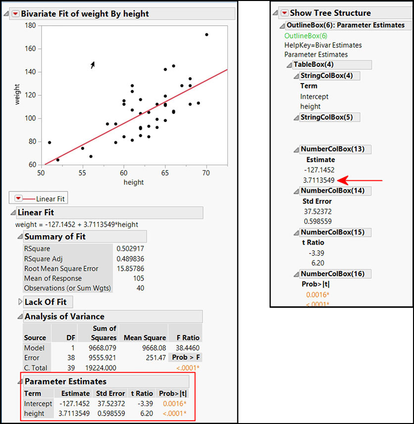
Based on what we learned in chapter 3, the proper way to access the height estimate would be to first access the report layer. To use relative referencing, we then subscript using the title of the Parameter Estimates Outline Box, followed by the Number Col Box in relation to the Outline Box, and the location of the value in that Number Col Box.
That script would look like this:
dt = Open("$SAMPLE_DATABig Class.jmp");

biv = dt << Bivariate(
   Y( :weight ),
   X( :height ),
   Fit Line
);

heightEstimate =                 //Assign a variable to the result
 Report( biv )                  //Report Layer
      ["Parameter Estimates"]    //"Parameter Estimates" Outline Box
          [Number Col Box( 1)]  //First NumberColBox
              [2];               //Second item

Show( heightEstimate );
/*:
heightEstimate = 3.71135489385953;
By using the string "Parameter Estimates" as the first subscript, we directed JMP to that Outline Box, regardless of what number is shown for Outline Box(n) in the tree structure.
Though the tree structure shows NumberColBox(13) in Figure 7.1, the Number Col Box is the first Number Col Box under the Parameter Estimates Outline Box. Therefore, Number Col Box( 1 ) is the next subscript.
The last subscript, [2], refers to the second item in that Number Col Box, which is the actual value that we wanted.
|
Look at the GIF file named Chapter7_SubscriptDemo.gif, included in the files that accompany this book, to see a visual demonstration of the items subscripted. |
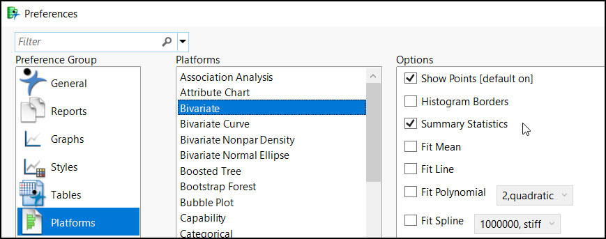
Now, what would happen if another user ran this same script but had different preference settings? Suppose the user has turned on the Summary Statistics preference.
Figure 7.2 Bivariate Preferences
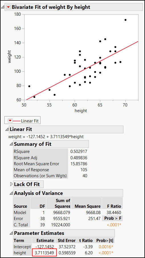
Because we subscripted by the Parameter Estimates Outline Box title, the script will produce the report and extract the correct value, as shown in Figure 7.3.
Figure 7.3 Report and Log
|
|
dt = Open("$SAMPLE_DATABig Class.jmp");
biv = dt << Bivariate(
       Y( :weight ),
       X( :height ),
       Fit Line
);
//Assign a variable to the result
heightEstimate =
  //Report Layer
  Report( biv )
      //Outline Box  Title
      ["Parameter Estimates"]
          //First NumberColBox
          [Number Col Box( 1 )]
              //Second item
              [2];

Show( heightEstimate );
/*:
heightEstimate = 3.71135489385953; |
If we had not used relative referencing and instead used NumberColBox(13)as shown in the tree structure, JMP would have attempted to extract a value from a Number Col Box in the Lack Of Fit report table instead of the Parameter Estimates report table.
Figure 7.4 Report and Tree Structure with Summary Statistics
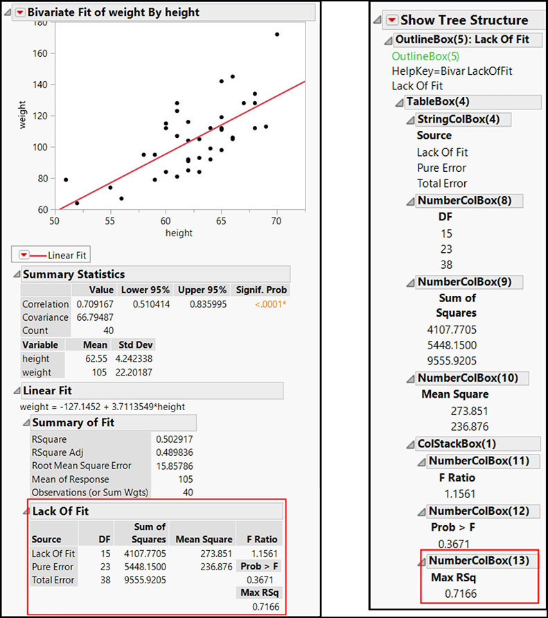
Notice that there is only one item in this NumberColBox(13). Therefore, an error is generated in the log when we attempt to subscript to an item that does not exist.
dt = Open( "$SAMPLE_DATABig Class.jmp" );

biv = dt << Bivariate(
   Y( :weight ),
   X( :height ),
   Fit Line
);

heightEstimate = Report( biv )[Number Col Box(13 )][2];
/*:
index in access or evaluation of 'Get' , Get( 2 ) /*###*/
As this example demonstrates, relative referencing ensures that your script runs correctly even when another JMP user has different preference settings. This is one reason relative referencing is considered a best practice and overall good scripting habit.
Another way to prevent preferences from affecting how your script behaves is to add the Ignore Platform Preferences( 1 ) option to your platform call. Although you can probably think of instances where this option would be useful, it might be undesirable. For any options that the user prefers to appear in the report (or not, as the case may be), the user would have to make those changes either to the script or interactively.
As stated earlier, preferences are only one reason the display box numbering could be different from what you expect at the time you create your script. Because JMP is always improving and listening to customer requests and feedback, report structure might also differ between releases of JMP. By using relative referencing, you are guarding your script against the effects of those types of changes.
Many of us are familiar with XML documents. For those who are not, XML stands for Extensible Markup Language. It is a markup language that establishes a set of rules for documents that are readable and understood by machines. XPath is a query language that enables you to navigate your XML documents.
Though XML looks quite a bit like HTML, their purposes are different. The purpose of HTML is to display content, whereas the purpose of XML is more about data storage and conveying content.
Let’s discuss a few of the primary components of an XML document:
● Tags – Tags are what makes XML look a bit like HTML. Tags generally start with an opening less than sign (<) and end with a closing greater than sign (>). The tag name is specified between the < and > signs, and it is not a predefined value. Instead, the author of the document must establish the tag names. As in HTML, tags must be closed with a forward slash to represent an ending tag (for example, <tagname> content </tagname>).
● Elements – An element consists of an entire tag statement, if you will. An element begins with the < of the opening tag all the way to and including the > of the closing tag. Elements can contain other elements, as well.
● Attributes – Attributes are metadata or additional details about an element. An attribute is specified in the opening tag and can only have one value, specified in double quotation marks. A tag can have multiple attributes, but only one of each type.
● Content – Content is the data. It is the text, numbers, and other characters between the opening and closing tags that make up an element.
Consider the following example XML file. The openTables element is the root element in which all other elements appear. The table element has an attribute called current, which has a value of 0 or 1. Inside each table element are three additional elements: name, numCols, and numRows. The data appears between the tags.
<openTables>

   <table current="1">
          <name>Big Class</name>
          <numCols>5</numCols>
          <numRows>40</numRows>
   </table>

   <table current="0">
          <name>Fitness</name>
          <numCols>9</numCols>
          <numRows>31<numRows>
   </table>

</openTables>
Now that we understand the structure of an XML document, we can apply that knowledge to the structure of a JMP report as an XML document. To see the XML representation of a JMP report, send the Get XML message to the report layer. The XML will appear in the log (View ► Log).
|
|
A bit of warning: Do not be alarmed by the magnitude of the XML that appears in the log. It still has the same format of the preceding simple example, just with more elements, attributes, and content. |
Let’s look at an example. Suppose you wanted to programmatically determine how many Outline Boxes appeared in a Distribution report.
dt = Open("$SAMPLE_DATABig Class.jmp" );

dist = dt << Distribution(
   Stack( 1 ),
   Continuous Distribution(
          Column( :height ),
          Horizontal Layout( 1 ),
          Vertical( 0 )
   )
);
You could use JSL to step through the display boxes and check their type, but it would be a rather tedious task. Instead, let’s look at the XML representation.
Write( Report( dist ) << Get XML );
The result shown in the log is a string that is nearly 180 lines long. Don’t be overwhelmed! Scroll to the top of the log and look at just the first tag:
/*:
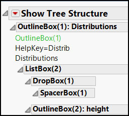
<OutlineBox width="717" height="277" helpKey="Distrib" isOpen="true">
The tag is named OutlineBox and it has four attributes: width, height, helpKey, and isOpen. Everything that comes next is the content of the element, which is the title of the Outline Box and other elements. As you look at the other elements, notice that the element names are the same as the display box names in the tree structure but in an XML format.
Figure 7.5 XML Elements Compared to Tree Structure
|
|
|
Now that we know the tag name of the element that we are searching for, let’s explore how we can use XPath to find out how many Outline Boxes there are.
|
|
As mentioned, XPath is a query language. It is not specific to JMP or JSL. Rather, there are many resources on the internet to help you understand all the details of XPath. In this book, we demonstrate some of the options available in XPath. |
In JMP, the XPath() message is sent to either the platform object or the report object. Its argument is an XPath expression used to retrieve information from the XML representation of the report. You do not have to use Get XML before you can use the XPath() message. But you might find it helpful to review the structure and available attributes.
The following will search the report for any Outline Boxes and return a list of references to each Outline Box.
obList = Report( dist ) << XPath("//OutlineBox" );
Show( obList );
/*:
obList = {DisplayBox[OutlineBox], DisplayBox[OutlineBox], DisplayBox[OutlineBox], DisplayBox[OutlineBox]};
We could simply use the NItems() function on obList to obtain the number of Outline Box references are stored in the list. Or as you learn more about the XPath language, you can use the XPath Count() function to return the count instead of a reference to each Outline Box.
obCount = N Items( Report( dist ) << XPath( "//OutlineBox") );
//OR
obCount = Report( dist ) << XPath( "count(//OutlineBox)");
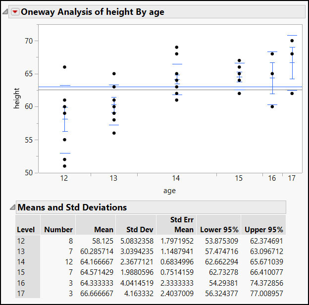
Now let’s look at a more interesting example. Suppose we wanted to display only the Mean and Std Dev columns in a Means and Std Deviations table of a Oneway report.
Figure 7.6 Oneway with Means and Std Deviations
|
|
dt = Open(
 "$SAMPLE_DATABig Class.jmp"
);

ow = dt << Oneway(
    Y( :height ),
    X( :age ),
    Means and Std Dev( 1 ),
    Mean Error Bars( 1 ),
    Std Dev Lines( 1 ),
    Mean of Means( 1 )
);
|
We can return a list of just the Number Col Box references under the Means and Std Deviations table using a combination of subscripting and XPath:
/* Return a list of NumberColBox references */
ncbList = Report( ow )["Means and Std Deviations"] << XPath( "//NumberColBox" );
Using a JSL For() loop, we can check the heading of the column and change the visibility property to collapsed if the heading is anything other than Mean or Std Dev.
/* Loop through each item to show only the Mean, Std Dev columns */
For( i = 1, i <= N Items( ncbList ), i++,
   rptColName = ncbList[i] << Get Heading;
   If( !Contains( {"Mean","Std Dev"}, rptColName ),
          ncbList[i]<< Visibility( "Collapse" )
   )
);
But again, there is a way in XPath to accomplish the same result without the need for the For() loop. Look at an excerpt of the XML representation of a Number Col Box from the report:
<NumberColBox leftOffset=!"40!" topOffset=!"0!" isVisible=!"false!">
<NumberColBoxHeader>Number</NumberColBoxHeader>
Notice that there is an element within the NumberColBox element called NumberColBoxHeader. This element contains the report column heading. XPath enables us to capture that text and perform comparisons. Only references to Number Col Boxes that have a heading that are anything other than Mean or Std Dev are returned in a list.
colsToHide = Report( ow )["Means and Std Deviations"] << XPath(
   "//NumberColBox[NumberColBoxHeader[not(text() = 'Mean')
and not(text() = 'Std Dev')]]"
);
This XPath query looks at NumberColBoxHeader elements that appear within a NumberColBox element. The Text function extracts the text from the NumberColBoxHeader element. In this example, if the text meets the criteria, meaning that the text is not mean and not Std Dev, then the reference is returned in a list.
Sending the Visibility() message to that list applies the setting to every item in the list.
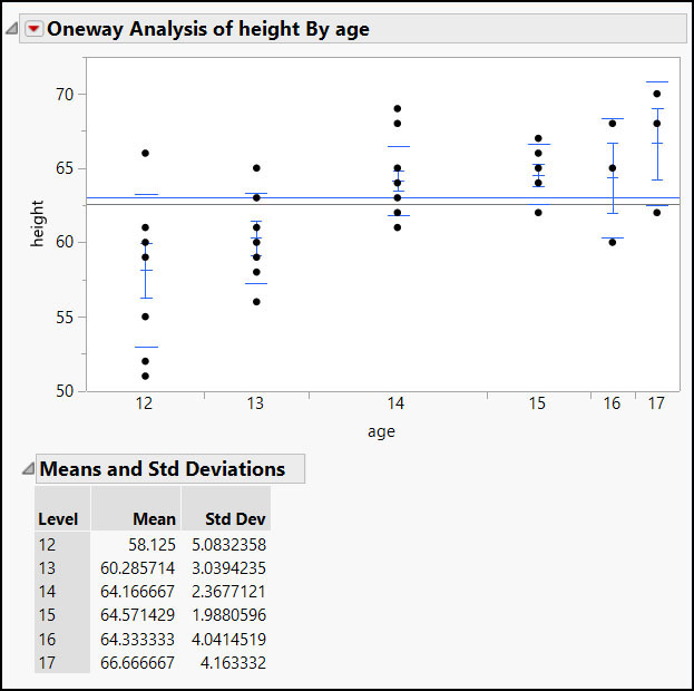
colsToHide << Visibility("Collapse" );
Figure 7.7 Oneway After Columns Are Hidden
What is an expression? In JMP, it is something that can be evaluated. It can be a combination of variables, constants, or even a collection of scripting commands linked by operators. Why is it important to a scripter? Because there are times when you want to wait to evaluate, or simply control when to evaluate, such as when a user must be prompted for a response that will be used to initialize a variable.
JSL provides expression-handling functions to facilitate this control. Eval() is used to evaluate arguments, whereas others, such as Expr() and Eval Expr(), are containers that control how their expression arguments are evaluated.
Everything within the argument of the Expr() function is considered an expression. The argument contents can be numeric or string literals, variables, arithmetic expressions, or a combination of any or all. These examples are all expressions:
Expr( 5 + 1 );
Expr( y = m * x + b );
Expr( "The weather is sunny" || "in Aspen." );
Expr( For (i = 1, i <= 5, i++, Print(i) ));
If you execute these in a script window, the results show the arguments for each Expr() function. No attempts were made to simplify the expressions or evaluate any variable.
The Eval() function evaluates the expression and returns the result. If we wrap all the preceding expressions in Eval(), we see these simplified results:
Eval( Expr( 5 + 1 ) );
m = 0.5; x = 2; b = 5; Eval( Expr( y = m * x + b ) );
Eval( Expr( "The weather is sunny " || "in Aspen.") );
Eval( Expr( For( i = 1, i <= 5, i++, Print( i ) ) ) );
//:*/
Eval( Expr( 5 + 1 ) );
/*:
6
//:*/
m = 0.5; x = 2; b = 5; Eval( Expr( y = m * x + b ) );
/*:
6
//:*/
Eval( Expr( "The weather is sunny " || "in Aspen." ) );
/*:
"The weather is sunny in Aspen."
//:*/
Eval( Expr( For( i = 1, i<= 5, i++, Print( i ) ) ) );
/*:
1
2
3
4
5
A good method to evaluate an expression within any expression is to use the Eval Expr() function. This function replaces each Expr() argument with its evaluated value.
The syntax is very simple. The given argument must be an expression:
Eval Expr( expr )
In this example, we want to create a bivariate plot using a Where statement, and the value to be used for the Where statement is stored in the selVar variable.
dt = Open( "$SAMPLE_DATA/Fitness.jmp" );
selVar = "M";
biv = dt << Bivariate( X( :MaxPulse ), Y( :RstPulse ), Where( :sex == selVar ) );
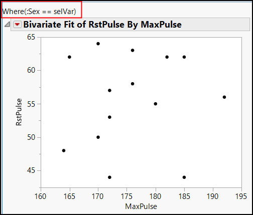
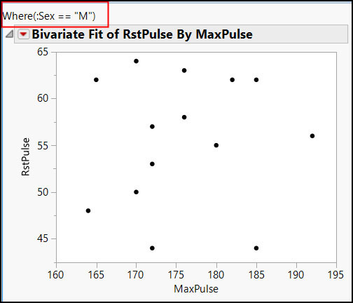
If we simply use Where (:sex == selVar), the graph appears to be correct, but the Where statement above the graph shows the variable name, not the variable value:
Figure 7.8 Bivariate Report without Using Expressions
Put the Bivariate command in an expression, and wrap the variable, selVar, in an Expr() function:
bivExpr = Expr(
    dt << Bivariate( X( :MaxPulse ), Y( :RstPulse ), Where( :sex == Expr( selVar ) ) )
);
Place the bivExpr as argument to Eval Expr():
EvalExpr( bivExpr )
If you execute this code, you will see in the log that the value of selVar has been inserted into the expression bivExpr:
Bivariate( X( :MaxPulse ), Y( :RstPulse ), Where( :sex == "M" ) )
In order to execute the expression, the Eval() function should encompass the Eval Expr() function:
biv = Eval( Eval Expr( bivExpr ) );
The complete code is as follows:
dt = Open( "$SAMPLE_DATA/Fitness.jmp");
selVar = "M";
bivExpr = Expr(
   dt<< Bivariate( X( :MaxPulse ), Y( :RstPulse ), Where( :sex == Expr( selVar ) ) )
);
biv = Eval( Eval Expr( bivExpr ) );
The desired results are achieved, as Figure 7.9 shows.
Figure 7.9 Bivariate Where Statement When Using Eval Expr()

Using Eval Expr() is also a favorite method when replacing variable values in a column formula. This example shows how to use it in a column formula, replacing a value at run time.
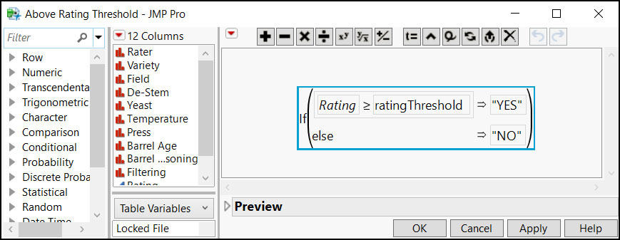
We have a table on wine data, including a ranking of each wine. A column with a formula is added to the table to show that if a wine has a rank above the threshold, then “YES” is assigned, and when the rank is below the threshold, then “NO” is assigned. The threshold, determined by the user, is initialized in the variable thresholdRank.
The problem is that if the following script is executed, the formula in the new column retains the variable ratingThreshold, which is not initialized and produces an error when the table is opened in a subsequent new session of JMP:
dt = Open( "$SAMPLE_DATA/Design Experiment/Wine Data.jmp" );

ratingThreshold = 10;

thresCol = dt << New Column( "Above Rating Threshold",
   "Character",
   "Nominal",
   Formula(If( :Rating >= ratingThreshold, "YES","NO" ) )
);
Figure 7.10 Formula Editor
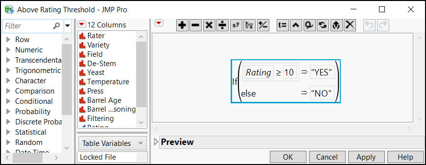
A better way to handle this is to use Eval Expr() to replace the variable with its evaluated value in the formula:
dt = Open( "$SAMPLE_DATA/Design Experiment/Wine Data.jmp" );

ratingThreshold = 10;

thresCol = Eval(
   Eval Expr(
        dt << New Column( "Above Rating Threshold",
           "character",
           "nominal",
            Formula( If( :Rating >= Expr( ratingThreshold ), "YES","NO" ) )
       )
   )
);
Figure 7.11 Formula after Using Eval Expr()
Sometimes you need to replace a value in an expression before it is evaluated. This happens frequently when you are creating the expression dynamically at run time. The Substitute() expression-handling function can replace parts of your expression with the stored argument.
Here is the syntax for this function:
Substitute( x, patternExpr1, replacementExpr1, …)
In the Eval Expr() example shown previously in this chapter (see Figure 7.8), we can instead use Substitute() to place the value of selVar into an expression containing the Bivariate command.
Here is the original script:
dt = Open( "$SAMPLE_DATA/Fitness.jmp" );
selVar = "M";
biv = dt << Bivariate( X( :MaxPulse ), Y( :RstPulse ), Where( :sex == selVar ) );
Create the Bivariate expression:
Expr(
   Bivariate( X( :MaxPulse ), Y( :RstPulse ), Where( :sex == choice ) )
)
The variable choice was inserted as a placeholder. Notice that the entire command is wrapped with the Expr() function.
Next, use the Bivariate expression as the first argument for the Substitute() function, and then add the second argument as the expression that will be replaced. The third argument is the variable value to be used as the replacement:
Substitute(
   Expr(
       Bivariate( X( :MaxPulse ), Y( :RstPulse ), Where( :sex == choice ) )
   ),
   Expr( choice ), selVar
)
If you execute the Substitute() function as is, you will see in the resulting log that the replacement has been made:
Bivariate( X( :MaxPulse ), Y( :RstPulse ), Where( :sex == "M" ) )
Substitute() has made the replacement in the expression, but to execute the expression, the Substitute() function must be wrapped in an Eval() function:
Eval(
   Substitute(
       Expr(
           Bivariate( X( :MaxPulse ), Y( :RstPulse ), where( :sex == choice ) )
       ),
       Expr( choice ), selVar
   )
)
The finished code looks like this, and produces the results shown in Figure 7.12.
dt = Open( "$SAMPLE_DATA/Fitness.jmp");

selVar = "M";

biv = Eval(
   Substitute(
       Expr(
           Bivariate( X( :MaxPulse ), Y( :RstPulse ), Where( :sex == choice ) )
       ),
       Expr( choice ), selVar
   )
);
Figure 7.12 Bivariate Report Using Expressions and the Substitute() Function
The Substitute() function is very handy. It can also be used if you need to replace multiple occurrences of the same variable within an expression. Please see its entry the Scripting Index for additional examples.
Finally, there are other helpful functions to investigate, such as Eval Insert(), Name Expr(), Parse(), and Eval List(). Search for these in the Scripting Index to learn how these functions can help you in your scripts.
You might have heard the saying that 80% of the work is done in 20% of the time. That is definitely true when it comes to writing a complex script. For many of us, it is fun to write a script that builds a neat interface and accomplishes an important task. That’s where creativity is most fulfilled, right? It is that last 20% of the work that ensures that all the details are taken care of that will prevent your script from breaking.
In the context of JMP scripts, the concept of defensive programming encompasses various types of condition handling to prevent exceptions. These strategies are used to make your script durable. Remember, not all errors are unexpected.
At the start of your script development, it is important to spend time considering possible situations and how they should be handled. For example, suppose your script prompts the user to open a data file. What if a text file was selected but you were expecting an Excel file? Or what if the user supplies fewer columns to your custom launch window than is necessary for the remainder of your script to run successfully? What if they just click Cancel? These are examples of conditions that you can easily handle in your script. The following are some things you can do to handle such situations:
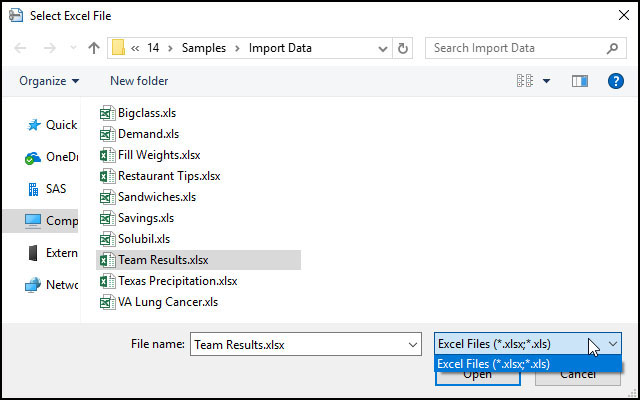
● Wrong File Type – The Pick File() function offers a filter list option, which limits the files shown in the dialog to those that are specified. If your script’s Open() function has options that are specific to a particular file type, such as Excel, you can specify only Excel file types in the filter list option. Here is an example that demonstrates the filter list:
excelFile = Pick File(
   "Select Excel File",      //Prompt message
   "$SAMPLE_IMPORT_DATA",   //Initial directory
   {"Excel Files|xlsx;xls"}, //Filter list (with Excel file types only)
   1,                       //Filter to show (if more than one filter)
   0,                       //File action: Open = 0, Save = 1
   "",                      //No file initially selected
   //"Multiple"              //Option to allow selection of >1 file
);
Figure 7.13 Pick File() Dialog
● Incorrect User Input – When you are building a script with custom dialogs, it is easy to focus on getting your code to work for the expected inputs. But you should also take care that the expected inputs are the only inputs allowed. Familiarizing yourself with the options available for the display boxes that make up your custom dialog helps you do just that.
In the following example script, we use a Col List Box to prompt the user to select a column:
nw = New Window( "Launch",
   <<Modal,
   V List Box( Align( "Right"),
          Panel Box( "Select columns to analyze",
                 Lineup Box( N Col( 3), Spacing( 5 ),
                        clbAll = Col List Box( Data Table( dt ), "All"),
                        Button Box( ">>",
                               clbGet = clbAll << Get Selected;
                               clbSelect<< Append( clbGet );
                        ),
                        clbSelect = Col List Box( )
                 )
          ),
          H List Box(
                 Button Box( "OK",
                        analyzeCols = clbSelect << Get Items;
                 ),
                 Button Box( "Cancel" )
          )
   )
);
Figure 7.14 Custom Launch Dialog
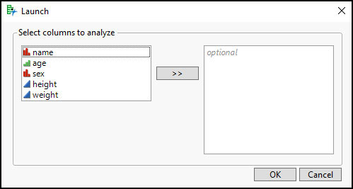
This dialog, though simple, looks okay. Little is done to ensure that the expected columns are selected. Notice the word optional in the box on the right? This means that columns of any data type can be selected, but no columns have to be selected, which is not likely what you want. So although your script would work perfectly for the expected inputs, you need to prevent any unexpected inputs.
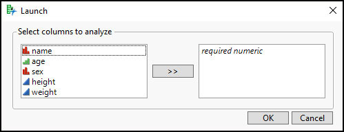
By reviewing the Col List Box entries in the Scripting Index and the JSL Syntax Reference, you will find optional arguments that enable you to control the number of columns that can be added, as well as the data type and modeling type, if desired. By adjusting the options in the Col List Box referenced by clbSelect, we can ensure that only one numeric column is selected.
clbSelect = Col List Box(
       Data Table( dt ),  //Optional data table reference
       "Numeric",        //Numeric columns only
       MinItems(1 ),     //At least one column required
       MaxItems(1 ),     //No more than one column accepted
       Nlines(5 )        //Number of lines to show
)
Now the box on the right shows the text required numeric, which provides a clear indication for the user that a numeric column should be selected.
Figure 7.15 Updated Custom Dialog
|
|
There are many more options to discover that would enable you to specify both data and modeling types, and more. So we definitely recommend that you review the options in the documentation. Also, be sure to check out chapter 9 for more examples of custom dialogs! |
● User Clicks Cancel – If the user were to click Cancel in the Pick File() dialog, the value in excelFile would be an empty string. If the "Multiple" option were used (commented out in the preceding example), then the value stored in excelFile would be an empty list. To ensure your script exits gracefully, you can add a check that stops the script when the value in excelFile is either an empty string or an empty list.
If( excelFile == "" | excelFile == {},        //Check for either
   Throw("User clicked Cancel." )
);
In this case, if either condition is true, the Throw() function is used to stop the script execution and to print a message in the log.
If the user were to click Cancel in the modal New Window, you would need to check the value of the nw reference. In this case, the value of nw would be {Button( -1 )}.
If( nw["Button"] == -1,
   Throw("User clicked Cancel." )
);
This script checks for the -1 value returned by the button. If the condition is true, the Throw() function is used again to stop the script execution and to print a message in the log.
● Differences in User Results – When you are scripting an analysis, it’s easy to assume that the results you see are exactly what another user will see when they run your script. Neglecting to consider that others might have different preference settings that could affect the results of your script is certainly an easy thing to do.
Consider the following example. The script opens a sample table and runs a Distribution on two columns.
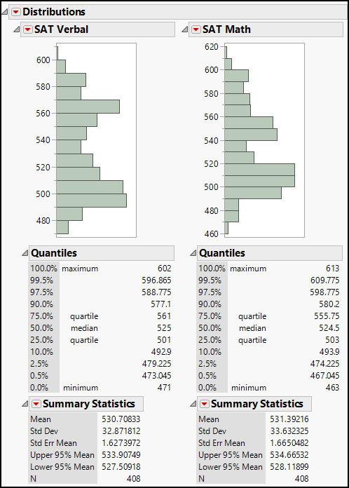
dt = Open( "$SAMPLE_DATASATByYear.jmp");

dist = dt << Distribution(
   Continuous Distribution( Column( :SAT Verbal ) ),
   Continuous Distribution( Column( :SAT Math ) )
);
The output when you run the script is as shown in Figure 7.16.
Figure 7.16 Expected Output

But when your colleague runs the same script, the result is as shown in Figure 7.17.
Figure 7.17 Output for Another User
So what happened? Because your script does not explicitly stack the output, the results for this colleague do not have the eye-pleasing layout that you intended. And it appears that your colleague has the Outlier Box Plots turned off in their preferences.
If the layout and options that you see are important to what you are trying to convey, then those options need to be explicitly accounted for in your script. For this example, you can ensure the output is stacked and the Outlier Box Plots are turned on by making the following hightlighted adjustments:
dist = dt << Distribution(
   Stack( 1 ),
   Continuous Distribution(
Column( :SAT Verbal ), Outlier Box Plot( 1 ) ),
   Continuous Distribution(
Column( :SAT Math ), Outlier Box Plot( 1 ) )
);
Now the script will generate the desired output regardless of the user’s preference settings. As we said, it is an easy mistake. It might have been that you turned on the Stack option in your Distribution platform preferences so long ago that you have forgotten that it is not the default. Or maybe it just never occurred to you that someone would turn off a default setting. The point here is that if it is important to your result, be sure it is included in your script.
With plenty of condition handling in the script, we hope you won’t have to deal with any exceptions. But sometimes there are problems with the logic in the script, or there is a situation that you just did not think of that causes an error. Shocking, right? But it does happen. So what are some other things you can do to limit the chances that your script will fail or otherwise behave inappropriately when something unexpected happens?
Catch and Escape Exceptions
The Try() function evaluates an expression supplied as the first argument. If that expression causes an error, an optional second argument is evaluated and then the remainder of the script is executed. Sounds a bit like a get out of jail free card, doesn’t it?
Sometimes, you might want the script to stop executing when an error is encountered. In that case, you would include a Throw() function in the second argument. Although Try() and Throw() are often used together, they can each be used alone. Let’s consider a situation where a Try()might be useful.
Suppose your script is designed to import data that might or might not contain a specific column. If you tried to reference a column that was not found in the data table, then your script would stop executing and in the log you would find an error. Depending on how you referenced the column, you might see errors such as Name Unresolved or Scoped data table access requires a data table column or variable or something similar.
So before your script continues, how can you find out if the column exists? In the following example, we just try a simple action to test if an error will be produced. If the evaluation returns an error, then we print a message to the log and add the desired column. After the Try() is complete, the script will continue to execute:
Try(
   dt:Calories from Fat << Get Name,
   Print("Adding Calories from Fat column");
   dt<< New Column( "Calories from Fat" );
);
Print( "Script continues..." );
Some of you might be thinking that there are other ways to check the existence of a column. And you are right. As with most things in JSL, there’s more than one way to accomplish this task. In the following example, we demonstrate that you can capture a list of column names and then check to see whether the name is included in the list.
colNames = dt << Get Column Names( "String");

If( !Contains( colNames, "Calories from Fat" ),
   Print("Adding Calories from Fat column");
   dt<< New Column( "Calories from Fat" );
);
Print("Script continues..." );
As you can see, it took a little bit more script to write, but it accomplishes the same task.
Test Your Script Thoroughly
Another saying you might have heard is that no software is fully tested until it gets into the hands of the users. That is so true. When you know what the script is supposed to do, it can be hard to think of ways to make it fail. We suggest that you have a second set of eyes to try out your script. Even ask them to try to break it. Very often, this will unveil conditions that you have not accounted for in your script.
As an added bonus, you will probably get some feedback. Whether that results in new requirements and ideas for a future version, or causes you to reconsider certain aspects of your approach, feedback is a good thing.
The key to being a good scripter is knowing how to put together all the concepts and methods discussed to this point. In the next section, we will show you how to accomplish various tasks using the concepts described in the first section of this book.