
Chapter 5
Digital systems 2 – Arduino input
This chapter continues the introductory guide to programming, where you will learn about the core instruction types of iteration and selection (for system input). Several practical examples are provided that build towards the final MIDI Drum Trigger project as a learning milestone within the book, so it is recommended to spend some time working through them carefully to become familiar with the concepts involved and how to apply them. As chapters 4 and 5 are not a substitute for a full programming course, the chapter begins with a brief recap on the previous chapter to reinforce the core concepts involved. The chapter will discuss arrays (groups of variables) and iteration (repeating instructions) as a means of working through large amounts of data quickly – the ability to process data is the most powerful aspect of any computer. Arrays are used as a means of extending data, allowing note sequence information to be stored in a single logical structure. The chapter also looks at the second instruction type (iteration) as a for loop to process each element of an array in sequence and output sound to a piezo loudspeaker using the Arduino tone() function. This process is then extended by including an external code library to send MIDI messages over USB to a digital audio workstation (DAW) running on a computer. By replacing the previous tone() function with MIDI messages, the Arduino can be used as a MIDI controller within a larger MIDI system.
At this point, you have learned how to use programming instructions to generate output from the Arduino, but the real value for audio electronics systems lies in using selection instructions to control outputs based on system inputs. This chapter will look at how the Arduino can receive and analyse input using selection instructions, which are introduced by example (they are arguably the most complex aspect of programming to learn). Digital inputs to the Arduino from push-button switches are then used as the conditions in a selection statement, to determine what MIDI information to output. In so doing, you will also learn about the three stages of testing needed when working with a full Arduino system:
1.Test the code – if the Arduino code is wrong, then the system cannot process information.
2.Test the board – if the circuit is wrong, then the system cannot receive inputs and create outputs.
3.Test the system – if the code and the board are functional, we must then test the full system.
Finally, you will learn how to analyse analogue input from a piezo sensor, as part of the final project to construct a MIDI drum trigger. The chapter builds towards a final project that uses piezoelectric sensors as inputs to an Arduino MIDI drum trigger – a fully functional project that you can connect to your own DAW to control a software drum machine that will accept MIDI data. At that point, you will have built your first full electronics system that takes input from a piezo sensor, processes it using the Arduino and outputs MIDI Note messages. This is a learning milestone in this book, which combines audio systems design, DC circuit analysis and Arduino C programming to produce a fully functional MIDI drum trigger system. If you have followed the text and examples correctly, you will complete this chapter with your first functional electronics system that has numerous possibilities for extension and augmentation into a more robust and flexible MIDI controller. More importantly, you will understand the concepts involved in designing and building such a system, which arguably equips you with the knowledge required to progress your learning in areas such as C programming – beyond the introduction provided in this book.
5.1 Programming recap
The previous chapter introduced the three core programming instruction types:
We learned that all sequence instructions must be terminated with a semicolon (;) to prevent the compiler from seeing the next instruction as part of the previous – the semicolon is the fundamental means of punctuation in C/C++ programming. The chapter also covered functions – structures that encapsulate code (Figure 5.1).

Functions were used in the examples to reduce and reuse code, allowing us to add PWM output to a piezo loudspeaker relatively quickly to our existing blinking LED code. In so doing, we also made use of constants and variable – named storage locations in memory (Figure 5.2).

In the previous chapter, we learned that functions group code instructions in a single uniquely named structure. Now we can extend our learning to include arrays – uniquely named data structures that group variables in a single referenced location in memory.
5.2 Data structures and iteration – arrays and loops
The previous chapter introduced variables, which are named memory locations, that can be used to hold a reference to a value that may change. The natural-language comparison was made with variables as nouns, that instructions (verbs) can process – you cannot have a verb without a noun. This thinking can now be extended to group related variables together, making them much more easily accessible within a single structure known as an array (Figure 5.3).

In this diagram, an array is initialized by declaring the type of the elements (variables) in the array – the examples use integer types. We initialize an array using a sequence instruction, and so this requires a semicolon to terminate it correctly. We then assign (=) the value for each variable by separating them with commas within a set of braces – you may have heard of comma-separated values (CSV). Notice that each array begins from index zero (0) – this is a crucial point to remember as we declare the array with the actual number of elements:
When declaring a new array, we specify the number of elements in the array inside the square brackets. We can then access a specific array element by passing its index into the square brackets:
Now we know the basics of how to initialize and access an array:
1.To initialize, define the type and pass the array length into the square brackets: byte exampleArray[4].
2.To access, pass the element index into the square brackets: exampleArray[2].
Arrays can be difficult to learn in abstract, but for the purposes of this book will be kept as straightforward as possible. It is important to remember that because we count array elements from index zero, the last element is always one lower than the length of the array. Arrays allow us to group associated data together, and as we expand our code this will become more necessary. Thus this chapter will not go into extensive discussion of arrays, but you will use them to structure your code more effectively in later examples. To do this, we now need to learn how to use the second core instruction type – iteration.
We can repeat certain instructions in our code by defining them within a for loop that iterates a specific number of times. For loops require start and end values, and also the increment (step size) value used to count between them (Figure 5.4).

The diagram shows how a for loop uses a count variable to determine how often to iterate the instructions within the loop. The count requires a start and end value, alongside a step value that defines how much to increment the count by each time (this is usually 1):
In the listing, a variable called loopCounter is declared to control a for loop (you will encounter many examples that use single letters, but descriptive names will be used in this book). When the loop is set up inside the brackets, three sequence statements (terminated by a semicolon) are declared to do the following:
1.Assign the value 0 to loopCounter – this defines the start of the loop.
2.Evaluate the result of the expression loopCounter < 4 – this defines the end of the loop.
3.Increment the loopCounter variable by 1 (loopCounter ++) – this defines the step of the loop.
Expressions (e.g. x<y, a>b) will be discussed later in the chapter when we learn about conditions, but for now we can see that a loop starting at 0 and stopping at less than 4 (i.e. 3) will iterate 4 times. Any instructions inside the braces will execute each time the loop iterates, and we can specifically control how often this happens when we set the loop up. Loops are very powerful coding instructions that are used frequently, particularly in conjunction with arrays to allow all elements to be processed in the same way. To use a for loop with an array, we need to know the array length so we can iterate through all of its elements (Figure 5.5).

This leads to a code structure that requires both the array and its length to be defined in order to iterate through it using a for loop:
The listing above defines a constant called arrayLength that is used to create an array of five elements – don’t forget arrays begin at index 0. We can then initialize our array by stating its type (byte) and passing arrayLength inside the square brackets. Next, we use a for loop that counts between 0 and arrayLength in increments of 1 (++) – don’t forget arrays begin at index 0, so we will actually be counting from 0 to arrayLength−1 (4). Inside the loop, we access each array element by passing the loop counter into the array square brackets as the index required. We can then use the value stored at this index to setup a digital pin for output using the pinMode() function.
Take some time to read over the last code listing, as the combination of data and iteration is very useful for common coding tasks like pin configuration and digital output. In the previous chapter example project we learned how to declare constants corresponding to specific Arduino pins, how to initialize those pins for output and then how to use a function to send digital signals (including PWM) to them to light LEDs and emit sound from a piezo loudspeaker. A smaller version of this project can show how iteration can be used with an array to significantly streamline this code – whilst also ensuring that fewer mistakes are made due to manual repetition of the instructions.
5.3 Example 1 – tone array output
In this example, a stripped-down version of the final project from the previous chapter is used that does not require LEDs, to reduce the overall build time involved. In the chapter 4 project example, three tones (C4, D4, E4) were output in a simple sequence using the flashToneOutput() function that combined LED output with tone() function calls to send PWM output to the piezo loudspeaker. In this example, we will extend this tone sequence to output 16 tones in a much longer musical pattern sequence. The instructions for this longer tone sequence could be coded manually, but this would take significantly more time and would also be prone to errors (e.g. due to the fatigue of repetition). Instead, we will use an array to hold our note frequency values and then iterate through them using a for loop to output this much longer melody to the piezo loudspeaker. This demonstrates the power of arrays when combined with for loops as a means of working with larger amounts of data (Figure 5.6).

The system shown in Figure 5.6 is fairly straightforward in electronic terms, consisting of a single PWM digital output that is used to drive a piezo loudspeaker. The setup() function initializes pin 10 for digital output using pinMode(), whilst loop() makes a call to the soundOutputPin() function that processes the array. The setup() and loop() functions are short, as the majority of the processing work is carried out by soundOutputPin(). At first glance, the function soundOutputPin() can appear a little redundant, as we could simply execute these instructions in loop(). Though this is appears to be the simpler option, we are actually using the function call to soundOutputPin() to keep the loop() function simple and easier to read. In addition, it is good practice to avoid calling a function every time loop() executes to keep our system processes to a minimum (thus saving battery life and reducing needless instruction executions).
In addition, parameters are still being passed into the soundOutputPin() function for both the output pin (10) and also the toneArray(), even though these could simply be stated within the function itself to make the call simpler. This is done to reinforce the concept of passing parameters within function calls, which also has the added effect of making us fully consider the data used by the processes involved when declaring the function itself – we could call a function that uses lots of different data, but we would be less likely to track that data from the call to that function. Although the previous chapter did not go into extensive detail on functions, the aim is still to present examples that show how best to use them to control electronics systems.
From this system diagram shown above, we can now build a Tinkercad circuit layout based on the following example schematic (Figure 5.7).

This schematic is fairly straightforward, but if you are unsure of how a digital output pin from the Arduino can generate PWM output to drive a piezo loudspeaker then it is recommended to look over the previous chapter again to refresh your memory of Arduino output. It should also be recalled that the 150Ω resistor is added in series with the loudspeaker to limit the current flowing through the circuit. The Arduino can only output a maximum of 40mA on a single pin so we want to avoid burning out either the Arduino and/or the loudspeaker. You should also remember that we have gone slightly higher than needed (125Ω) to 150Ω (
![]() ) to allow us to use the same resistors as in our other examples to keep our circuit costs down (and that 220Ω resistors can be used instead). This schematic can now be translated into an Arduino breadboard layout (Figure 5.8).
) to allow us to use the same resistors as in our other examples to keep our circuit costs down (and that 220Ω resistors can be used instead). This schematic can now be translated into an Arduino breadboard layout (Figure 5.8).

This breadboard layout is fairly straightforward, and as previously noted is a stripped-down version of the chapter 4 example project. As with the circuit layout in that chapter, it is again noted that in practice you may need to rearrange the pin layouts based on the specific piezo loudspeaker you have, as the Tinkercad component provided is significantly bigger than many others available. The connection instructions for this circuit are as follows:
1.Add a 150Ω resistor between pins [i1–i5].
2.Add piezo loudspeaker between pins [h5–10].
3.Add a connector to the negative (ground) rail [i10–GND].
4.Add a connector between the negative (ground) rail (near column 11) and the Arduino top left GND pin.
5.Add a connector between Arduino digital pin 10 and breadboard pin j1 [AD10–j1].
From the system code process diagram, we know that we will have to declare an array named toneArray() to hold our note frequencies, a constant to define the output pin (10) alongside three functions in our code. Setup() and loop() will be kept as simple as possible, with the majority of the instructions being contained within the soundOutputPin() function:
The listing above shows the complete code for the example – you can copy/paste this into the Tinkercad simulator, or upload it directly onto an Arduino Uno board using the Arduino IDE. An array is declared containing 16 note frequencies with toneArray[toneArrayLength], and then the soundOutputPin()function is used to iterate through this array to generate PWM output at the frequencies specified in the array using the tone(pinNumber, toneSequence[loopCounter])function. The toneArrayLength constant is used to define the length of our array and also the length of our loop, to ensure we iterate through all the elements.
If the circuit has been built correctly, you should now hear a looping sequence of tones from the piezo loudspeaker as output. To save time, an actual build of this circuit will not be provided as the next example on Arduino MIDI output will require a physical circuit to be built for full system testing – this will require you to follow a series of tests that will help translate a simulation to an actual circuit that cannot be fully simulated by Tinkercad. In programming terms, you have now reached an important stage in our understanding of code processes. You can now declare and call a function that iterates through an array of variables to generate Arduino output. In the next section, we will consider how to extend this circuit by replacing the piezo loudspeaker with a simple MIDI hardware interface – allowing us to use our Arduino to generate a MIDI sequence as output.
5.4 Working with external libraries – serial MIDI output
Chapter 2 introduced the Musical Instrument Digital Interface (MIDI) protocol, which uses a 5-pin DIN (Deutsches Institut für Normung) connector to establish communication between devices (Figure 5.9).

In Figure 5.9, two triangles are shown that represent operational amplifiers (these will be discussed in more detail in chapter 7). The rest of the schematic uses three pins of the 5-pin DIN connector, with pins 4 and 5 having current-limiting resistors (the MIDI specification defines 220Ω) for both signal pin 5 and pin 4 (+5V). The signal from the Universal Asynchronous Receiver Transmitter (UART) is a serial communication of binary bits grouped into bytes, based on the MIDI message format (Figure 5.10).
|
Status |
Channel |
Data 1 |
Data 2 |
||||||||||||||||||||
Note On (9) |
1 (binary 0) |
Middle C (60) |
Velocity (100) |
||||||||||||||||||||
1 |
0 |
0 |
1 |
0 |
0 |
0 |
0 |
0 |
0 |
1 |
1 |
1 |
1 |
0 |
0 |
0 |
1 |
1 |
0 |
0 |
1 |
0 |
0 |
The table details a Note On message, which is a common 3-byte MIDI message sent in a serial (sequential) format. A Note On message is configured as follows:
1.Status – four status bits define the message type, where Note On is 1001, or decimal 9 (Note Off is 1000, decimal 8).
2.Channel – four bits that define the MIDI channel (1–16) that the message is intended for (counting from binary 0).
3.First data byte – defining a 7 bit note number from C-2(0) to G8(127). On an 88-key piano A0 (21) to C8 is (108).
4.Second data byte – defining the velocity of the note (from 0 to 127).
MIDI messages are examples of discrete signals (more commonly known as digital signals), which were previously introduced in chapter 2 (section 2.2). A discrete signal can either be 0 (low) or 1 (high), where these two values are represented by distinct voltage levels within a digital electronic circuit (Figure 5.11).

Thus MIDI is a digital system that sends data as a combination of binary bits that are represented by voltage levels, where these bits are grouped into 8-bit bytes for processing. An important thing to note is that all MIDI values are in binary, so they are counted starting from 0. This means that MIDI channel 1 is binary 0, which is important to know as all MIDI software (and hardware) interfaces count from decimal 1 to 16! In contrast, a Note Off message only requires 2 bytes (to specify the status/channel and note number) but instead most modern devices use a second Note On message with zero velocity as part of a technique known as running status. Running status assumes that the first MIDI message contains the status/channel required, and unless another status byte is received then every subsequent first or second data bytes will be assumed as being another Note On message for that channel. This also explains why MIDI data bytes (e.g. notes and velocities) have a 7-bit range (0–127), because the most significant bit (MSB) of the message must always be zero to avoid it being seen as a possible status byte (Figure 5.12).

In this example, the same note (C4) is played three times, once with velocity 100 (1100100), then with a louder velocity of 125 (1111101) and then finally with velocity 0 (which is effectively a Note Off). By streamlining the data sent, MIDI can be much more responsive to note timings because it does not have to send status messages with each one. Now we understand a little more about MIDI messages, we can learn how the Arduino can be configured to send serial data on a digital output pin in the form of MIDI messages. In Figure 5.9, it was shown that the MIDI UART runs at 31250 baud, where baud is a unit of transmission speed that defines the number of bits per second that can be can transmitted by MIDI. Our Arduino also has a built-in UART, which can be set up to output on a digital pin at this rate (Figure 5.13).

In this diagram, a multi-stage system has been defined that combines an Arduino MIDI output circuit with a computer sequencer and/or synthesizer that can receive MIDI output. This is the first system that must also model its outputs as inputs to another system, so you may want to revisit chapter 2 (particularly Figures 2.4 and 2.7) to look over system boundaries and partitioning again. In the system above, a boundary is defined between the MIDI output connector and another MIDI system that may comprise any number of MIDI-compatible devices. This is one of the most powerful aspects of MIDI, in that any device that conforms to the MIDI specification can be connected to another. The MIDI sequence player circuit will form part of a larger MIDI system, which is partitioned to focus on the sequence player in terms of code and electronic components. When these elements are tested, they will also need to be combined within the full system to ensure everything is functional.
The Arduino UART can output serial data on digital pin 0 and receive it on pin 1 by default, but this connection must be used carefully on the Arduino Uno (or any ATMega328P board), as these pins are also reserved for serial communication with a computer running the Arduino IDE. This is why the system diagram stipulates pin 5 for output (see below). To understand how to program the Arduino UART to generate serial output, we can begin by using a single call to the Arduino Serial library:
In the listing above, a core Arduino library called Serial is used that will handle all serial port communications. The Serial library contains a list of functions that will configure and output serial data – these are the begin() and write() functions used in the listing above. To access a Serial library function, we must use the Serial object with a dot accessor to call it as shown above – Serial.begin(), Serial.write(). You have actually been doing this already with core Arduino functions like pinMode() and digitalWrite(), the only difference is the compiler already knows they are part of the core Arduino library and so doesn’t require you to state this object when you call them. Objects will not be discussed in detail as they are beyond the scope of these introductory chapters, but it can help to think of them as groups of functions and data.
The baud rate listed above is a common rate for boards like the Arduino, but it is not sufficient for MIDI, which requires 31250 baud. The begin() function call could be set to a higher rate, but there is also another issue that must be addressed – the pin conflict with USB. As noted in Figure 5.13, the Arduino Uno uses digital pins 0 and 1 for serial communication over USB, so these pins cannot be used for any other purpose while the Arduino is connected to a computer running the Arduino IDE. A workflow could be implemented where the board is unplugged before running any serial output, but this has the potential to confuse things when you are learning and even damage the Arduino by not disconnecting an output pin or running the code with the USB still connected. Instead, another Arduino library called SoftwareSerial can be used that can write serial data to other digital pins. To do this, we must include its library of functions at the beginning of the code using the following statement:
In the listing, the library is included so its functions can be used by calling a constructor function to create a new SoftwareSerial object called SerialMidi that receives on pin 4, and transmits on pin 5. Calling object functions is a more advanced programming technique, so while the terms used are explained for clarity, it is recommended that when beginning to learn both audio electronics and Arduino programming (at the same time!) it is better to know how to use objects rather than fully understand how to build them – there are many object-oriented programming (OOP) resources available should you wish to extend your knowledge after completing this book.
For now, the serial port is initialized (at standard 9600 baud) and then the SerialMidi software object is configured at 31250 baud. With the ports configured, a MIDI message can now be sent by the SerialMIDI object using its write() function:
MIDI messages are sequential, so by writing each byte in turn a serial MIDI message is output to digital pin 9. The first byte is the status byte (status/channel), which for a Note On message (1001) on MIDI channel 1 (0000) gives a binary value 10010000. In the code listing, this is converted into hexadecimal (base 16 numbers) to make it easier to program the value than by typing it in binary (where a mistake could easily be made in the digits). Although hex may seem complex, it is very common in computing – if you’ve ever used a computer graphics program then you will be familiar with hex colour codes. This book will not cover the hexadecimal number system, but as with objects we can make use of it to send a Note On channel 1 status byte (channel 2 would be 0x91, channel 3 0x93 etc).
5.5 Example 2 – MIDI sequence player
This example combines the array-processing code from example 1 with MIDI output to create a MIDI sequence player. The main addition to the previous system is the use of the SoftwareSerial library to create an object that can output serial data to our MIDI connector. An array can then be used to iterate through a sequence of MIDI note numbers and output them on digital pin 9 (Figure 5.14).

The system in Figure 5.14 is very similar to example 1, with the main difference being the replacement of tone() function calls with write() function calls to a SoftwareSerial object. You will also note that the system from Figure 5.13 is partitioned to exclude the overall MIDI system that could be connected to the output of our Arduino circuit. This was done to focus coding development on the MIDI sequence player circuit, but the example will revert to the larger system again later for testing. The schematic for this system uses an Arduino digital output pin connected to the standard MIDI out schematic from Figure 5.9 (Figure 5.15).

The schematic shows digital pin 9 on the Arduino connected to pin 5 on a 5-pin DIN connector, with a current-limiting resistor being added to conform to the MIDI hardware interface specification shown in Figure 5.9. In addition, the 5V Arduino power pin is connected to pin 4 (also with current-limiting resistor) and pin 2 is connected to ground (GND) – this is a standard MIDI Out interface that is now interoperable with other MIDI equipment.
This circuit cannot be fully simulated in Tinkercad, as MIDI communication is beyond the scope of the tool – it does not extend to a communication technology like MIDI, nor provide any DIN connections. Tinkercad does provide a useful list of standard electronics components that are aligned to the most common uses of the Arduino, and we have used the LED and piezo loudspeaker actuator outputs provided until this point. Now we are beginning to move outside the scope of this tool and so will have to plan simulation and testing in different ways, to ensure that the simulator can still be used where possible. In this project, the code can still be checked to ensure it is compiling and executing correctly by tracking the output it generates. To do this, we can use the Serial Monitor window provided in Tinkercad (at the bottom of the coding editor) to print out values generated by the code. Whilst the SoftwareSerial object cannot be accessed for MIDI output, the print() and println() functions of the core Serial object can be used to output the MIDI status and data bytes to the Serial Monitor window (Figure 5.16).

This diagram shows how Tinkercad can be used to trace a simulation of the data output, which allows the project code to be tested to ensure it will output the correct values before we connect our MIDI interface circuit. You can look at the Serial Monitor window to see if the data has been generated correctly, but you must remember to click the Clear button at the bottom of the Serial Monitor to ensure the data is tracing from the beginning of the current simulation (otherwise the monitor will simply add it to the previous output).
With code output now traceable, testing can be planned to reduce the scope of any errors we may encounter. This is a useful process when working with microcontrollers, as we will always be combining code debugging, electronic schematic and breadboard layout issues and then finally checking that everything is physically built correctly! Sanity checks have been added during previous project builds (e.g. build stages) but now we will make a more focussed delineation between what can be tested by simulation and what must be physically tested:
1.Test the code – if the data is not correct, then the circuit will not function. Tinkercad can be used for this stage of the project.
2.Test the board – the circuit layout should reflect the schematic, to ensure all components are connected as required. There will be no output if we have not configured our layout properly, even if the code is functional.
3.Test the system – the outputs of the circuit should behave as required within the broader design of the system involved. When streaming binary data to a MIDI interface we will need to have a wider MIDI system to test this data.
These three testing stages can be used to check the entire project, to avoid making an error in one area that compounds others. For example, if there is a coding error that outputs the wrong data (or none at all) then there is no point in connecting the breadboard circuit. Similarly, if the code is tracing out as required, we know that either the serial communication is not configured properly or the breadboard layout is wrong – this can be tested with a simple output (like an LED) to quickly check for connection issues. If both of these stages are functional, the wider MIDI system can be checked with another known device to ensure it is capable of receiving and responding to messages on the specified channel.
The first testing stage involves the code needed to generate MIDI output, which will iterate through an array of MIDI note values to output them as serial MIDI data through a SoftwareSerial object on digital pin 9. The code from example 1 will be used as the basis for the MIDI output project, where the array-processing code has been moved into a dedicated function both to allow it to be tested separately and also to keep loop() simple. Now, this function can be reworked to output MIDI data to the SoftwareSerial object using the note values stored in the array. We can also use our Serial object to print the same data to the Serial Monitor, to ensure that we are building the structure of each MIDI note (and the sequence) correctly:
In the listing, the SoftwareSerial library is included using #include <SoftwareSerial.h> to allow serial communication to be sent on digital pins other than 0 and 1 (which are used by the Arduino IDE to upload the code over USB). The SoftwareSerial object SoftwareSerial SerialMIDI(4, 5) was then set up to handle communications on pins 4 (Rx) and 5 (Tx). An array of integers was declared to hold the MIDI note values int noteArray[noteArrayLength], which uses a constant noteArrayLength for the length of the array. Notice that as long as they are separated by commas, the array values can be declared across lines in the code – languages like C will continue to read the text after an array comma as being part of the array, so the declaration can be split to make it easier to read.
In setup(), the pinMode() calls from the previous examples are replaced to configure output pins with two begin() calls to start the Serial and SoftwareSerial SerialMIDI objects – you cannot run SoftwareSerial without the Serial object, and the Serial object can also be used to print data to the Serial Monitor for checking in the code tests below. The Serial object is configured to run at 9600 baud (which is a common value), while the SoftwareSerial object is set to 31250 baud for MIDI communication.
A call is then made in loop() to the midiOutput function – passing in the noteArray of MIDI note values and its length. The function iterates through midiSequence [] to access each value in noteArray (this array is passed in through the function call to midiOutput()). These values are then written to the SoftwareSerial object using SerialMIDI.write, which writes a status byte (0x90) and then a velocity data byte (100)after the note value to complete the Note On message (see Figure 5.10 for a Note On message example of middle C4 at velocity 100). The Serial object is then used to output the same data to the Serial Monitor, allowing us to check everything is correct. The function can then be tested in two steps: the first step checks the notes from the array by commenting out the print() calls for status and velocity, the second step checks the entire MIDI Note On messages by removing the comments and running all of the code:
If both code tests run correctly, you should see a list of note numbers that contain the array values for step 1 and then a list of full MIDI Note On messages for step 2 (Figure 5.17).

If code testing does not create both of these outputs, you must debug the code listing before continuing on to testing the board. Some simple debugging steps were introduced in the example project at the end of the previous chapter, but the first step is to check that you have performed the copy/paste of the previous code listing correctly – particularly because the listing now spans two pages in the book, it may be possible that a character was omitted.
With the code tested, we can move on to stage 2 of testing – test the board. Full MIDI output cannot be simulated on a breadboard circuit within Tinkercad, so full testing of the board is not possible without a physical circuit. The output of the SoftwareSerial object can be tested by using a resistor/LED loop as a visual validator of digital output on pin 5. In section 4.9 of the last chapter, the basics of pulse width modulation (PWM) were discussed, where a square wave can be output from a digital pin with a varying-length duty cycle to create an average voltage as a result. In this case, we can exploit the fact that serial binary communication is effectively no different than PWM output – the only difference is the shape of the wave (Figure 5.18).

In this diagram, the data for a typical MIDI Note On message (C4, velocity 100) is shown as a series of binary 1 (5V) and 0 (GND) output values. If considered as a PWM output, this data equates to a 37.5% duty cycle as there are a total of 9 binary 1 bits in a 24 bit message (
![]() ). For a 5V digital output from the Arduino, this gives an average output voltage of 5 × 0.375 = 1.875V, which provides enough current (
). For a 5V digital output from the Arduino, this gives an average output voltage of 5 × 0.375 = 1.875V, which provides enough current (
![]() ) to power the resistor/LED combination used in the circuits thus far (though the LED will be dimmer than in those circuits). This means the SoftwareSerial object output can be connected via digital pin 5 to a simple resistor/LED series loop to test whether it lights up (Figure 5.19).
) to power the resistor/LED combination used in the circuits thus far (though the LED will be dimmer than in those circuits). This means the SoftwareSerial object output can be connected via digital pin 5 to a simple resistor/LED series loop to test whether it lights up (Figure 5.19).

The circuit in the diagram in Figure 5.19 can be used as a (crude) digital signal tester – if the LED lights up then binary data is being sent by the SoftwareSerial object to digital output pin 9. By quickly testing the Arduino output connection to the board in this way, we can check the final piece of the code is functional without leaving the Tinkercad simulator. Although this project has now reached the limits of Tinkercad (the following chapters will use LTspice for AC circuit simulation), it has nevertheless been a very powerful and versatile addition to the development process for Arduino control circuits.
Having verified that the code generates a series of MIDI Note On messages for serial output on Arduino digital pin 9, the next step is to build the full circuit needed for MIDI connectivity – based on the schematic shown in Figure 5.15. Tinkercad can provide a breadboard layout for the circuit as a reference for this project, though the actual circuit can only be tested by building it on breadboard. In the diagram below, a mock-up of a generic component to represent a 5-pin DIN connector is provided as a reference for where such a component will be connected in the actual circuit (Figure 5.20).

In the diagram, the layout for a standard MIDI output interface based on the Arduino is shown. The Arduino provides +5V and GND connections for pins 4 and 2 (respectively) of the MIDI DIN connector, alongside a serial connection from digital pin 9 to pin 5 of the DIN that carries MIDI messages output by our code. This circuit can also be quickly modified for connectivity testing by placing an LED on pins [f15–f16] and connecting it to GND (right-hand diagram). If pin 5 of the MIDI connector is then disconnected (by removing breadboard connection j5) this effectively becomes the same serial communication test circuit as shown in Figure 5.19. This circuit can be used to test the SoftwareSerial code and then also test the board to ensure that MIDI messages are being sent to the MIDI DIN connector. Having said this, it cannot be verified that these MIDI messages are correctly structured until they are tested within the wider MIDI system introduced in Figure 5.13. To test this system, we must now build the actual circuit and connect it to a suitable MIDI interface that is capable of receiving (and responding to) MIDI data.
Project steps
For this project, you will need: 1. Arduino Uno board 2. One small breadboard (30 rows) 3. 1 × LED (for the test circuit) 4. 3 × 220Ω resistors 5. 1 × MIDI OUT connector (and MIDI cable to connect to a MIDI system) 6. 3 × connector cables and 7 × connector wires |
|
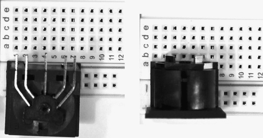
Add a 5-pin DIN MIDI Connector between pins [a1–a7]. The connector has a total of five pins (left-hand image), where the outer pins [a1] and [a7] are MIDI pins 1 and 3 (not used). MIDI pin 5 and MIDI pin 4 are extruded from the MIDI connector, this means that MIDI pin 5 is connected to [b2] and MIDI pin 4 is connected to pin [b6]. MIDI pin 2 is connected to pin [a4]. |
|
1. Add a 220Ω resistor between pins [g1–g5]. 2. Add a 220Ω resistor between pins [g6–g10]. 3. Add a connecting wire from breadboard pin j4 to the negative (ground) rail [j4–GND]. 4. Add a connecting wire from breadboard pin j10 to the negative (ground) rail [j10–GND]. 5. Add a connecting wire between pins [f1–e2] – this is the MIDI DIN pin 5 connection. 6. Add a connecting wire between pins [f4–e4] – this is the MIDI DIN pin 2 connection. 7. Add a connecting wire between pins [f6–e6] – this is the MIDI DIN pin 4 connection. |
|
1. Add a connector from Arduino digital pin 5 to breadboard pin h5 [AD5-h5] – this is the MIDI OUT connection. 2. Add a connector from the negative (ground) rail to Arduino GND pin [ADGND–GND]. 3. Add a connector from the positive rail to Arduino +5V pin [AD5V–V+]. |
|
For the LED test circuit: 1. Add a 220Ω resistor between pins [g11–g15]. 2. Add an LED – anode pin (f15) to cathode (f16). 3. Add a connector to the negative (ground) rail [j16–GND]. 4. Connect the Arduino digital pin 5 connector to pin f11 (not shown). |
|
1. Launch the Arduino IDE and create a new sketch called chp5_Example2. Copy/paste the full code listing for this project into the editor window. 2. Click the tick box in the top left of the editor to compile the sketch; if there are no errors you will get a ‘Done Compiling’ Message above the debug window. 3. After compiling, click the upload button (right arrow next to the tick box) to load the code over USB onto your Arduino. |
|
If this process has completed successfully, we can use the LED test circuit to check for serial MIDI output on digital pin 5.
|
|
Using whatever MIDI equipment you have available (either synthesizer or computer MIDI interface) connect a MIDI cable between the Arduino DIN socket and this system. Configure the system to receive MIDI data on channel 1. If the system functions correctly, you should now hear a tone sequence being output by the synthesizer in the MIDI system.
|
|


If everything has been built and tested correctly, you should now have a MIDI sequence player running on your Arduino that controls a MIDI-enabled synthesis device configured to respond on MIDI channel 1. Although the tone sequence will quickly become tedious to listen to (!), this represents a significant milestone in your learning, as you have now constructed a full MIDI output interface that can control another MIDI system to create sound output. In the following sections, this interface will be extended to respond to sensor input, first from switches (to learn about selection instructions) and then with a piezo sensor that acts as a drum trigger.
5.6 Conditions and digital input
At this point, a lot of programming concepts have been covered in a short space of time. The introductory programming chapters have discussed variables and sequence instructions, then looked at arrays (groups of variables) and functions (groups of instructions). This chapter introduced iteration as a means of processing the values in an array, leading to the MIDI sequence player example in the previous section. Now, we will look at the third (and arguably most complex) instruction type – selection. Selection instructions are essential to many areas of computing, but for this book they are primarily used to evaluate sensor input to a system. A selection instruction makes a choice based on a condition, where the condition is evaluated to be either true or false (Figure 5.21).

In computer programming, Boolean algebra is used to evaluate the logic of a condition to arrive at an outcome that is either true or false. Boolean algebra was first proposed by George Boole in 1854, and it has since been extended to become the foundation of all computer logic. The basic structure of a selection statement reflects this logic:
The code listing above shows the core structure that must be used in order to execute a selection statement – if/true else/false. The conditional true/false is used because they are the logical opposite of one another, but in practice it is more likely to use the distinction of digital HIGH/LOW on the Arduino as these can easily be mapped to the different voltage levels of +5V (HIGH) and 0V (LOW) in a circuit. Note that a pair of braces is used for each outcome of the condition, with a total of four (alongside two brackets to hold the condition) being required. This is an important point to remember before studying examples of selection instructions, as Boolean algebra can often become very confusing. When logical operators are combined with these extra syntactic elements of brackets and braces it becomes very easy to make mistakes with selection instructions, so it is recommended to return to the listing above if you become confused or frustrated with conditional logic.
Working from the basic structure of a selection instruction, the next step is to learn how to define the condition it will evaluate. This book provides an introduction to programming (it does not go into logical operators in depth), and it can be argued that understanding conditions is one of the most difficult aspects of programming to learn. The approach will be to keep the condition simple, to avoid some of the more confusing arithmetic and logical operators that are often used in coding tutorials and examples. This is done to provide an introduction, which can be extended over time to include more complex logic to model system input for human interaction with sensors.
A condition is any arithmetic or logical statement that can be evaluated as being either true or false. Conditions are thus constrained in their options, as the following examples show:
The above examples are deliberately simple, but already highlight the limitations of simple conditional logic. The definition of rain is seasonal, geographical and is rarely as simple as on/off. Similarly, tiredness is a complex combination of mental and physical fatigue alongside other emotional and motivational factors. These examples highlight the complexity of modelling human interactions – what initially appears to be a simple coding task can rapidly become a philosophical discussion – complexity cannot easily be modelled with simple logical outcomes. For this reason, the conditions in this book use switches as system inputs that function as on/off values. Although this makes teaching system inputs much simpler, real-world circuits will often be much more nuanced. Chapter 2 (section 2.5) introduced the simplest form of sensor input – the push-button switch. Now this switch operation can be used in a selection statement to define its condition (Figure 5.22).

The diagram defines the digital states HIGH (+5V) and LOW (0V) as being the two possible outcomes of the condition of a push-button switch (Arduino digital output was discussed in chapter 4 sections 4.2 and 4.3). This is where conditions are both simple and powerful; by working with digital signals (HIGH/LOW) as inputs they can easily be used in coding processes. For this condition, a +5V source can be connected to the switch and then the Arduino digitalRead() function can be used to determine the output value of the switch. If the switch is closed, then +5V (HIGH) will be present on both pins and the condition will be evaluated as true – when the switch is open, the pin will be seen as 0V (GND). In practice, an additional step is needed to ensure that the signal on the output pin will be 0V (LOW) when the switch is open, by adding a pull-down resistor to ensure the pin will always go to GND (Figure 5.23).

The explanation for pull-down resistors can become complex, as the concept of defining LOW (0V) and HIGH (+5V) voltage levels has practical constraints relating to what actual levels will be acceptable – i.e. how much less than 5V is still HIGH and how much greater than 0V is still LOW. This primarily affects the calculation of the resistance value needed for Rpull, which should take into account both the minimum HIGH and maximum LOW voltages permissible (which will vary depending on the components used). These calculations will be avoided to keep things straightforward, where the simpler explanation is to avoid a short circuit when closing a switch connected to +5V (HIGH). With the resistor connected to GND, the primary focus is then ensuring that the value of Rpull is much higher than the resistance of the other component connected to the switch output (in our case an Arduino) to ensure that the path of least resistance will always be to the switch output. Thus, a value of 10kΩ for pull-down resistors is used when working with the Arduino – this is a high enough value to produce a strong 0V signal when the switch is open, and also high enough to resist the +5V input signal from taking the path to GND when the switch is closed.
With a HIGH or LOW voltage level now being produced by a push-button switch, this value can be used as an input to the Arduino. The digitalWrite() function has been used to produce outputs in previous circuits, now we can use digitalRead() to obtain digital input from an Arduino pin and store it in an integer variable:
In the listing, a variable of type byte is declared to hold the return value of the function digitalRead() – this will be one of two constants: HIGH or LOW. The Arduino library (Wiring.h) defines these constants as binary 0 (LOW) and binary 1 (HIGH), but the Arduino reference example defines the return type as an integer! This reserves a lot of memory space for a value that is either a binary 0 (LOW) or 1 (HIGH), and so a byte variable will be used for this return value instead. Now that a digital pin value can be input and stored in a variable, a simple circuit can be built to test this by using the core Serial object to trace the value of buttonInput to the Serial Monitor in Tinkercad (Figure 5.24).
This circuit will be extended in the next two examples to build the MIDI drum trigger project, so a full build process is not provided at this point, but to follow the development process through Tinkercad the connection instructions for this circuit are as follows:
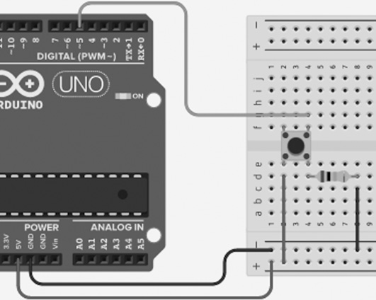
1.Add a push-button switch between f2 (top left) and e4 (bottom right) [f2–e4].
2.Add a 10kΩ resistor between pins [d4–d8].
3.Add a connector to the negative (ground) rail [c8–GND].
4.Add a connector to the positive (+5V) rail [d2–V+].
5.Add a connector between the bottom ground rail (near column 1) and the Arduino bottom left GND pin.
6.Add a connector between Arduino digital pin 5 and breadboard pin g4 [AD5–g4].
7.Add a connector between the bottom positive rail (also column 1) and the Arduino bottom left +5V pin.
The previous code listing can be extended to output the value of buttonInput to the Serial Monitor:
If this code executes correctly, when the push button is pressed you should see a change from 0 to 1 in the Serial Monitor output trace in Tinkercad (Figure 5.25).

If the code has compiled correctly and the circuit is configured properly, the previous listing can be extended to include a selection statement that tests the value of the digital input pin to execute different instructions in each case:
If the code compiles and executes correctly, you should now see the output trace shown in Figure 5.26 in the Tinkercad Serial Monitor window.

At this point, digital input can be read from a switch as the basis of a selection statement that executes different processes as a result. In the next example. this workflow will be used to control MIDI Note messages for output. Before doing so, there is one final aspect of selection instructions that can be included to further extend the flexibility of the system code – the else if statement (Figure 5.27).

In the diagram, the 1st condition (Condition A) is evaluated in the if statement. If the 1st condition is true then the selection executes Process A and the statement ends. If the 1st condition is false then the selection evaluates a 2nd condition (Condition B). Again, if the 2nd condition is true then the selection executes Process B and the statement ends. However, if the 2nd condition is also false then the selection executes the code inside the else statement (Process C):
In the listing, the additional else if statement allows multiple conditions to be tested at once. This means the number of inputs that can be processed can be increased, allowing the Arduino to respond to multiple sensors at the same time. There is one limitation of this statement, however: if condition A is true, then condition B is never evaluated. This is a crucial point in terms of the logic of the statement, as a priority has been created between the switches where switch A will always override switch B. This is not an issue for this example, but if this code were to be extended to select between more switches (i.e. a rudimentary MIDI keyboard) then a more flexible selection statement would be needed where all conditions are mutually exclusive of each other.
An else if statement is used in the next example, where two push-button switches are used to generate different MIDI Note messages for output through the Arduino MIDI interface. It is worth noticing that there are now six braces and four brackets (for the two conditions) in the code – it is becoming more difficult to keep track of the structure and processes involved. These issues will be discussed in the following short tutorial on how to code, to allow the more effective implementation of the subsequent MIDI switch example.
5.7 Tutorial – how to write code part II
The previous chapter introduced the concept of coding structure as a means of highlighting how code is not linear text. This chapter has covered a lot of conceptual ground, and it is important to take stock and revisit the structural and procedural elements of the code involved. The structural elements of both iteration and selection instructions are significant, and the use of brackets and braces (as with functions) requires a dedicated approach to writing them. The structures for iteration and selection are the best place to begin:
Before thinking about how often the loop has to iterate, or how best to define the condition, it is crucial to set up the structure of the statement. As the previous if/else if/else statement shows, six braces and four brackets leaves a lot of room for error. Comments have been provided on structures throughout the examples, and whilst this is not a method seen in most coding tutorials it is nevertheless a useful way of keeping track of iteration, selection and function stubs before they manifest an error due to a missing brace – often with a compiler error that points somewhere else.
The Tinkercad and Arduino IDE debuggers have not been discussed in any detail, as their proper integration into a coding workflow is outwith the scope of this book. Having said this, debuggers can often flag problems and errors with meaningful explanations if the coding structure is sound (particularly in shorter code examples), so it is recommended to do the following when code does not compile:
1.Count the brackets and braces – they should both be (separate) even numbers.
2.Check the semicolons – every sequence instruction must have one.
3.Check for missing loop elements – e.g. declaring the count variable type and that the end condition is correct.
4.Check for badly formed conditions – can the condition evaluate to true/false or LOW/HIGH?
5.Arrays and loops count from 0 – also, array elements must be initialized before use.
This chapter has covered most of the basic elements of computer programming that relate to the Arduino, but is not a substitute for coding experience – this will take time. Reading code written by others is a great way to learn, and unlike written work a lot of code is freely accessible for use by
others. This can often be a little surprising if you have never encountered computer programming before now:
Whenever possible, applying and amending code from other sources is arguably the best way to become proficient at programming. It is very rare, even after many years of coding development experience, that you will start writing any computer program from scratch. It is much more common to take code from other sources and adapt it to solve a problem. Whilst on some occasions this can cause problems (e.g. trying to understand third-party code that works, but doesn’t explain how!), in most instances the computer programming community are very helpful and supportive of those trying to learn new skills.
5.8 Example 3 – MIDI switch controller output
In this example, the previous MIDI output circuit is adapted to include two push-button switches. The code will also be reduced in some areas, by removing the array iteration previously used to generate a sequence of MIDI notes for output. In this example, a selection instruction responds to switch inputs by sending different MIDI Note data as serial output based on the condition of each switch (Figure 5.28).

This example contains the first full system that processes sensor inputs to create actuator outputs. A function called midiNoteOutput() has been added to handle the serialization of the note and velocity data for each message, partly to keep loop() from becoming too cluttered as it will now have an if/else if/else selection statement (with lots of brackets and braces to lose track of!). In addition, sending the three MIDI Note On bytes is a good example of when a function is needed – to reduce and reuse the code involved. The MIDI Note velocity byte can be used to effectively create a Note Off message by writing velocity 0 for the note – the code listing will show that this logic is deliberately simplified but not without some drawbacks as a result. An updated schematic can now be derived for the example, which combines switch inputs with serial output (Figure 5.29).
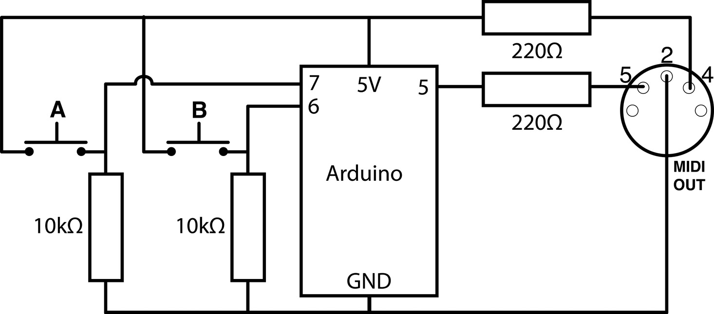
In the schematic, digital input and output are combined to produce a full MIDI OUT controller circuit. The switches provide +5V signal inputs to pins 6 and 7 when they are connected, with pull-down resistors being added to ensure no short circuits occur. The Arduino then processes these signals using a selection statement with two conditions (if/else if/else) to generate serial output to the standard MIDI OUT interface on the right of the schematic. This schematic can now be translated to a breadboard layout that can be prototyped (though not implemented) in Tinkercad (Figure 5.30).

The breadboard layout shown in the figure combines two digital switch inputs on pins 6 and 7 with a MIDI OUT interface (bottom right of the board). A similar circuit was used in the previous example, and this circuit extends it by bridging the power rails to provide access to both the top and bottom of the breadboard. The switches have 10kΩ pull-down resistors connected to GND, but the layout omits the LED serial tester circuit used in the previous example to keep things simple (these components can be added very quickly when needed for testing). As with the previous example, this circuit will be adapted again to build the MIDI drum trigger project, so a full build process is not provided at this point. For Tinkercad simulation and testing, the connection instructions for this circuit are as follows:
Switch inputs:
1.Add a push-button switch between f12 (top left) and e14 (bottom right) [f12–e14].
2.Add a 10kΩ resistor between pins [d14–d18].
3.Add a connector to the negative (ground) rail [c18–GND].
4.Add a connector to the positive (+5V) rail [d12–V+].
5.Add a connector between Arduino digital pin 6 and breadboard pin g14 [AD6–g14].
6.Add a push-button switch between f20 (top left) and e22 (bottom right) [f20–e22].
7.Add a 10kΩ resistor between pins [d22–d26].
8.Add a connector to the negative (ground) rail [c26–GND].
9.Add a connector to the positive (+5V) rail [d20–V+].
10.Add a connector between Arduino digital pin 7 and breadboard pin g22 [AD7–g22].
MIDI OUT interface:
1.Add a 220Ω resistor between pins [i1–i15].
2.Add a connecting wire from breadboard pin j5 to MIDI DIN pin 5 [j5–DIN5].
3.Add a 220Ω resistor between pins [i7–i11].
4.Add a connecting wire from breadboard pin j11 to MIDI DIN pin 4 [j11–DIN4].
5.Add a connector from the negative (ground) rail to MIDI DIN pin 2 [DIN2–GND].
6.Add a connector from Arduino digital pin 4 to breadboard pin j1 [AD4–j1].
Power connections:
1.Add a connector between the bottom ground rail and the Arduino bottom left GND pin [ADGND–GND].
2.Add a connector between the bottom positive rail and the Arduino bottom left +5V pin [AD5V–V+].
3.Add bridging wires on the right-hand side of the breadboard to link both sets of power rails (V+/V+, GND/GND).
LED test circuit:
1.Add an LED – anode pin (h5) to cathode (h6).
2.Add a connector to the negative (ground) rail [j6–GND].
3.Disconnect MIDI DIN pin 5 connecting wire at j5.
With the breadboard setup in Tinkercad, the code can be compiled to process digital switch inputs to generate MIDI serial data outputs. As the code for a complete digital system combines more complex processes, the listing will be covered in three sections to discuss each one individually:
The initial setup in this example involves both switch input and serial output. An input switch component has been added that requires additional code elements to use it. First, two byte variables (buttonOne, buttonTwo) are defined for the buttons that can either be digital 0 (LOW) or 1 (HIGH) depending on whether the switch has been pressed. Byte constants are then defined for the digital input pins involved (pins 6 and 7) – these pins must not change during the operation of our circuit, so it makes sense to declare them as constants. In the setup() function, the Serial and SoftwareSerial (SerialMIDI) objects are started so serial MIDI data can be output to the MIDI OUT interface circuit connected to digital pin 5. The pinMode() function is also used to configure pins 6 and 7 for digital input, so the switch voltage levels can be read from these pins. With the setup completed, the midiNoteOutput() function can be declared to output MIDI data bytes:
The function takes two input parameters – the MIDI note number and the note velocity. The status byte of a MIDI Note On message is hexadecimal 0x90, so with this information all three bytes of the message can be written to the SoftwareSerial output object that will output to the MIDI OUT interface on pin 5. Calls to the serial object are also included that write data to the Serial Monitor in Tinkercad, though these are commented in the listing as they are not needed when running the actual circuit. Recall that in example 2 three testing steps were defined, which this section of the midiNoteOutput() function focusses on:
1.Test the code – ensure that the function structure is correct before testing that the call to midiNoteOutput()from loop() is working (listing below).
2.Test the board – before connecting the LED serial test circuit, use the Serial Monitor calls to check data is being built and transmitted by the ATMega328P.
3.Test the system – the full MIDI controller system cannot be tested until the code and board are running correctly.
With the midiNoteOutput function declared, it can now be called from the selection statement in loop():
In loop(), the selection statement if/else if/else structure must be coded before adding the instructions that will be executed in each case of the condition. This is important to avoid introducing simple errors into the code due to a missed bracket or brace, alongside checking that the logical if/else if/else structure is built correctly. Each stage of the selection statement is commented to avoid this problem – there are now eight braces in loop(), and they can easily get confusing! The digital state of the buttons can then be obtained by calling the core Arduino function digitalRead(), which will return either a LOW (0V) or HIGH (+5V) based on the voltage level measured on pins 6 and 7. The result of these calls is then stored in the buttonOne and buttonTwo variables, so they can be evaluated in the selection statement.
The logic of the selection statement aligns with the code process diagram shown in Figure 5.28, where each condition relates to one of the input push-button states. The end of section 5.6 noted the important of else: else means everything else. This point is demonstrated here, where all MIDI notes must be off to prevent a switch triggering a note of indefinite length (anyone who has worked with MIDI for a long time will have experienced occasions when the system must be disconnected to turn off rogue note messages!). This is handled in the code by setting the default else condition to all notes off, but this has a limitation – what happens if switch A is held down and switch B is pressed at the same time?
The selection structure will prioritize switch A over switch B, so in practice switch A will always trigger in this case. Thus the system will not respond adequately to this condition, creating a monophonic (single signal) MIDI controller as a result. This is not a significant issue for this example as the focus is on building a first complete system from input to output. Having said this, in a practical MIDI controller the limitation of monophonic operation can have significant practical implications for chords and other concurrent note patterns (such as faster note sequences).
The Tinkercad simulation should run this code correctly and trace out MIDI Note On messages to the Serial Monitor (Figure 5.31 overleaf).

At this point in the example, the Tinkercad simulation will not be able to work with MIDI data and connectivity (other than running the LED serial test circuit). The code and (to some extent) the board have been tested, but not the overall MIDI system that will be controlled by the MIDI data. Whilst the aim of this book is to provide full step by step examples throughout this book to avoid any ambiguity or confusion, the focus in this section is to introduce the processing of digital input within the system – not build a full circuit. This is the first full Arduino system in this book, and although this circuit will not be built step by step it still represents a significant advance in your learning. Sensor inputs can be evaluated using selection statements, and the outcome of a condition can execute different processes contained within a dedicated function. In the next section, this will be extended by learning how to measure analogue input signals with the Arduino. This will lead onto the final project of a MIDI drum trigger system that will output through a standard MIDI OUT hardware interface – a fully functional MIDI control system.
5.9 Analogue input – percussion sampling
In the previous section, switch input worked on the premise of a discrete digital signal being present – the switch output would either be LOW (OV) or HIGH (+5V). Chapter 2 (section 2.2) discussed continuous signals, where the voltage level of the signal continuously varies over time (Figure 5.32).

In the diagram, a continuous signal constantly varies in level over time – this distinguishes it from the digital signals in the previous section, which were always at one of two specific voltage levels. The diagram also shows where the signal exceeds the measurement range for illustrative purposes, as in reality the problem of measurement is compounded by the sample rate and bit depth available (as briefly discussed in chapter 2). Thus, when sampling a continuous signal accuracy is lost due to lack of sampling resolution (Figure 5.33).

In the diagram, the effects of sampling a continuous waveform are shown in the right-hand signal, where simple nearest-neighbour interpolation has been used to highlight the gaps between the data points. Although in practice more advanced interpolation methods would be used for audio signals, they require more processing power than that available on the ATMega328P. On the Arduino, analogue signals can be measured as inputs on pins A0–A5, where they are converted to data values by analogue to digital conversion (ADC), using the Arduino power supply (5V) as a reference for measurement. The maximum input value is 5V because the Arduino cannot operate above 5V, so it cannot measure any voltage higher than this (it would not have a voltage to compare the input signal with).
The Uno can sample an input signal at 10-bit/10kHz resolution, and chapter 2 (section 2.3) showed that the bit depth is the number of values (the range) that can be used to represent the input signal. Section 2.2 also (briefly) covered binary, where the small number of values in binary (either 0 or 1) means that a large number of digits (known as binary bits) are needed to represent a quantity. The range of values for a given bit depth can be calculated by taking the number of binary values (2) and squaring it by the number of bits:
 (5.1)
(5.1)Note: 2 is a scalar representing the number of binary values (either 0 or 1).
Thus, a 10-bit binary number provides a range of 1024 values, which will equate to an integer type in the code. This means that the Arduino can represent an input voltage between 0V and 5V (Arduino supply) using a range of 1024 values, giving an input resolution of:
Note: this assumes a supply of 5V (the Arduino can also run on 3.3V).
Whilst a 10-bit depth is more than adequate for many types of input sensors (e.g. switches, potentiometers) you will be familiar with 16-bit (e.g. compact disc) and even 24-bit audio formats that provide a much greater range of input signal measurement (24-bit gives a range of 16,777,216 values). With a resolution of 4.9mV, the Arduino should be able to read our sensor input with a sufficient level of accuracy. Although in audio-processing terms this would not be acceptable, for this use of sampling to detect input sensor changes the definition of a threshold (see below) based on a much lower resolution allows a simpler approach to be taken when processing the data obtained.
Chapter 2 (section 2.3) discussed the effect of reducing/increasing the sample rate, where just as with bit depth a lower sample rate also reduces the resolution of the digital representation of the signal. The Arduino also does not have enough memory or a high enough clock speed for audio sampling, and whilst this book will not provide an extended discussion on Nyquist’s theorem, it is sufficient to remember that the minimum frequency being sampled must be at least half of the sampling rate. For sensor input however, with a sampling rate of 10kHz the Arduino is again more than adequate for the input sensors used in this book:
 (5.3)
(5.3)Note: in practice, processing each sample will take much longer.
To provide some perspective, a sample resolution of 1 millisecond means it can theoretically detect all musical note durations within a wide range of tempos (Figure 5.34).
|
Beats per minute (BPM) |
Note duration (milliseconds) |
|||||
Whole |
1/2 |
1/4 |
1/8 |
1/16 |
1/32 |
|
60 |
4000 |
2000 |
1000 |
500 |
250 |
125 |
80 |
3000 |
1500 |
750 |
375 |
188 |
94 |
100 |
2400 |
1200 |
600 |
300 |
150 |
75 |
120 |
2000 |
1000 |
500 |
250 |
125 |
62.5 |
140 |
1716 |
858 |
429 |
215 |
107 |
53.5 |
160 |
1500 |
750 |
375 |
188 |
94 |
47 |
180 |
1332 |
666 |
333 |
167 |
83 |
41.5 |
200 |
1200 |
600 |
300 |
150 |
75 |
37.5 |
The figure shows common note durations for a range of tempos, to illustrate the difference in time resolution between a 37.5 millisecond demisemiquaver note at 200 bpm and the much higher sampling resolution of the Arduino at 1 millisecond. This table aims to clarify both the detectable time resolution of a sensor input (which is much smaller than most musical notes!) and also the response time of a processor like the ATMega328P (which runs at 16MHz cycles per second). With such high resolution in both sampling and clock speed, it would seem feasible that timing will never be an issue – the ATMega328P can easily generate serial MIDI Note On messages at the output rate required. This is noted in advance of building the MIDI drum trigger project, where the effective responsiveness of the trigger is not based solely on the resolution and execution speed of the Arduino. In practice, the input signal must also be measured relative to a threshold to define when the input sensor data is either digital HIGH or LOW (Figure 5.35).

In the diagram, the fast onset time of the signal (known as the attack) is typical of the striking collision that generates a percussive sound (often called a drum stroke). The decay of the sound (known as the release) is also quite rapid, and the critically damped sine wave shown is close to that of a bass drum sound (particularly for electronic drums). The next chapter will discuss analogue audio signals (and the crucial role of sine waves) in more detail in relation to AC circuit theory. For now, the detection of the first onset threshold of a piezo input sensor can be used as a MIDI drum trigger. To do this, the Arduino must sample the continuous analogue input signal from the piezo and then use a condition to determine when this sampled value goes above the defined threshold. The threshold must be greater than 0, but the circuit must be tested to determine where the best value will be to help avoid multiple onset detections from the same sound (as shown in the right-hand diagram in Figure 5.35). The threshold must also be used to avoid detecting other vibrations that are not related to the actual drum stroke that produces the percussive sound (see Figure 5.36 overleaf).

The diagram gives some basic examples of the multiple sources that can occur within a percussion signal – the sensor does not discriminate on their source, it simply detects all vibrations. These additional vibrations manifest as noise in the input signal, and thus the threshold is used to avoid detecting them. This creates another problem if the threshold is set too high to avoid false triggering due to noise – the potential range of input signals is now reduced to detect only the very loudest sounds (Figure 5.37).

Too low a threshold can lead to the detection of multiple onsets, but the threshold level must also not be set too high – thus reducing the sensitivity of the trigger. These issues are discussed to highlight the complexity involved in building a fully functional MIDI drum trigger interface – the difference between this simple Arduino example and a commercial interface is a significant amount of design, modelling and testing to develop accurate onset detection across a wide range of drums and percussion. For this project, an initial threshold value can be set in the code to get things working – a selection statement can then be used to evaluate whether the input signal has reached (or exceeded) this value:
In the loop() function, the value of the analogue input pin is obtained using analogueRead() and then stored in the variable inputSignalLevel. This variable is then used to evaluate the result of the expression inputSignalLevel > inputTriggerThreshold in the selection statement. The mathematical symbols for greater than (>), less than (<) and equivalent to (==) are widely used in selection statements to evaluate a quantity, where the result of the expression is either a Boolean true or false. This means the condition is only responding to samples obtained from the piezo sensor that are above the defined threshold.
To obtain this sample data, we declare an integer to hold the input from our piezo sensor. We use an integer type as the Arduino has 10-bit input resolution, which we know gives a range of 1024 possible input values. Next, we declare a constant integer for the analogue input pin we will connect the piezo sensor to. This can seem a little confusing as we seem to be assigning the value ‘A0’ to an integer, but actually in the Arduino pin assignment header code (which you do not need to learn!) all analogue pins are defined as A0/A1/A2/etc. and then mapped to specific pin numbers that begin after the digital pins (A0 is actually pin 14, A1 is 15 and so on).
An initial threshold value of 200 is declared, which is in the bottom 20% of the overall range of 0–1023. This value can be tested in the final project to find the best balance between input sensitivity and signal-to-noise ratio, knowing that any vibration near the piezo sensor will register at some level. If testing produces false triggering because the value is too low it can be amended upwards, or conversely reduced if there is a lack of sensitivity to input. The condition evaluates true if inputSignalLevel > inputTriggerThreshold and if this is the case a MIDI Note On message can be sent using a function call (as in the previous example). This may seem reasonably straightforward, but there is also a second condition that must be taken into account – what happens after the first onset value, when the sampled values that follow it are also still above the threshold (Figure 5.38).

In the diagram, there are two specific samples of interest – the first sample above threshold (onset), and the first sample after the signal crosses back down below threshold again (offset). These events equate to MIDI Note On (onset) and MIDI Note Off (offset) messages that will define a drum stroke, but they must be separated out from all the other samples that are higher than the defined threshold. The MIDI Note On message must only be sent once when the input signal reaches threshold – no other onset should be registered until the signal goes below the threshold again. This requires a second condition for the input signal that checks to see if a previous MIDI Note On has occurred, which can be implemented in the selection statement using Boolean algebra:
The concepts of conjunction and negation will be introduced using code examples, as a full discussion of this topic is beyond the introductory programming concepts discussed in this book. Having said this, if you wish to progress into digital electronics then you will inevitably encounter truth tables as a useful way of defining all the logical outcomes for a specific set of conditions (Figure 5.39).

This second condition is defined by a Boolean variable named noteTriggered, which is set to true when a MIDI Note On is sent. Thus, noteTriggered is only true when a MIDI Note On has happened and so other samples over threshold can be ignored. This means the conditions can be combined to only respond to the first sample over threshold by testing for !noteTriggered – which equates to NOT noteTriggered (false). Once a MIDI Note On message is sent, this can be set to noteTriggered = true to ensure that any following sample over threshold does not meet the combined criteria of >inputTriggerThreshold &&!noteTriggered. To do this, extra brackets must be added to each part of the selection statement to make sure each condition is evaluated separately:
In the listing above, the threshold (inputSignalLevel > inputTriggerThreshold) is evaluated as the first condition (hence the brackets). Then both conditions are evaluated together in the full conjunction statement ((inputSignalLevel > inputTriggerThreshold) && !noteTriggered). A conjunction statement means A AND B – as denoted by the && symbols. This means that when the sample is greater than threshold AND noteTriggered is false (!noteTriggered) a MIDI Note On message is sent.
In the second else if statement, (inputSignalLevel < inputTriggerThreshold) is now evaluated and it is crucial to note the change to less than (<). This condition will only be true when a sample is less than threshold, which is the same as saying >inputTriggerThreshold = false. Now this result can be evaluated within a second conjunction statement ((inputSignalLevel < inputTriggerThreshold) && noteTriggered) to find the first sample after a MIDI Note On that has crossed below the defined threshold. When this condition is true, a MIDI Note Off message can be sent to terminate the previous MIDI Note On – thus avoiding sending a note that does not switch off.
As previously noted, an in-depth discussion of conjunction and negation to evaluate combined logic conditions is beyond the scope of this book, but examples are provided to allow a full MIDI drum trigger project to be built in the following section. It is recommended to consult more comprehensive programming tutorials and texts on this topic to help disambiguate both these concepts and their application. Combinatorial logic takes a significant amount of time to understand and can prove to be a major source of programming problems. For now, the final project will build the first full practical system in this book, in part to define a milestone in your learning and also to provide you with the building blocks needed to extend this project in the future if you so wish.
5.10 Final project: MIDI drum trigger
The MIDI drum trigger project combines both the electronics and programming topics covered in the book so far, where Arduino code is used to read an input sensor (piezo) value and select the specific circumstances for which this input will generate a MIDI Note On (or Off) message as output to a serial MIDI OUT interface. Before beginning, take a moment to remind yourself how much you have learnt in a short space of time – this project combines DC circuit theory with Arduino C programming to build a full MIDI control system that is compatible with any standard MIDI interface, and represents a significant learning milestone in this book. As stated, the MIDI Drum trigger system uses the Arduino to sample and analyse piezo sensor input to create serial data output in the form of MIDI messages (Figure 5.40).

The main element of the Arduino code process is the if/else if/ else statement that evaluates the combined threshold and noteTriggered conditions to determine the first onset and offset of the input drum stroke. Notice that both conditions in the selection are reversed in each case relative to the MIDI Note message they relate to, while the else condition has no output:
1.Note On Condition: >threshold && !noteTriggered
2.Note Off Condition: <threshold && noteTriggered
The schematic for this system is fairly similar to the previous example systems in this chapter, where a sensor input is connected to the Arduino, which then sends serial data as MIDI Note messages to the 5-pin DIN MIDI interface as output (Figure 5.41).

A piezo sensor is polarized, so like an LED it must be connected in the correct direction to avoid damaging the sensor. In addition, a piezo sensor can generate a large output voltage (some piezos can produce between 50 and 90V) that is well outwith the Arduino input range of +5V. Chapter 3 (section 3.4) showed how the voltage in each parallel branch of a circuit is constant because electrons have the same potential to move down any available branch. In this circuit, a large resistor is connected in parallel to the piezo to prevent the piezo from creating a larger input voltage than the Arduino can handle – recall that larger resistances make no real difference in a parallel circuit (see chapter 3 section 3.1.5 Q9). From the schematic, a breadboard layout can be created for the entire MIDI drum trigger circuit (Figure 5.42).

A PCB mount screw terminal block is used to connect the piezo sensor to the breadboard (Figure 5.43).

Screw terminal blocks help to prevent the audio wires from moving and becoming detached from the breadboard (which can easily happen with a direct wire inserted into the breadboard). When connecting a wire to the block, it can help to pre-mount the terminal block to the breadboard to provide a solid surface to work with. To insert the wires, it can be easier to unscrew one terminal on the block, and with a wire in position (inside the terminal clamp) screw the terminal to clamp down on this wire while holding it in position (the figure shows how tweezers can be used for this).
In the case of two wires (either for a piezo sensor or for an audio connector as used in chapters 7–9), one common issue can be too much exposed wire outside the terminal block. This can potentially short out the signal by allowing both wires to make contact with one another outside the terminals – so the terminal effectively becomes a short circuit. It is recommended to take a little time when stripping the wire for connection to ensure that a relatively short (<1cm) length of wire is exposed. With the breadboard layout completed, we can now enter the code needed to process piezo sensor switch input to generate MIDI serial data output.
Full code listing
In the listing above, you should already be familiar with much of the selection statement code used to capture the first sample above threshold (onset) and the first sample after this that crosses below threshold (offset). The same midiNoteOutput()function from the previous example is used to send MIDI Note messages to the SoftwareSerial object for output to a MIDI OUT interface. If you copy/paste this code directly into the Arduino IDE, it should compile and upload onto your Arduino board. From here, the first full system prototype can be built.
Project steps
For this project, you will need: 1. Completed circuit from previous build (sequence player) 2. 1 × 2 pin screw terminal block connector 3. 1 × piezo sensor 4. 1 × 1MΩ resistor 5. 1 × connector cable and 3 × connector wires |
|
Piezo Sensor Input: 1. Add a 1MΩ resistor between pins [g18–g22]. 2. Add a connector wire before the resistor to breadboard pin e18 [f18–e18] – this is the parallel path for the piezo sensor. 3. Add a connector wire after the resistor to breadboard pin e20 [f22–e20] – this completes the parallel path for the piezo sensor. 4. Add a connector wire after the resistor to the negative (ground) rail [j22–GND]. |
|
1. Connect the Arduino analogue input pin A0 to pin h18 (Arduino connection not shown) [ADA0–h18]. |
|
1. Connect the piezo sensor wire to a screw terminal block – if the wires are too long, they can be looped and twisted until they are shorter (only looping will allow them to move around inside the screw terminal block). |
|
1. Connect the screw terminal block between pins c18 (positive) and c20 (negative) to leave space for the connector wires. |
|
To add the LED test circuit: 1. Add a 220Ω resistor between pins [g11–g15]. 2. Add an LED – anode pin (f15) to cathode (f16). 3. Add a connector to the negative (ground) rail (j16-GND]. 4. To test serial output, connect the Arduino digital pin 5 connector to pin f11 (not shown). |
|
|
|
Connect the piezo sensor to the underside of a drum practice pad. Any surface that is robust enough to withstand drum strokes can be used, but sensor performance will vary. |
|
Using whatever MIDI equipment you have available (either synthesizer or computer MIDI interface) connect a MIDI cable between your Arduino breadboard DIN socket and this system. Configure your system to receive MIDI data on channel 1. If the system functions correctly, every time you strike the drum pad a MIDI Note On message should be sent on channel 1 to your MIDI system. With some tweaking of the input threshold, a usable drum trigger can be obtained.
|
|


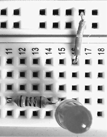


If you are not getting a usable output from your system:
1.Test the code – the inputTriggerThreshold value may be too high (or low).
2.Test the board – recheck pin connections – are the piezo wires properly connected to the screw terminal block.
3.Test the system – connect another MIDI interface to ensure it is responding to messages on channel 1.
5.11 Conclusions
As with the previous chapter, this chapter has provided an introductory overview to C programming for the Arduino and so has covered a lot of ground in a short space of time. The chapter began by discussing arrays as logical structures for grouping variables and showed how a for loop can be used as an iteration instruction to process each element of an array in sequence. An array was used to hold a sequence of note frequencies for output to a piezo loudspeaker using pulse wave modulation (PWM) on an Arduino digital pin, where PWM can also be used to output a voltage range between +5V (HIGH) and 0V (LOW). The chapter then covered serial output on the Arduino, and how the SoftwareSerial object allows other digital pins to be used to send digital data (as pins 0/1 are also used by the USB interface that connects the Arduino IDE to our board). The SoftwareSerial object was then used as part of a standard MIDI OUT interface that sent a sequence of MIDI Note On messages (in running status) using note numbers held in an array. This MIDI OUT interface is built to the standard MMA 1.0 specification, and thus should be interoperable with all other MIDI interfaces that use a 5-pin DIN connector.
The chapter looked at how the Arduino can receive and analyse input using selection instructions – the last of the three core programming instruction types. Selection instructions can become complex (and take time to learn), so were introduced by example only. An if/else if/else selection was used to process two push-button switches for MIDI output, to show how digital input can be analysed by the Arduino to create a full electronics system that combines input/process/output. In so doing, the three stages of testing needed when working with a full Arduino system were introduced:
1.Test the code – check the code compiles, run software tests in Tinkercad (also with the LED serial test circuit).
2.Test the board – component layout must align with the schematic, and all circuit paths must be checked.
3.Test the system – once software output is confirmed (Serial Monitor) we must test with a full system.
Selection statements were then extended to work with analogue input from a piezo sensor, which required two conditions – one for threshold to indicate onset/offset and a second condition to prevent multiple MIDI Note messages being sent. This logic structure was used to build a full electronics system that takes input from a piezo sensor, processes this input using the Arduino and then outputs MIDI Note messages as a result. This system represents a learning milestone in this book, combining audio systems design, DC circuit analysis and Arduino C programming to produce a fully functional MIDI drum trigger system.
The next chapter will move on to a completely new topic – alternating current (AC) circuits. Audio signals are continuous, they change over time. Working with continuous signals requires an understanding of the relationship between sine waves and audio signals in terms of both their magnitude and phase. This leads to the definition of impedance as the AC form of resistance, where the varying nature of the signal means a magnitude value cannot be calculated in the same way as DC circuits in chapter 3. This leads on to time-varying components like the capacitor, which are a core building block of all electronic circuits. Capacitors will be used in various parts of the amplifier and filter circuits later in the book, where the frequency-dependent nature of the component provides control over input and output audio signals. The mathematics involved in AC circuits are more complex than in DC circuit analysis, but ultimately the same basic principles apply.
5.12 Self-study questions
As this chapter represents a learning milestone in the book, no self-study questions are provided at this point. Instead, consider the following:
1.Reflect on how much you have learned about audio systems, DC circuits and Arduino programming in a short space of time – we often focus on what we don’t know and forget what we have learned! Also spend some time re-reading the chapter summary sheets – do you know how the concepts involved relate to the final project in this chapter?
2.Think of how the current project could be improved or extended to make it a more practically useful system. For example, you could add multiple drum triggers to output on different MIDI Note numbers. You could also perform input velocity triggering where you map the sample value range (0–1023) to the MIDI velocity range (0–127). You could even add MIDI channel assignment where you increment a channel number variable using a push-button switch
3.Take a short break from this book to let what you have learned fully sink in – the desire to progress can often slow your learning down if you do not take a break in your studies. The next chapter will focus on AC circuit theory and thus does not provide many practical examples, so you will need a break to help refocus your thinking from the very practical coding work covered in both chapters 4 and 5.