Search in book...
Toggle Font Controls
Create new playlist

Name your new playlist

Playlist description (optional)
Sign In

Email address

Password

Forgot Password?

or

Continue with Facebook

Continue with Google
Sign Up

Full Name

Email address

Confirm Email Address

Password

or

Continue with Facebook

Continue with Google

In this chapter, we will learn how to analyse direct current (DC) circuits. The basic principle behind DC circuits is that they are time-invariant – they do not change. This means we can specify voltage and current values and assume that these will remain the same as long as the power supply to the circuit is connected, which differs from the alternating current (AC) circuits we will encounter later in the book. This chapter represents our first real introduction to electronic circuit analysis, where we will learn the basic equations and rules of series and parallel circuits. You may find the maths in the chapter examples takes a little time to work through (particularly for parallel circuits) but remember that the equations themselves are quite straightforward – it’s the scales and symbols that take some time to get used to. We will begin by learning about Ohm’s Law, a fundamental equation that defines the relationship between voltage, current and resistance in a circuit. Ohm’s Law was briefly introduced in chapter 1 as an example of a relatively straightforward equation used in electronics, and now we will learn how to work with it in practical terms. We will also encounter two other fundamental aspects of DC circuit analysis – Kirchoff’s Voltage Law (KVL) and Kirchoff’s Current Law (KCL). These two laws are used in all electronic circuits, so this chapter will spend a little time deriving them and explaining their use. We will use KVL to analyse series circuits (where all components are connected in a single loop) and KCL to analyse parallel circuits (where current can travel down multiple branches within the circuit) demonstrating the following rules:

series circuits – voltage varies and current is constant

parallel circuits – current varies and voltage is constant

A short tutorial is provided showing how Ohm’s Law and KVL were used to derive the resistor value for our LED circuit in chapter 1 – explaining why the value of 150Ω was used in that circuit. The final projects compare series and parallel LED circuits to show the practical differences between them. Unfortunately they are not particularly exciting (nor audio-related) projects, but they will give you more practice with Tinkercad, circuit design and breadboard layout to get familiar with the practicalities of building real circuits.

3.1 Ohm’s Law and direct current

Chapter 1 introduced the three fundamental elements needed to begin learning about electronic circuits:

We also used the Arduino in our first project to power a simple circuit with a resistor and an LED as output, intending to look at this circuit in more detail in this chapter. As a first step, we can reduce this circuit to its minimum functional level by removing the LED output, so we can learn how to use circuit analysis techniques to determine the value of the resistor in the circuit (Figure 3.1).

Figure 3.1A simple Arduino circuit. The left-hand diagram shows an Arduino providing 5V to power to a single resistor. The right-hand diagram shows the schematic representation of the Arduino as a standard 5V DC voltage source. This is the simplest circuit we can design, though in practice it does not provide any inputs or outputs and so is not a practical system.

In the example circuit in Figure 3.1, a single resistor is connected to the Arduino 5V output to create a circuit path to ground (GND). The right-hand schematic shows the same circuit with the standard symbol for a DC voltage source, which includes the polarity (+/−) of the circuit for conventional current flow (see next section). The following examples will use a DC voltage source unless we are building a project circuit, in which case the left-hand representation will show the Arduino as a power supply. Although this circuit does not do anything useful, it allows us to consider a practical constraint of Arduino output when connected over USB. As we saw in chapter 1 (Table 1.2), the USB protocol defines a maximum current of 500mA for connected devices so our Arduino (which will draw power from the computer that programs it) will only be able to supply a current up to this value. If the Arduino can output a maximum current of 500mA through its 5V pin, the resistor in our circuit should limit the current to this value (though in practice the computer will limit the supply regardless). To determine a suitable value for this resistor, we use an equation introduced in chapter 1 – Ohm’s Law:

Voltage, V=IR $V o l t a g e, V = I R$

(3.1)

	$V$ $V$ is the potential difference in volts (V)
	I $I$ is the current in amperes (A)
	R $R$ is the resistance in ohms (Ω)

George Ohm developed the equation above in 1827 to show that the potential difference (V) between two points on a wire is equal to the magnitude of the current (I) flowing through it multiplied by the resistance (R) of the wire itself (Figure 3.2).

Figure 3.2Resistance and Ohm’s Law (taken from chapter 1, Figure 1.11). In the left-hand example, the lower resistance will not significantly impede current flow, so the difference in charge (potential difference) between the ends of the wire will be lower. In the right-hand example, the higher resistance prevents charge from flowing easily, creating a greater difference between the number of free electrons at each end of the wire.

In Figure 3.2, because the wire resists the flow of current, more charge builds up at one end of the wire than the other. As a result, the imbalance in electrical charge between the two ends of the wire creates a potential difference. For a lower resistance value, the imbalance is not as significant. as more current can flow through the resistor and so both points have similar levels of charge. For a higher resistance value, the reduction in current flow means more charge is now concentrated at one end of the resistor as it cannot flow easily to the other end. This increased resistance creates an increased imbalance in charge, which creates a higher potential difference between the two ends of the wire as a result. We know that the current does not change because the number of electrons stays the same, the only difference is where the electrons are located. Thus, we can see that increasing R increases V, so we can derive Voltage, V=IR $V o l t a g e, V = I R$ .

Scales, symbols and equations

In chapter 1, we learned that fundamental electronics equations are not mathematically complex, but the scales and quantities involved can take time to learn. Ohm’s Law defines the simple mathematical relationship between the three fundamental elements of voltage (V), current (I) and resistance (R), but the symbols involved can initially appear a little confusing. The letter (I) is used for current partly because it was originally discovered by André-Marie Ampére, who as a French speaker named the quantity Intensité du Courant (Current Intensity). In addition, electrical charge is measured in coulombs (C), which would also create a confounding between terms! As you progress through the book you will find that scales and symbols often take more time to learn than equations, so terms will be explained whenever they are first introduced.

Ohm’s Law is a simple equation to work with and forms the basis of all electrical circuit analysis. We can apply the equation in different ways, where we can use any two of the quantities involved to determine the third by simply rearranging the terms:

V o l t a g e, V = I R C u r r e n t, I = V R R e s i s t a n c e, R = V I

$V o l t a g e, V = I R C u r r e n t, I = \frac{V}{R} R e s i s t a n c e, R = \frac{V}{I}$

(3.2)

This rearrangement of quantities is a very important analysis tool, and we can use our circuit example from Figure 3.1 to show how Ohm’s Law can derive the correct size of resistor needed to limit the current in the circuit to 500mA.

3.1.1 Worked example – calculating a resistor value

This example uses the simple circuit from Figure 3.1, though it has no practical use other than to introduce Ohm’s Law for calculation.

Q1: A single resistor is connected in a circuit powered by a 5V voltage source (from an Arduino). As the Arduino has a maximum output current of 500mA, a resistance value is needed to limit the output current to this level – what would be a suitable value for this resistor?

Answer: A suitable resistor value for the circuit would be 10Ω.

The example above is simple enough, though of no actual practical use – the Arduino is limited by the USB protocol of the computer supplying it, so it cannot exceed 500mA even if the resistance in the circuit was lowered to 5Ω (giving a theoretical current of 1A). It is also important to note that all Arduino output pins are limited to 40mA and driving them beyond this current will damage the Arduino (the +5V power pin is not directly connected through the microcontroller so it is not limited in this way). The purpose of this circuit is to show how straightforward Ohm’s Law is to use, providing you know two of the three quantities and pay attention to any scaling factors involved. As you progress through the book, we will use Ohm’s Law extensively in our circuit analysis so it will help to spend some time looking at equation (3.2) to become more comfortable with rearranging the terms involved. Now we have learned how to apply Ohm’s Law, we can move on to another set of fundamental laws that define the behaviour of electronic circuits – Kirchoff’s Circuit Laws.

3.2 Kirchoff’s Voltage Law: series circuits

Chapter 1 discussed analysing circuits using conventional current flow, where it is (incorrectly) assumed that charge flows from the positive to negative terminal in the circuit. We learned that this is a result of historical precedent, where electrical charge was originally believed to be positive long before the negatively charged electron was discovered. Aside from the reason for the difference in current direction, note that in electronic circuit analysis the direction of the current does not actually make a difference – as long as we calculate in a single direction (Figure 3.3).

Conventional current flow

The idea of maintaining a single direction for analysis can seem either obvious or arbitrary (or both!), but in many ways it is not unlike adding (2+3) or (3+2) – regardless of the direction in which we add the quantities, the result is still 5. In practice, the flow of electrons may be in the opposite direction to our analysis but the answer to our equations will remain the same if we are consistent in the direction used.

This seems to be quite straightforward: as we have noted the reason for this historical precedent so we can then move on to its application. The problem occurs when trying to reinforce our conceptual understanding of voltage, current and resistance whilst also learning to use Ohm’s Law and Kirchoff’s Laws – it is then we may discover that thinking in reverse can be more difficult than it first appears! The solution is to proceed slowly to reiterate the concepts learned in chapter 1, while learning to use the new analysis methods introduced in this chapter. If you remember to do this, the conceptual gaps in your understanding will not become wider as we progress.

We measure current as the flow of charge over time in a single direction – this is known as direct current (DC). In a DC circuit, the current and potential difference at any place in the circuit are constant – they do not change over time. In chapter 2, we learned about continuous time (CT) signals (also known as analogue) that carry input from sensors like microphones and also drive output to loudspeakers – CT signals vary over time. In chapter 8, we will learn about alternating current (AC) as a means of building circuits for CT audio signals, but for now we will focus on DC circuits to help us understand and apply basic circuit analysis techniques.

In 1847, Gustav Kirchoff defined two fundamental laws that govern the behaviour of all electronic circuits. We will look at each of these in turn as they apply to series and then parallel circuits, beginning with Kirchoff’s Voltage Law (KVL):

This law is fundamental to all electronic circuits, and will be used extensively in this book. The key to understanding this law is to define the polarity of the voltage drops, to ensure we know the direction of each potential difference within a loop. This can be a little confusing at first, as the potential difference across a voltage source in a circuit is in the opposite direction to the potential difference of the resistance connected across it (Figure 3.4).

Figure 3.4Voltage polarity in a series circuit. The diagram on the left shows the direction of the potential difference (low to high) across a voltage source and the subsequent direction of the voltage drop through a series resistor connected in this circuit. The diagram on the right shows a rearranged version of the same circuit, to highlight the opposite direction of the potentials involved.

This diagram shows a series circuit: a single loop in which all components are connected together in series. We have already used Ohm’s Law in the previous section to determine the value of a resistor in a series circuit but as noted in the previous sidebar, at this point you are synthesizing several concepts at the same time: conventional current flow, voltage (potential difference) polarity and Kirchoff’s Voltage Law (KVL). For this reason, it is useful to step through each of these elements in turn to be clear about how they relate to one another – you may understand them all individually, but combining them can lead to comprehension problems when you are beginning circuit analysis:

1.Conventional current flow – we know the direction does not impact on circuit analysis but it does require us to reverse our thinking in terms of the flow of charge. Although we know electrons flow from negative to positive, we must now think of current as flowing from positive to negative.

2.Voltage polarity – We define the direction of potential difference as being from low to high, to show the difference in polarity between the voltage source and resistor (second image in Figure 3.4). Consider that the arrowhead indicates the direction of movement of charge, where a resistor opposes the flow of charge from the voltage source. This can be confusing when you try to combine your thinking with conventional current flow to imagine how electrons would move, so take some time to consider this point as being both conceptual (polarity) and practical (conventional current).

3.Kirchoff’s Voltage Law – as mentioned above, the key to understanding KVL is to see voltage polarity as being the direction of potential for charge to flow. If you are comfortable with step 2 then realize that the potential difference of the resistor is being subtracted from that of the voltage source – they will cancel each other out to give a total of zero volts.

From KVL, we can now see that because all the voltage drops in a loop must equal 0, the voltage source ( VS $V_{S}$ ) is effectively being opposed by the resistor voltage ( VR $V_{R}$ ). This means that VS−VR=0 $V_{S} - V_{R} = 0$ and by rearranging the equation VS=VR $V_{S} = V_{R}$ . To think of this another way, the voltage source provides the potential difference needed to move charge around a loop and other circuit components (i.e. the resistor) reduce it – they cancel each other out.

Current in a series circuit

We have learned that different voltage polarities determine how components resist the flow of charge from a source by cancelling each other out. In addition, if a voltage source is the only component in a loop providing free electrons then the current in that loop will not change – it will remain constant at all points. This can initially be a little confusing, as we have learned that current (amps) is the rate of electrical charge (coulombs) per second. If this is the case, then it can seem logical that the electrons ‘slow down’ after entering a resistor and so the current would thus vary on either side of the resistor.

In fact, electrons do not change speed – we are simply counting their number at a particular point in the loop for a specific length of time. If fewer electrons can flow out of a resistor, then fewer electrons will flow into a resistor – the resistor has reduced the number of electrons moving throughout the circuit. Thus, the current in any series loop is limited by the total resistance within it – all electrons will move the same overall distance, regardless of whether they are currently inside (or outside) any particular resistor:

The image above shows how combining a low and high resistance effectively reduces the overall current flowing in a circuit, where current is measured as the amount of charge (in coulombs) flowing past a given point in one second. As there is less area in the higher resistor for electrons to move, the number of electrons that can pass any given point will be reduced. Thus, in the second example the distance an electron can travel within the lower resistance is also now reduced – there is nowhere else for it to go. A simple analogy would be to think of electron flow through multiple resistors like a traffic jam, where cars on a multiple-lane road move less overall distance because the nearest exit ramp only allows single-lane traffic to leave.

As free electrons can only enter through the voltage source, in series circuits voltage varies and current is constant.

Now we know that all voltage drops in a loop will cancel each other out to zero, and also that the current in that loop will be constant. By combining these two elements with Ohm’s Law, we can develop a simple equation for determining the total resistance in a series circuit (Figure 3.5).

Figure 3.5Calculating total resistance in a series circuit. *In the diagrams, examples of series circuits combining two and three resistors are shown. We know that the supply voltage (V*_S) is equivalent to all component voltage drops, and that current in the loop is constant. By rearranging the terms, we can derive the total resistance (R_tot) for each example.

In Figure 3.5, KVL is combined with Ohm’s Law to determine the total resistance for each series circuit. Taking the left-hand example of a two-resistor series circuit, we can now state the following:

1.That the supply voltage ( VS $V_{S}$ ) has the opposite polarity to the voltage drops across the resistors ( VS=V1+V2 $V_{S} = V_{1} + V_{2}$ ).

2.That current ( I $I$ ) is constant throughout the circuit, so ( VS=IR1+IR2 $V_{S} = I R_{1} + I R_{2}$ ).

3.Ohm’s Law can be used to get the total resistance ( Rtot=VsI $R_{t o t} = \frac{V s}{I}$ ).

This allows us to derive the general equation for resistance in a series circuit:

V S = V 1 + V 2 = I R 1 + I R 2 V s I = R 1 + R 2 R t o t = V s I ∴ R t o t = R 1 + R 2 T o t a l S e r i e s R e s i s t a n c e, R t o t = R 1 + R 2 + \dots R n

$\begin{matrix} V_{S} = V_{1} + V_{2} = I R_{1} + I R_{2} \\ \frac{V s}{I} = R_{1} + R_{2} \\ R_{t o t} = \frac{V s}{I} \\ ∴ R_{t o t} = R_{1} + R_{2} \\ T o t a l S e r i e s R e s i s t a n c e, R_{t o t} = R_{1} + R_{2} + \dots R_{n} \end{matrix}$

(3.3)

	Rtot $R_{t o t}$ is the total resistance in ohms (Ω)
	n $n$ is the number of resistors in series

The derivation of this equation has been provided to make sure that the concepts of voltage polarity and constant current do not confuse your understanding of series resistance in a circuit. In practice, the equation is a simple addition – for any number of resistors in series, the total resistance is their sum. This makes series circuit analysis quite straightforward, as the following examples will show:

3.2.1 Worked examples – calculating series resistance

Taking the circuit examples from Figure 3.5 to replace the resistors with actual values.

Q2: A 5V voltage source is connected in series with two resistors R1=10Ω $R_{1} = 10 Ω$ and R2=20Ω $R_{2} = 20 Ω$ :

(a)What is the total resistance of the circuit?

Answer: The total resistance in the circuit is 30Ω.

(b)What is the total current flowing through the circuit?

Answer: The total current in the circuit is 0.17A.

Q3: A 5V voltage source is connected in series with three resistors R1=20Ω $R_{1} = 20 Ω$ , R2=40kΩ $R_{2} = 40 k Ω$ and R3=1MΩ $R_{3} = 1 M Ω$ :

(a)What is the total resistance of the circuit?

Answer: The total resistance in the circuit is 1.04MΩ.

(b)What is the total current flowing through the circuit?

Answer: The total current in the circuit is 4.8μA $4.8 μ A$ .

Notes:

The inclusion of a proportionally large resistor (1MΩ) makes the other resistances negligible within a series circuit – although we have rounded to 2 decimal places, 1.04MΩ is effectively 1MΩ for practical purposes.

Because the overall resistance is now much higher than the first example, the current flowing in the circuit has significantly decreased. Whenever we see a number of zeros in a result, we should always be looking to find the nearest scaling factor that will represent the quantity for ease of writing. To scale a result, follow these steps:

1.Count the zeros and determine which factor of 3 is nearest (i.e. 3/6/9/12) to the answer digits (first non-zero)

2.If the number of zeros is not a factor of 3, either move the answer digits up (add a zero) or down (add a decimal point) – in our example, the answer digits are 48 but the scaling factor is 5 (zeros) so we move the answer down by one decimal point to 4.8 to get a 10⁻⁶ result

3.Write the answer in the correctly scaled units – 0.0000048 becomes 4.8μ

4.To check your answer, multiply it by the divisor (in this case total resistance) to ensure it gives you the same numerator (i.e. voltage) you started with

By combining KVL with Ohm’s Law we have now developed a practical means of analysing a series circuit, allowing us to restate all the things we now know at this point.

Let’s now use these equations to calculate the specific voltage drops across resistors in a circuit – a very common circuit analysis task.

3.2.2 Worked example – calculating series resistor voltages

In this example, similar resistance values are used to avoid scaling factors in the calculations of results.

Q4: A 5V voltage source is connected in series with three resistors R1=10Ω $R_{1} = 10 Ω$ , R2=20Ω $R_{2} = 20 Ω$ and R3=30Ω $R_{3} = 30 Ω$ :

(a)What is the total resistance of the circuit?

Answer: The total resistance in the circuit is 60Ω.

(b)What is the total current flowing through the circuit?

Answer: The total current in the circuit is 83.33mA. (the choice of mA is explained in the notes).

(c)What are the voltage drops across the three resistors in the circuit?

Answer: The voltage drops across the three resistors are VR1=0.83V, VR2=1.67V, VR3=2.5V. $V_{R 1} = 0.83 V, V_{R 2} = 1.67 V, V_{R 3} = 2.5 V .$

Notes:

In example 1.1.2, 530=0.1666666666666666∙A $\frac{5}{30} = 0.166666666666666 \overset{•}{6} A$ was rounded to 2 decimal places giving a truncation of the final value. In this case, rounding 560=0.083333333333333∙A $\frac{5}{60} = 0.08333333333333 \overset{•}{3} A$ to 2 decimal places would give a loop current of 0.08A. The problem is that this introduces an inaccuracy when we calculate the voltages across the loop, because we are now scaling the value up by factors of 10, 20 and 30. If we had simply rounded the current value to 0.08A, we would arrive at voltage drops of 0.8+1.6+2.4=4.8V $0.8 + 1.6 + 2.4 = 4.8 V$ , which is less than the source voltage of 5V!

There is no single solution here, as rounding a fraction to state an answer will always truncate the actual value. The previous example noted that when encountering zeros in a result a scaling factor should be considered, but with only a single zero in the value this may not initially spring to mind when working through the calculations.

In actual fact, the current is stated as 83.33mA to retain some of the resolution in the answer by using a scaling factor of (10⁻³) instead, which highlights another reason why scaling factors are useful in electronics – we are dealing with ratios that often have no exact decimal equivalent. Although there is no standard rule, a good sanity check in the example above would be to add up the loop voltages and notice the error of 0.2V relative to the source of 5V – this would suggest that the truncated current value may not be accurate enough for the calculation.

The impact of truncating values is shown in the example above, but it is also important to highlight the ratio of the resistances in the circuit. Resistor values in simple proportions were deliberately chosen to show how the voltage drops scaled accordingly – the voltage drop across the 30Ω resistor is three times that of the 10Ω, but also the same as the combined voltage drop across the other two resistances (10+20 = 30Ω, 0.83+1.67 = 2.5V). This use of resistor ratios is core to circuit analysis and is best demonstrated by a very common electronics concept – the voltage divider.

3.3 Voltage dividers

Voltage dividers are a fundamental circuit building block, and we will encounter them in different forms at various points throughout this book. A voltage divider uses the ratio between two series resistors to divide a source voltage (Figure 3.6).

Figure 3.6A voltage divider. The diagram above shows one of the most common building blocks in electronic circuits. Connecting the two resistors in series allows the source voltage ( VS $V_{S}$ ) to be divided in proportion to the ratio between them. The second diagram shows a simple analogy with a seesaw, where the ratio of the resistances is represented by weights balanced on a pivot.

In Figure 3.6, the standard equation for resistor ratios is shown underneath a voltage divider circuit (you may see the divider drawn in different configurations, but it will always be a voltage source with two series resistors where the output is measured across one of them). The right-hand diagrams show a simple analogy with a seesaw, where the resistances are equivalent to weights on either side of a pivot. This analogy is used to illustrate how a voltage divider is based on the principle of the ratio between two quantities – the fact that we use them in electronics is simply their application. To illustrate this, consider the three seesaw examples:

1. R2 $R_{2}$ is less than R1 $R_{1}$ ( R2<R1 $R_{2} < R_{1}$ ) – the heavier weight is on the left of the pivot ( R1 $R_{1}$ ) so the output proportion is less than half of the total ( VOUT<VS2 $V_{O U T} < \frac{V_{S}}{2}$ ).

2. R2 $R_{2}$ is equal to R1 $R_{1}$ ( R2=R1 $R_{2} = R_{1}$ ) – the seesaw is balanced so the output proportion is half of the total ( VOUT=VS2 $V_{O U T} = \frac{V_{S}}{2}$ ).

3. R2 $R_{2}$ is greater than R1 $R_{1}$ ( R2>R1 $R_{2} > R_{1}$ ) – the heavier weight is on the right of the pivot ( R2 $R_{2}$ ) so the output proportion is greater than half of the total ( VOUT>VS2 $V_{O U T} > \frac{V_{S}}{2}$ ).

The mathematical explanation of the voltage divider equation is that the divider exploits the ratio between two quantities, where we are interested in the proportion of R2 $R_{2}$ relative to the total resistance ( R1+R2 $R_{1} + R_{2}$ ) – hence we measure R2R1+R2 $\frac{R_{2}}{R_{1} + R_{2}}$ . By multiplying this proportion by the source voltage ( VS $V_{S}$ ) we get the proportion of the voltage ( VOUT $V_{O U T}$ ) dropped across the output R2 $R_{2}$ . We can also derive the proof of this equation using a combination of Ohm’s Law and KVL as follows:

T o t a l S e r i e s R e s i s t a n c e, R t o t = R 1 + R 2 S o u r c e V o l t a g e, V S = I R t o t = I (R 1 + R 2) ∴ I = V S R t o t = V S R 1 + R 2 = V S (1 R 1 + R 2) O u t p u t V o l t a g e, V O U T = I R 2 = (V S (1 R 1 + R 2)) R 2 = V S (R 2 R 1 + R 2)

$\begin{matrix} \begin{array}{l} T o t a l S e r i e s R e s i s t a n c e, R_{t o t} = R_{1} + R_{2} \\ S o u r c e V o l t a g e, V_{S} = I R_{t o t} = I (R_{1} + R_{2}) \\ ∴ I = \frac{V_{S}}{R_{t o t}} = \frac{V_{S}}{R_{1} + R_{2}} = V_{S} (\frac{1}{R_{1} + R_{2}}) \\ O u t p u t V o l t a g e, V_{O U T} = I R_{2} = (V_{S} (\frac{1}{R_{1} + R_{2}})) R_{2} = V_{S} (\frac{R_{2}}{R_{1} + R_{2}}) \end{array} \end{matrix}$

(3.4)

Note: rearranging the loop current to

V S (1 R 1 + R 2)

$V_{S} (\frac{1}{R_{1} + R_{2}})$

allows the final equation to be stated in terms of the proportion (R2R1+R2) $(\frac{R_{2}}{R_{1} + R_{2}})$

If you find the use of ratio (one quantity relative to another) and proportion (one quantity relative to the total of all quantities involved) confusing it may be because these are mathematical relationships that were often taught using fractions, unlike the decimal system where percentages are much more common. Although fractions are no longer as widely used as they were when these equations were first derived, the rounding error created when moving to decimal in the previous example highlights that fractions, ratios and proportions are exact mathematical relationships and so are useful to know. Having said this, the aim of this book is to give you a practical understanding of audio electronics, so if you are feeling a little less confident after working through the proof in equation 3.4 then you can simply remember the following:

The following examples aim to demonstrate that in practice voltage dividers are relatively easy to work with:

3.3.1 Worked examples – voltage dividers

Simple ratios will be used to apply the proof of the voltage divider equation.

Q5: A 5V voltage source is connected to a voltage divider with resistors R1=10Ω $R_{1} = 10 Ω$ , R2=20Ω $R_{2} = 20 Ω$ :

(a)What is the output voltage ( VOUT $V_{O U T}$ ) across R2 $R_{2}$ ?

Answer: The voltage divider output voltage is 3.33V.

Q6: A 5V voltage source is connected to a voltage divider with resistors R1=50Ω $R_{1} = 50 Ω$ , R2=50Ω $R_{2} = 50 Ω$ :

(a)What is the output voltage ( VOUT $V_{OUT}$ ) across R2 $R_{2}$ ?

Answer: The voltage divider output voltage is 2.5V.

Q7: A 5V voltage source is connected to a voltage divider with resistors R1=20Ω $R_{1} = 20 Ω$ , R2=60Ω $R_{2} = 60 Ω$ :

(a)What is the output voltage ( VOUT $V_{OUT}$ ) across R2 $R_{2}$ ?

Answer: The voltage divider output voltage is 1.25V.

Voltage dividers are used widely throughout electronics in both analogue and digital systems. We will learn how to use voltage dividers in DC circuits in this chapter and later in AC circuits as filters (where we replace a resistor with a frequency-dependent capacitor). We will also learn how to use a voltage divider as feedback to control operational amplifier gain, and to help explain the practicalities of source and load in terms of amplifier input and output. In addition, a potentiometer (variable resistor) is commonly used as a voltage divider in audio circuits to control parameters like gain (amplifier input), volume (amplifier output) and equalization (filter balance). Now we have covered series circuits, we can move on to learning Kirchoff’s Current Law (KCL) and how this applies to parallel circuit analysis.

3.4 Kirchoff’s Current Law: parallel circuits

A parallel circuit has more than one circuit branch that current can flow through. When learning parallel circuits, one of the first questions you may ask is why this is necessary – particularly when working with more complex reciprocal resistance calculations as we will see below. The simplest answer is that providing multiple circuit branches give a circuit some level of redundancy, so if one branch becomes open circuit for some reason then current will continue to flow down the others. This makes most sense when you think of household appliances – if your toaster and television were connected in series then damaging the toaster would also impact on your media consumption! To begin learning about parallel circuits, Kirchoff’s second law relates to the conservation of charge in an electrical circuit:

Kirchoff’s Current Law (KCL) states that the total current (I) entering any junction (or node) in a circuit will be the same as the current leaving that junction – charge is conserved. The first step towards understanding KCL is to remember that there will always be the same level of charge present in a DC circuit – free electrons cannot enter or leave the circuit other than through a voltage source (Figure 3.7).

Figure 3.7Conservation of charge at circuit junctions. In the diagram, a total charge of 40 electrons (in grey) can flow down one of two branches in the circuit, and thus 40 electrons (in total) must leave through both of these junctions. No other sources of charge are present, so the total current must be the sum of the two currents flowing through the branches.

When we looked at KVL for series circuits, it was noted that the current flowing in a single loop does not change – a resistor will reduce the flow of electrons throughout the entire loop, not just through it. This idea makes sense in a series circuit, but it becomes more complex when we add other parallel branches to our circuit (Figure 3.8).

Figure 3.8A simple parallel circuit. In the schematic diagram, current (Itot) can flow through two possible branches (either I1 or I2 ) into either of two resistors (to avoid any branch being a short circuit). The amount of charge flowing through each branch is governed by the resistor (either R1 or R2) – thus the current in each branch is different. The potential for charge to flow through each branch is equivalent – the voltage in the entire circuit remains constant.

Voltage in a parallel circuit

In series circuits, we learned that voltage varies and current is constant because there is only one path for it to take within the circuit. In parallel circuits, because charge has multiple branches available, the voltage (potential difference) across each branch will be the same. A simple way to think of this is to imagine what the potential difference would be across each branch just as the voltage source is connected (i.e. when time= 0 seconds) – before any current has been able to flow through the circuit:

The image above shows how the charge from the voltage source has equal potential to move down either branch – it can go in more than one direction. Although the current in the branches may not be the same, the potential for current to flow between the top and bottom of each branch is equivalent to the potential created by the voltage source.

This means that parallel circuits have the opposite relationship between voltage and current. As free electrons only enter through the voltage source, in parallel circuits current varies and voltage is constant.

In Figure 3.8, charge from the voltage source ( VS $V_{S}$ ) provides the total current ( Itot $I_{t o t}$ ) flowing through the circuit:

1.Using Ohm’s Law with the total circuit resistance ( Rtot $R_{t o t}$ ) we can define VS=ItotRtot $V_{S} = I_{t o t} R_{t o t}$ .

2.As current can go down multiple branches, we define two currents ( I1 $I_{1}$ and I2 $I_{2}$ ) – one for each branch.

3.Using KCL, we know that the total current in the circuit must be equal to the sum of the two branch currents, so Itot=I1+I2 $I_{t o t} = I_{1} + I_{2}$ .

4.We also know that voltage is constant throughout the circuit: this allows us to define each of the branch currents using Ohm’s Law ( I1=VSR1, I2=VSR2 $I_{1} = \frac{V_{S}}{R_{1}}, I_{2} = \frac{V_{S}}{R_{2}}$ ).

From here, we can derive the equation for total resistance in a parallel circuit using a combination of Ohm’s Law, KVL and KCL as follows:

Itot=I1+I2 $I_{tot} = I_{1} + I_{2}$

I1=VSR1 $I_{1} = \frac{V_{S}}{R_{1}}$ and I2=VSR2 $I_{2} = \frac{V_{S}}{R_{2}}$

substitute these terms Itot=I1+I2=VSR1+VSR2 $I_{t o t} = I_{1} + I_{2} = \frac{V_{S}}{R_{1}} + \frac{V_{S}}{R_{2}}$

VS=ItotRtot $V_{S} = I_{t o t} R_{t o t}$

rearrange these terms Itot=VSRtot $I_{t o t} = \frac{V_{S}}{R_{t o t}}$

∴Itot=VSRtot=VSR1+VSR2 $∴ I_{t o t} = \frac{V_{S}}{R_{t o t}} = \frac{V_{S}}{R_{1}} + \frac{V_{S}}{R_{2}}$

divide by VS $V_{S}$ throughout 1Rtot=1R1+1R2 $\frac{1}{R_{t o t}} = \frac{1}{R_{1}} + \frac{1}{R_{2}}$

Note: for each additional branch resistor we simply add another term, so:

T o t a l P a r a l l e l R e s i s t a n c e, 1 R t o t = 1 R 1 + 1 R 2 \dots + 1 R n

$T o t a l P a r a l l e l R e s i s t a n c e, \frac{1}{R_{t o t}} = \frac{1}{R_{1}} + \frac{1}{R_{2}} \dots + \frac{1}{R_{n}}$

(3.5)

	Rtot $R_{t o t}$ is the total resistance in ohms (Ω)
	n $n$ is the number of resistors in series

There is an aspect of this equation for parallel resistance that consistently causes problems for new electronics students. The equation actually defines the reciprocal of the total parallel resistance, where reciprocal means the result of dividing 1 by the value involved (in this case, 1Rtot $\frac{1}{R_{t o t}}$ ). We must remember that ( 1Rtot $\frac{1}{R_{t o t}}$ ) is not the actual resistance value – the mathematical statement for this would be Rtot=11Rtot=11R1+1R2⋯+1Rn $R_{t o t} = \frac{1}{\frac{1}{R_{t o t}}} = \frac{1}{\frac{1}{R_{1}} + \frac{1}{R_{2}} \dots + \frac{1}{R_{n}}}$ (this is not an easy equation to decipher!).

In practice, finding the reciprocal of a fraction is quite straightforward, where you have to invert the terms of the fraction to divide the denominator by the numerator:

fraction	1Rtot=23 $\frac{1}{R_{t o t}} = \frac{2}{3}$	1Rtot=34 $\frac{1}{R_{t o t}} = \frac{3}{4}$	1Rtot=12 $\frac{1}{R_{t o t}} = \frac{1}{2}$
reciprocal	Rtot=32 $R_{t o t} = \frac{3}{2}$	Rtot=43 $R_{t o t} = \frac{4}{3}$	Rtot=21 $R_{t o t} = \frac{2}{1}$

Thus, in parallel resistance circuits we must always remember this final step:

By combining KCL with Ohm’s Law we have now developed a practical means of analysing a parallel circuit, allowing us to restate all the things we now know at this point.

Let’s now use these equations to calculate the total resistance in a parallel circuit, to highlight the importance of the reciprocal in determining the final result:

3.4.1 Worked examples – calculating parallel resistance

We will calculate the total parallel resistance in each circuit, to show how the reciprocal must be found as the last step.

Q8: A voltage source is connected in parallel with two resistors R1=10Ω $R_{1} = 10 Ω$ and R2=20Ω: $R_{2} = 20 Ω :$

(a)What is the total resistance of the circuit?

Answer: The total resistance in the circuit is 6.67Ω.

Q9: A voltage source is connected in parallel with three resistors R1=10Ω, $R_{1} = 10 Ω,$ R2=20Ω $R_{2} = 20 Ω$ and R3=1MΩ: $R_{3} = 1 M Ω :$

(a)What is the total resistance of the circuit?

Answer: The total resistance in the circuit is 6.67Ω.

As the above examples show, calculating total parallel resistance takes a little more time because of the use of fractions. In addition, you may forget to calculate the reciprocal as the final step when you begin working with DC circuits – the only solution to this is practice. Knowing the total parallel resistance for a circuit can prove very useful when working with multistage circuits – we looked at the idea of source and load resistance in chapter 2, and this allows us to partition a system into discrete elements (e.g. filters, amplification). In these cases, knowing the overall resistance of each part of the circuit allows it to be replaced with an equivalent resistor, which is known as Thevenin and Norton equivalence (calculating equivalent circuits is outwith the scope of this book). For now, the following examples calculate branch currents for a parallel circuit, using the total resistance as a check for the results. This is a useful approach in electronics, where you can quickly verify a set of values by using Ohm’s Law.

3.4.2 Worked examples – calculating parallel current

In these examples, KCL is used to calculate all the currents flowing through the circuit – the value for total resistance can then be used to check the results.

Q10: A 5V voltage source is connected in parallel with three resistors R1=10Ω, $R_{1} = 10 Ω,$ R2=20Ω $R_{2} = 20 Ω$ and R3=40Ω: $R_{3} = 40 Ω :$

(a)What are the branch currents ( I1, I2, I3 $I_{1}, I_{2}, I_{3}$ ) and total current ( Itot $I_{tot}$ ) of the circuit?

Answer: The branch currents are I1=0.5A $I_{1} = 0.5 A$ ,

I 2 = 0.25 A, I 3 = 0.125 A

$I_{2} = 0.25 A, I_{3} = 0.125 A$ . The total circuit current is Itot=0.875A $I_{t o t} = 0.875 A$ .

(b)What is the total resistance ( Rtot $R_{tot}$ ) of the circuit? Use Ohm’s Law to check against the previous current ( Itot $I_{tot}$ ) value.

Answer: The total resistance in the circuit is Rtot=5.714Ω. $R_{t o t} = 5.714 Ω .$ Checking using Ohm’s Law, the total current Itot=0.875A. $I_{t o t} = 0.875 A .$

This chapter has now covered a few worked examples, and you may be feeling a little fatigued (particularly if it’s been a while since you last calculated fractions!). To consolidate your knowledge of DC circuits, some practical examples of circuit analysis can now be considered – starting with the example circuit from chapter 1 where a resistor was connected in series with an LED to limit the current.

3.5 Tutorial: limiting current to protect components

In the chapter 1 project, we created a simple circuit that used power from the Arduino to light an LED (we learned in chapter 2 that this LED is an output actuator). We learned in chapter 1 that we needed a 150Ω resistor to prevent the flow of current from the Arduino from damaging the LED – the resistor resists the flow of charge to reduce the current level in the circuit to a safe level for semiconductor operation. Now we have built and tested this simple circuit, we can analyse how this resistance value of 150Ω was determined (Figure 3.9).

Figure 3.9Simple LED circuit from chapter 1. The left-hand schematic diagram uses the 5V and ground (GND) pins of an Arduino to provide a voltage source for the circuit. A resistor is connected in series with an LED light to prevent the current from burning out the semiconductor component. The right-hand diagram shows a standard schematic representation, including both the circuit current (which is constant) and the voltage drops in the circuit with an unknown value for resistance (R).

In this circuit, the resistor is used to limit the current that can flow through the LED to prevent it from overheating. This is a very common use of resistors, and we can now learn how to use Ohm’s Law and KVL to calculate the correct resistance value for our circuit. To do this, the first thing we need to consider is the maximum forward current of the LED – the current it can safely handle. As we will see in chapter 7, we call this forward current because a diode is designed to only allow current to flow in one direction. All LEDs have a maximum forward current, and you can find the value for the one you intend to use by looking at its data sheet (which is usually available online). For our purposes, we will use a general value of I=20mA $I = 20 m A$ which sits broadly within the range of forward current values for most LEDs.

The next thing we need to take into account is the maximum forward voltage of the LED, which is based on the colour of the LED being used. Once again, the data sheet for the LED you have purchased will provide specific values, but we will work from a general value of VLED=2V $V_{L E D} = 2 V$ for a red LED. In practice, actual red LED values vary from around 1.7 to 2.5V, whilst blue and white LEDs (which must generate a lower wavelength) can reach a forward voltage of 4V. Like forward current, the forward voltage drop created across a diode is related to the depletion layer that was discussed briefly in chapter 2. Now we have values for LED current and voltage, we can use Ohm’s Law and KVL to find the value of VR $V_{R}$ (and hence R $R$ ) in the circuit above:

The derived value of R=150Ω $R = 150 Ω$ for our LED resistor circuit should limit the current flowing in the circuit to I=20mA $I = 20 mA$ , thus preventing the LED from burning out when powered by the Arduino +5V pin. You may encounter slightly different resistor values in other resistor/LED tutorials depending on the specific forward voltage and forward current used, but the principle of adding voltage drops to derive a value for a resistor is a common circuit analysis task. We will now continue to the project, which uses push-button switches as inputs to control LED outputs to compare series and parallel circuits.

3.6 Example projects: series and parallel circuits

We will build two projects based on series and parallel circuit concepts. These projects focus on several elements of your learning:

1.Series and parallel circuits: to provide a practical summary on what you have learned in this chapter.

2.Translating schematics to breadboard: to work through the process of building circuits.

3.Expanding breadboard connections: to consider ways to extend our use of a single breadboard.

4.Working with Tinkercad: this was introduced in chapter 1, but more practice will accelerate your learning.

At this point, it is assumed that you have completed the projects for chapters 1 and 2. Whilst you may not have made anything particularly relevant to audio yet, these projects are designed to act as building blocks for later tasks so please try to devote some time to fully completing them. In each project, the schematic and the breadboard connections are provided for you to follow. It is recommended to begin by prototyping the circuit in Tinkercad, as building actual circuits can be tricky when you are learning (the actual components are small and must be correctly placed or the circuit will not work). You can complete these projects using only Tinkercad for simulation, but it is also assumed that you have (or will have) access to some basic electronic components and an Arduino board to begin building the projects in this book.

3.6.1 Series circuit project

For this project, we will build a circuit powered by the Arduino that combines the three schematics in Figure 3.10.

Figure 3.10Series circuit schematics. The diagram shows three schematics, one for each stage of the project. In each stage, a push-button switch is used to control the flow of current through the loop. A resistor and LED are added to each stage to increase the number of components introducing voltage drops around the loop.

This circuit has three stages, where each stage is a separate series loop connected to a common voltage source (Arduino) that can be switched on/off by a push-button switch. Therefore, the overall system has three sensor inputs (push-buttons) and multiple LED outputs (1, 2 and 3 respectively). The purpose of the push-buttons is to give you a visual comparison of the effect of adding multiple resistors in series, where each loop will be dimmer than the previous one due to the additional resistors reducing the overall current (from ≈333mA $\approx 333 mA$ down to ≈11mA $\approx 11 mA$ ). We know that resistances in a series circuit add up, and by using Ohm’s Law in the equations above we can show that more resistors in series will reduce the overall current flowing. If you don’t have six red LEDs then you can use other LED colours if you have them, but blue and white LEDs will be much dimmer than red, orange or green because of their higher forward voltage (around 4V). You can also leave out the last stage of this project if you do not have enough LEDs and/or resistors – or you can simply build stages 1 and 2 then break them down to build stage 3 separately afterwards. If you do so, you will still see a reduction in LED brightness in the second-stage circuit, but it will not be as marked as the difference between stages 1 and 3.

Circuit design

In this project, we are effectively replicating the same component linkages in three stages, so there are some practical steps we can take when designing our circuit layout. Consider the component structure for schematic 1 – notice how the switch/resistor/LED combination is common to all three diagrams. If we can determine how to set these components out on breadboard then we can simply extend it for diagrams 2 and 3. The first thing to note is the layout of the switch, which we previously discussed in chapter 2. A push-button switch has four contacts which are already connected in pairs (A-C, B-D) and by pressing the button we connect all four terminals to each other. In our circuit, we will be using one half of each switch to connect two terminals together (either A-B or C-D).

In this project, we will be designing the circuit from both top down and bottom up to help expand our understanding of the practicalities of breadboard circuits. As we progress to more complex filter and amplification circuits in later chapters, we will be working within the constraints of the space available on the breadboard. It may seem simpler to just use a bigger breadboard (or add a second one) but in practice a significant amount of effort in circuit design (particularly in audio) goes into the reduction of space between components, both to reduce the overall system size and also to avoid the noise created by longer signal/power paths and other parasitic impedances (we will learn more about impedance in chapter 6). In most instances, it is important to learn how to leave as little space as possible (an exception would be the shielding of components from power rails to prevent interference) and so we will consider each breadboard pin as a possible option for signal paths to maximize our available resources.

The layout of the resistor and LED (see schematic below) must be connected in series to the output button terminal (either B or D). In Tinkercad, LEDs are oriented with the anode on the left so they must be rotated 180° in order to be linked correctly in series with a resistor. In addition, the size of the component means it needs to be placed on a higher row to allow other connections (in this case GND) to be added underneath. To maximize our use of the breadboard whilst still being able to follow the current flow easily, we will begin from the bottom left of the breadboard (Figure 3.11).

Figure 3.11Breadboard layout. In many of our projects from now on, we will maximize the breadboard space available by working from both bottom up and top down to create multiple circuit branches using the column break to separate them.

We can now set out the components so that each input terminal is connected on the same row as the output terminal of the previous component – in the case of a resistor input and output are interchangeable. The stage 1 schematic is also redrawn to rearrange the three components in a straight line, to help us focus on the layout based on a series current flow (Figure 3.12).

Figure 3.12Series circuit project stage 1. In the above diagram, the original stage 1 schematic has been redrawn horizontally in the left-hand image to act as a reference for the layout in the middle image. The current flow through this component layout is also shown in the right-hand image.

In the layout, connections have been added to the power rails on the breadboard to complete the circuit loop – the Arduino will eventually supply +5V and GND to these rails when we connect it later in the build. Stage 2 of the circuit replicates this structure, but with an additional resistor/LED pair being added in series (Figure 3.13).

Figure 3.13Series circuit project stage 2. *In the diagram, the stage 2 schematic/layout/current flow structure is shown. The additional wires on columns 29 and 30 are for power bridging, which will be discussed below.*

Now we are ready to add stage 3, which requires us to use the top half of the breadboard. To do this, the first step is to bridge the power rails on the board (you will already see these connections in the layout diagram above), to allow a single input connection from the Arduino to provide +5V and GND to both power rails (Figure 3.14).

Figure 3.14Bridging breadboard power rows. The image above shows how the two sets of power rows on a breadboard can be bridged by connecting a wire between them. This allows power connections to the Arduino to provide 5V and GND rails to the entire board. Note that the board has been rotated to show you where to connect your wires.

The bridging connections mean that both +/− rails are now connected, which allows us to use the top half of the breadboard for stage 3. The first thing that may confuse you is the reverse layout of the components as we are now working top down rather than bottom up as in the previous stages (Figure 3.15).

Figure 3.15Series circuit project stage 3. In the diagram, the stage 3 schematic shows where an additional resistor and LED have been added. Below this, the layout and current flow structure are shown, where we are now working top down from row 11 onwards to maximize the breadboard space available. The additional wires on columns 29 and 30 bridge power to both rails on the breadboard, allowing a single Arduino connection for 5V and GND to be used.

We are still working from left to right, but spend a little time studying the layout above to become comfortable with the connections from top down. We are now using the top connections of the switch to connect [A-C], but otherwise the layout of each output terminal being connected on the same row as the next input terminal is still used. With stage 3 now set out, we can connect the power rails to the Arduino (Figure 3.16).

Figure 3.16Series circuit project final breadboard layout. *The image shows all three stages of the project laid out on a single breadboard. This allows all stages to be tested simultaneously in Tinkercad.*

The final circuit layout for this project is now completed and ready for testing in Tinkercad – we will now work through the specific pins for each stage in the steps below. If you do not have a lot of components, you can build each stage of the project in turn with a minimum of three resistors and LEDs. If this is the case, you can use the Tinkercad simulation to see the effect of adding voltage drops to a series circuit – the LEDs become dimmer as you add a greater total resistive load to the circuit and hence reduce the overall current flowing. For this project you will need:

1.Arduino Uno board or other 5V power supply.

2.One small breadboard (30 rows).

3.Six × red LEDs (minimum three).

4.Six × 150Ω resistors (minimum three).

5.Six × push-button switches (minimum two).

6.Ten wires (ideally five red for +5V, five black for GND).

Project steps

For this project, you will need:

1. Arduino Uno board

2. One small breadboard (30 rows)

3. 6 × red LEDs (minimum 3)

4. 6 × 150Ω resistors (minimum 3)

5. 6 × push-button switches (minimum 2)

6. 4 × connector cables and 6 × connector wires

Stage 1:

1. Add a push-button switch between pins [d2–b4] (top left/bottom right)

2. Add a 150Ω resistor between pins [a4–a8]

3. Add an LED – anode pin (e8) to cathode (e9)

4. Add a positive connector wire from [a2–V+]

5. Add a negative connector wire from [a9–GND]

Add a connector cable between the GND pin and the − power rail.

Add a connector cable between the Arduino +5V pin and the + power rail.

Test the circuit by pushing the button.

If it works: the LED should light up. Disconnect the Arduino power connector cable and continue to the next build stage.

If it doesn’t work: check the placement of the resistor, check the push-button switch orientation and check the direction of the LED (long-leg cathode is positive).

Stage 2:

1. Add a push-button switch between pins [d16–b18]

2. Add 150Ω resistors between pins [a18–a22] and [a23–a27]

3. Add LEDs between pins [e22–e23] and [e27–e28]

4. Add a positive connector cable from [a16–V+]

5. Add a negative connector cable from (a28–GND]

Reconnect the Arduino +5V pin to the + power rail and test the circuit by pushing each button in turn.

If it works: the LEDs should light up, but the LEDs in the stage 2 circuit should be dimmer. Disconnect the Arduino power connector cable and continue to the next build stage.

If it doesn’t work: check the placement of the stage 2 resistors, check the push-button switch orientation and check each LED’s direction.

Stage 3:

1. Add a push-button switch between pins [i11–g13]

2. Add 150Ω resistors on pins [j13–j17], [j18–j22] and [j23–j27]

3. Add LEDs on pins [i17–i18], [i22–e23] and [i27–i28]

4. Add a positive connector wire from [j11–V+]

5. Add a negative connector wire from [j28–GND]

6. Add connector cables to bridge between both +/− power rails (bottom rails not shown)

Reconnect the Arduino +5V pin to the + power rail and test the circuit by pushing each button in turn.

If it works: the LEDs should light up, but each stage of the circuit should be dimmer (in the image below, stage 3 is barely visible). Disconnect the Arduino.

If it doesn’t work: check the placement of the stage 3 resistors, push-button switch orientation and check each LED’s direction.

This circuit shows how LEDs become dimmer because the overall resistance in the circuit increases and hence reduces the total current, where Ohm’s Law shows that I=VSRtot $I = \frac{V_{S}}{R_{t o t}}$ . Although the project gives a fairly simple illustration of the principles of a series circuit, it is important to note how many steps are involved in translating the schematics into an actual breadboard circuit. We will now move on to our second project, which demonstrates how parallel circuits can exploit constant voltage to create redundancy.

3.6.2 Parallel circuit project

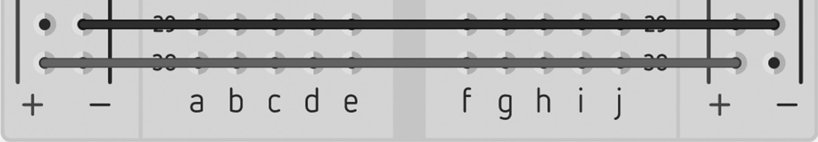
For the second project, we will build a parallel circuit powered by the Arduino based on the schematic in Figure 3.17.

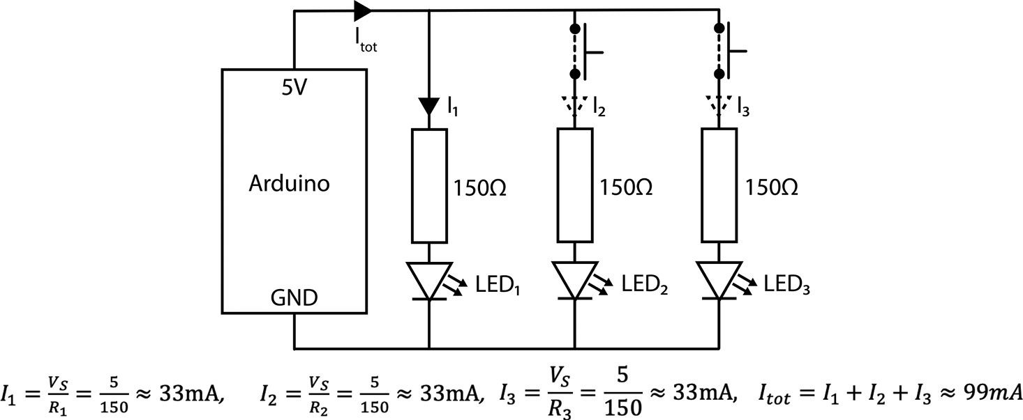
Figure 3.17Parallel circuit schematic. The schematic shows three branches connected in parallel with an Arduino power source, where the second and third branches are controlled by push-button switches. In each branch, a resistor controls the current flowing through an LED. The branch currents I1 and I3 are indicated with dashed lines for closed switch positions.

We recall that voltage is constant in a parallel circuit, so if the resistances are all equal to 150Ω then each branch current will also be equal (approximately 33mA $33 mA$ ). If the currents flowing through each branch are equivalent, then all three LEDs should light up with the same brightness. The previous project covered a lot of the practicalities of switch/resistor/LED component combinations, so we will move onto circuit design to see how we can use the breadboard to lay out our components in the most effective way possible.

Circuit design

In some respects, the circuit involved in this project will be a lot simpler to design and construct than the previous example. Other than the omission of the push-button switch from the first branch, each parallel branch of the circuit is the same so we can focus on designing a single section and then replicating it (Figure 3.18).

Figure 3.18First parallel circuit branch. This branch of the circuit is replicated throughout with the addition of push-button switches to create the full parallel circuit. The resistor LED combination should be familiar to you from the previous series circuit project design.

In the layout in Figure 3.18, the connections to the power rails are included to show another practicality of circuit design – you must always lay out each section of a circuit in relation to the signal or power pins that it will connect to. This becomes more apparent when we add one of the branches that also contains a push-button switch – the power rail must now be connected to the input of that switch before connecting it to the resistor/LED path (Figure 3.19).

Figure 3.19Second parallel circuit branch. In this branch of the circuit, a push-button switch has been added to control the flow of current. The first and second branches are shown together in the layout to illustrate how the resistor/LED combination in the first branch has been replicated.

Now we can simply replicate this branch to create the third branch of our circuit (Figure 3.20).

Figure 3.20Combined parallel circuit branches. This diagram shows the combined layout for all three parallel branches in the project circuit. The right-hand image shows the current flow for the entire circuit, where each parallel branch is connected to the common 5V and GND rails powered by the Arduino.

At this point, we can add power connections to Arduino. We will bridge the power rails (as in the previous circuit) to allow for our layout to be easily followed, though as noted at the beginning of this project we will ideally be aiming to reduce signal and power paths whenever possible (Figure 3.21).

Figure 3.21Final parallel circuit layout. All three branches of the circuit are shown connected to an Arduino for simulation in Tinkercad. This layout combines bottom-up and top-down components to maximize the space available on a single breadboard.

The final circuit layout for this project is now completed and ready for simulation testing in Tinkercad. Once this testing is complete, we can work through the specific pins needed to build the actual circuit in the steps below.

Project steps

For this project, you will need: 1. Arduino Uno board 2. One small breadboard (30 rows) 3. 3 × red LEDs 4. 3 × 150Ω resistors 5. 2 × push-button switches 6. 4 × connector cables and 6 × connector wires
Branch 1: 1. Add a 150Ω resistor between pins [i2–i5] 2. Add an LED – anode pin (h5) to cathode (h6) 3. Add a positive connector wire from [j1–V+] 4. Add a negative connector wire from [j6–GND]
To test the circuit, add a connector cable between the GND pin and the − power rail and a connector cable between the Arduino +5V pin and the + power rail. If it works: the LED should light up. Disconnect the Arduino power connector cable and continue to the next build stage. If it doesn’t work: check the placement of the resistor, check the push-button switch orientation and check the direction of the LED (long-leg cathode is positive).
Branch 2: 1. Add a push-button switch between pins [i8–g10] 2. Add a 150Ω resistor between pins [j10–j14] 3. Add an LED – anode pin (i14) to cathode (i15) 4. Add a positive connector wire from [j8–V+] 5. Add a negative connector wire from [j15–GND]
Reconnect the Arduino +5V pin to the + power rail and test the circuit by pushing the button. If it works: the second LED should light up with the first. Disconnect the Arduino power connector cable and continue to the next build stage. If it doesn’t work: check the placement of the branch 2 resistor, check the push-button switch orientation and check each LED’s direction.
Branch 3: 1. Add a push-button switch between pins [i17–g19] 2. Add a 150Ω resistor between pins [j19–j23] 3. Add an LED – anode pin (i23) to cathode (i24) 4. Add a positive connector wire from [j17–V+] 5. Add a negative connector wire from [j24–GND]
Reconnect the Arduino +5V pin to the + power rail and test the circuit by pushing each button in turn. If it works: the third LED should light up with the first. Disconnect the Arduino. If it doesn’t work: check the placement of the branch 3 resistor, check the push-button switch orientation and check each LED’s direction.

This circuit shows how parallel LEDs will have the same brightness because each branch current is equivalent. We know this because both the voltage (constant in a parallel circuit) and resistance are equal in each branch. At this point, we have now worked through the practical steps needed to build both series and parallel circuits, but there is now one last point to note about our circuits. In the first project, we connected three series loops to the same supply rails – this is also what we have done in the parallel circuit project. Thus, both circuits are effectively connected in parallel, which makes more sense if we now redraw the entire circuit from project 1 including the common Arduino power supply (Figure 3.22),

Figure 3.22Full project 1 schematic. *This diagram shows how the three series stages of the first project are effectively parallel branches within the overall Arduino circuit. The resistor and LED labels are omitted for clarity.*

This may initially seem slightly confusing, but the practical point is that we can design different circuit stages and power them from a common supply (the Arduino). For your own learning, the important point is not whether you see the first project circuit as series or parallel but rather that you understand how and why the circuit was divided into different stages. This is a very common circuit design task and you will see it again in later circuits in this book.

3.7 Conclusions

This chapter has covered a lot of ground, introducing Ohm’s Law, Kirchoff’s Laws (KVL, KCL) and also working through more involved project circuits. It is recommended that you spend some time going back through this chapter to make sure you are comfortable with the calculations involved – as noted in chapter 1, the mathematics may be fairly straightforward but working with symbols and scales can introduce a lot of pitfalls when you are beginning to learn electronics. If you find yourself struggling with some of the material in the next few chapters, it is highly likely that the root of the problem lies somewhere within the concepts and calculations introduced in this chapter – they may appear fairly simple in isolation, but we have worked through most of the core concepts of fundamental DC circuit analysis in a very short time and it is to be expected that you will take a little longer to synthesize everything you have just learned.

The next chapter will look at configuring and programming the Arduino for input processing and output control. This represents a significant shift in focus from DC circuit analysis, so be prepared to find the combination of new concepts more difficult to work through than any of the individual parts in isolation. As noted in chapter 1:

Applying these basic mathematical concepts requires practice – similarly, learning introductory code is not complex, but can be very confusing!

3.8 Self-study questions

The following questions use Ohm’s Law in combination with KVL and KCL to analyse series and parallel circuits. As we learned in chapter 1, the scales and symbols can often be much more difficult than the equations so be patient and don’t miss out any steps in your working. In addition, working with fractions is possibly less familiar to you so don’t forget the reciprocal in parallel circuits!

..................Content has been hidden....................

You can't read the all page of ebook, please click here login for view all page.

Table of Contents for
Chapter 3 DC circuits

Chapter 3

DC circuits

3.1 Ohm’s Law and direct current

3.1.1 Worked example – calculating a resistor value

3.2 Kirchoff’s Voltage Law: series circuits

3.2.1 Worked examples – calculating series resistance

3.2.2 Worked example – calculating series resistor voltages

3.3 Voltage dividers

3.3.1 Worked examples – voltage dividers

3.4 Kirchoff’s Current Law: parallel circuits

3.4.1 Worked examples – calculating parallel resistance

3.4.2 Worked examples – calculating parallel current

3.5 Tutorial: limiting current to protect components

3.6 Example projects: series and parallel circuits

3.6.1 Series circuit project

3.6.2 Parallel circuit project

3.7 Conclusions

3.8 Self-study questions

Table of Contents for Chapter 3 DC circuits

Create new playlist

Sign In

Sign Up

Table of Contents for
Chapter 3 DC circuits